Minimax Bridgeness-Based Clustering for Hyperspectral Data

Abstract

Hyperspectral (HS) imaging has been used extensively in remote sensing applications like agriculture, forestry, geology and marine science. HS pixel classification is an important task to help identify different classes of materials within a scene, such as different types of crops on a farm. However, this task is significantly hindered by the fact that HS pixels typically form high-dimensional clusters of arbitrary sizes and shapes in the feature space spanned by all spectral channels. This is even more of a challenge when ground truth data is difficult to obtain and when there is no reliable prior information about these clusters (e.g., number, typical shape, intrinsic dimensionality). In this letter, we present a new graph-based clustering approach for hyperspectral data mining that does not require ground truth data nor parameter tuning. It is based on the minimax distance, a measure of similarity between vertices on a graph. Using the silhouette index, we demonstrate that the minimax distance is more suitable to identify clusters in raw hyperspectral data than two other graph-based similarity measures: mutual proximity and shared nearest neighbours. We then introduce the minimax bridgeness-based clustering approach, and we demonstrate that it can discover clusters of interest in hyperspectral data better than comparable approaches.

1. Introduction

Hyperspectral (HS) imaging combines spectroscopy and imaging to capture the reflectance (or radiance) of surfaces within a scene. It is used in remote sensing applications to determine nutrient deficiency in crops [1], for vegetation mapping [2] or to model phytoplankton dynamics in the ocean [3]. The data produced by HS sensors is, however, very large (spatially) and HS pixels typically form high-dimensional clusters of arbitrary sizes and shapes in the feature space spanned by the spectral channels, which significantly hinders HS data mining. In remote sensing applications, ground truth data is often used for validation and information recovery in what is referred to as the supervised framework. However, obtaining such data is costly and time-demanding. “Ground truthing” involves surveying and processing campaigns with trained personnel, high-end equipment and laboratory tests. Furthermore, preparing ground truth data can be error-prone [4]. Semi-supervised or unsupervised methods are then highly desirable as they require little to no training data. In this paper, we focus on unsupervised classification, also known as clustering. Our objective is that each extracted cluster of pixels corresponds to a meaningful class of material within the scene. Furthermore, we also aim for the method to be easy to use and interpret, with no need for user input.

One of the main challenges in HS data clustering is that traditional distance metrics, such as the Euclidean distance, are meaningless in high-dimensional spaces [5,6]. Dimensionality reduction techniques, such as Principal/Independent Component Analysis [7,8,9], manifold learning [10] or band selection [11], have been used to address this issue, but they are also subject to the aforementioned problems, i.e., the need for ground truth data and the parameter tuning. In particular, the choice of an appropriate number of dimensions remains an open problem. However, we leave dimensionality reduction aspects outside the scope of this paper, as we focus solely on the clustering technique. In terms of comparing high-dimensional vectors, graph-based measures of similarity such as the number of shared nearest neighbours [12] and mutual proximity [13] have been proven useful to alleviate the curse of dimensionality [14]. The minimax distance [15] is another type of such measure, defined as the longest edge on a path between two distinct nodes of a graph, minimised over the range of all possible paths between the nodes. It is also the longest edge on the path between two nodes of a minimum spanning tree. The minimax distance is very powerful to separate clusters of arbitrary shape, size and dimensionality, especially if the data is relatively noise-free [16,17]. Furthermore, unlike the shared nearest neighbours, the minimax distance is completely parameter-free. In this paper, we propose a clustering method that harnesses the advantages of the minimax distance for HS data mining. The method creates a minimum spanning tree and determines which edges are most likely bridges between clusters based on four intuitive and parameter-free heuristics that we introduce. It then works as a sequential graph partitioning approach using the silhouette index as an objective function. In the next sections, we review related work, present the minimax distance and demonstrate its suitability for the task. We then introduce the proposed clustering approach, present results and conclude.

2. Related Work

Unsupervised classification of HS data has been an active research topic for several decades with many existing methods based on template-matching, spectral decomposition, density analysis or hierarchical representation [18]. Recent trends have also seen the emergence of deep models [19,20] that can model the distribution of information in high-dimensional data. However, these methods currently do not generalise nor scale well and require a tremendous amount of training data. The main drawback with template-matching methods (e.g., centroid-based, mixture of Gaussians) is that the shape of the clusters is presumed known a priori, i.e., they are parametric. For example, K-means and its variants are primarily meant to detect convex-shaped clusters, which occur only rarely in HS data. In spectral clustering [21,22], the eigenvectors of a Laplacian matrix representing the data are used to project the clusters in a subspace where they are more separable. Performance depends on how the Laplacian is defined and how clustering is eventually performed after projecting the data.

Clustering based on density analysis has received a lot of attention in the geoscience and remote sensing communities. Their rationale is that pixels are sampled from a multivariate probability density function (PDF) of unknown shape and parameters, which can be estimated from the data. Most methods are based on a search for the local maxima of the PDF, also referred to as modes. Most existing mode-seeking approaches, such as Mean Shift [23,24] or Fast Density Peak Clustering [25], assume that each cluster contains a single dominant mode, although it may not always be true (consider for instance the case of a ring-shaped cluster). This motivates methods, such as those based on space partitioning [26], or support vector machines [27], that seek local minima of the density functions as they represent the boundaries between clusters. These methods are independent of cluster shape. DBSCAN (Density-based spatial clustering of applications with noise) [28] is another adaptive approach in which “core points” are selected to better separate clusters and facilitate their extraction. Unfortunately, the performance of DBSCAN and most density-based clustering methods depend heavily on parameter tuning, which generally comes down to finding the right amount of smoothing for density estimation. This problem also applies also to k nearest neighbours (kNN)-based methods [29,30,31] as k is generally not an intuitive parameter for end-users. Automatic tuning with the elbow method [32,33] gives no theoretical guarantee of finding the optimal parameter. Adaptive density estimation (e.g., based on diffusion [34]) requires a lot of data to find significant patterns in high dimensions, and there is currently no consensus on whether they can outperform global methods on high-dimensional data [35].

Parameter-laden algorithms present an important pitfall as incorrect settings may prevent the retrieval of the true patterns and instead lead the algorithm to greatly overestimate the significance of less relevant ones [36]. This makes parameter setting a burden to the end-user. Existing parameter-free approaches are based on finding either a natural cutoff or peaks in some distribution [37,38] or rely on maximising a quality criterion [39] or combining strategies [40]. The recently proposed FINCH [41] is based on a simple and intuitive nearest-neighbour rule and hierarchically combines clusters based on the position of their respective means.

To address the problem of similarity in high dimensions, an effective approach consists of comparing points in terms of their neighbourhoods rather than only their coordinates. The number of shared nearest neighbours [14,42] is based on this principle, but it requires setting k, the neighbourhood size. A parameter-free alternative known as mutual proximity [13], has also shown promise for clustering but, as we will demonstrate, it leads to sub-optimal performance, and it comes at a high computational cost. The minimax distance is another type of graph-based similarity measure that shows promise for data classification [15]. In this paper, our main contributions are an evaluation of graph-based similarity measures based on the silhouette coefficient, as well as a new parameter-free clustering algorithm named MBC (Minimax Bridgeness-based Clustering).

3. The Minimax Distance

3.1. Definition

Consider a connected, undirected and edge-weighted graph $\mathbf{G}(V,E)$ where $V=\left\{v_i\right|i=1..N\}$ is a set of N vertices and $E=\left\{e_i\right|i=1..M\}$ is a set of M edges, with $N<M$. Note $\mathbf{P}\left(v_i,v_j\right)$ the set of all loopless paths between vertices i and j in $\mathbf{G}$. The largest of all edge weights along a given path $p\left(v_i,v_j\right)$ is denoted $w_{\max }\left(p\right)$. Then, the path that satisfies:

$$p_{\mathrm{mnx}}\left(v_i,v_j\right)=\underset{p}{\mathrm{argmin}}\left[w_{\max }\left(p\right)\right],p\in \mathbf{P}\left(v_i,v_j\right)$$

(1)

is the minimax path between vertices i and j. The edge in which the weight is $w_{\max }\left(p_{\mathrm{mnx}}\left(v_i,v_j\right)\right)$ will be referred to as the minimax edge, its weight is the minimax distance between vertices i and j.

The minimax distance matrix, similarly to the mutual proximity and shared nearest neighbours distance matrices, is computed based on E, the weights of the graph. These weights typically represent the Euclidean distance. They can be obtained from the data in $\mathcal{O}\left(n^2\right)$, with n the number of data points, but parallel computing can be used to increase efficiency [43,44]. The minimax distance matrix is then computed based a minimum spanning tree (MST) on $\mathbf{G}$, which constitutes a subset of E. An MST is defined as a set of edges that connects all the data points, without any cycles and with the smallest total edge weight. Each edge of an MST is a minimax edge [15], and the distance matrix can then be obtained in linear time from the MST [45], which can also be constructed in linear time [46].

3.2. Minimax Silhouette

An ideal measure of similarity should be so that it returns a small value if the data points belong to the same class and a large value otherwise. This property is captured by the silhouette index, which measures how similar a data point x is to its own cluster compared to other clusters:

$$s\left(x\right)=\frac{b\left(x\right)-a\left(x\right)}{max\left\{a\left(x\right),b\left(x\right)\right\}}$$

(2)

where $s\left(x\right)$ is the silhouette of x, $a\left(x\right)$ is the average similarity between x and all other points in the same cluster and $b\left(x\right)$ is the smallest average similarity x and all other points in different clusters. A small average silhouette indicates that clusters are poorly separated, and negative values mean that they overlap significantly. While the silhouette index is typically used to assess a clustering result, we use it here to compare similarity measures. We calculated the average silhouette of the ground truth of each of the data-sets described in Section 5.2, with the squared Euclidean norm, the spectral angle mapper and their respective minimax, mutual proximity and shared nearest neighbours versions.

In

Table 1. Comparison of similarity measures in terms of average ground truth silhouette (higher is better). SE: Squared Euclidean norm, SAM: Spectral Angle Mapper.

		Pavia U.	KSC	Salinas	Botswana	Massey
Regular	SE	−0.744	−0.693	−0.461	−0.604	−0.742
	SAM	−0.742	−0.500	−0.428	−0.616	−0.686
SNN	SE	−0.160	−0.245	−0.214	−0.216	−0.094
	SAM	−0.087	−0.209	−0.189	−0.236	−0.184
Mutual Proximity	SE	−0.123	−0.207	−0.035	−0.028	−0.182
	SAM	−0.156	−0.071	−0.087	−0.084	−0.075
Minimax	SE	−0.047	−0.019	0.021	0.015	−0.256
	SAM	−0.123	−0.256	−0.021	−0.104	−0.261
Mutual Proximity on ${\Gamma }_{50}$	SE	−0.038	−0.108	0.038	0.037	−0.115
	SAM	−0.164	−0.042	0.062	−0.194	0.026
Minimax on ${\Gamma }_{50}$	SE	0.128	0.260	0.212	0.174	−0.115
	SAM	0.196	−0.087	0.194	−0.046	−0.349

, we report the results obtained on the whole data-set (limited to 10,000 points—see Section 5.2) or only on a core set ${\Gamma }_{50}$ consisting of the 50% data points of highest density (see next paragraph). We then compared the regular measures, i.e., Squared Euclidean norm (SE) and Spectral Angle Mapper (SAM), to their corresponding shared nearest neighbour (SNN), mutual proximity and minimax distance counterparts. Note that SNN requires to tune the parameter k, i.e., the size of the set of NN within which the shared neighbours are searched for each pair of pixels. The results we report are the best from all values of k between 5 and N, with a step size of 5. These results indicate that even the largest silhouette (0.260 with Minimax SE on ${\Gamma }_{50}$) is relatively low, confirming that HS clusters are generally not well separable in the feature space spanned by all spectral bands. Nevertheless, we can observe the clear inferiority of the regular measures, with a full-set silhouette of −0.428 at most. The minimax distance and mutual proximity surpass the shared nearest neighbours overall, except on the Massey data. Further, note the improvement obtained by discarding the 50% least dense (i.e., noisiest) pixels, particularly for the minimax distance, which gives the best results overall. This suggests that the minimax distance is better suited to extract classes of interest from HS data, especially on core sets.

Using the core set ${\Gamma }_{50}$ allows to tackle two drawbacks of the minimax distance: sensitivity to noise and computational complexity. Core sets have previously been used for similar purposes [28,40,47]. To select a representative core set in a computationally efficient and parameter-free manner, we estimate the underlying probability density function of the data and discard the 50% least dense points. We compared several parameter-free and scalable density estimators in terms of their ability to produce core sets with compact and well-separated classes at several threshold values [48]. It is particularly noteworthy that diffusion-based approaches [34] scale poorly to high-dimensional data and suffer from the Hughes phenomenon: they require a tremendous amount of sampling points to correctly estimate the multivariate density. Instead, we found that convolving the data with an isotropic Gaussian kernel with a bandwidth equal to the average distance to a point’s nearest neighbour allowed for a good balance between low computational footprint and usefulness in identifying core-sets. We used this approach to estimate density in the remainder of our experiments.

3.3. Minimax Distance-Based kNN Clustering

In order to further demonstrate the usefulness of the minimax distance, we compared the performance of two state-of-the-art kNN-based algorithms: KNNCLUST [49] and GWENN [50]. Both rely on a measure of distance to perform clustering. We evaluated whether using the minimax distance can improve performance in terms of overall accuracy (OA) and cluster purity [51] on the five data-sets presented in Section 5.2. Figure 1 shows results obtained on one of these data-sets. Note that, for a given data point x in the feature space, all its neighbours that are at the same minimax distance to x are sorted based on regular distance.

Results indicate that using the minimax distance can improve the performance of kNN-based clustering on HS data. On all five data-sets, the peak overall accuracy was improved by at least 3% and up to 8% (on the Kennedy Space Centre scene), and cluster purity was improved for most values of k. We also found that, as k increases, the number of clusters decreases. This should be considered when evaluating cluster purity, which is known to increase with the number of clusters. Purity is a more meaningful measure of clustering quality when this number is low, which is the case in our experiments.

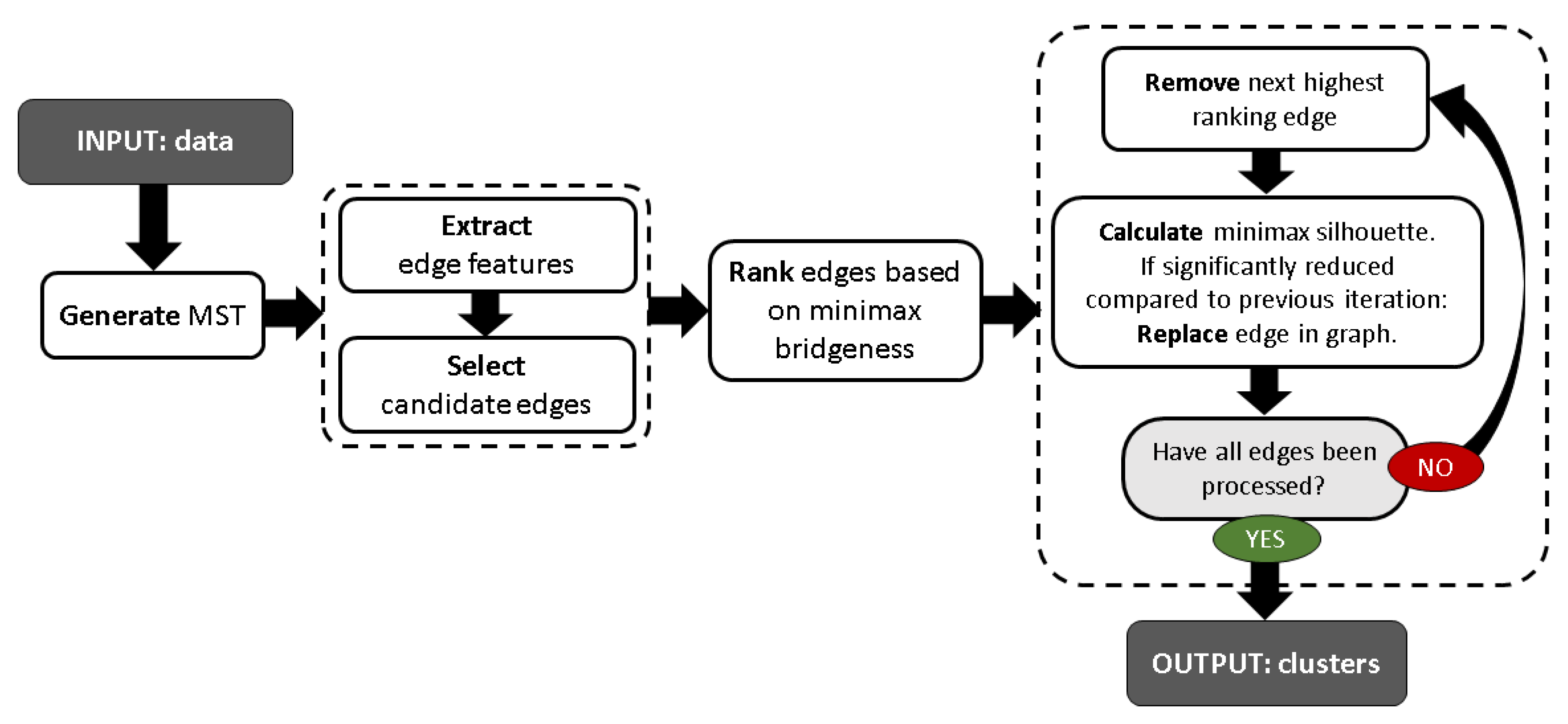
4. Minimax Bridgeness-Based Clustering

As we demonstrated, the minimax distance is well suited for class separation in HS data. However, a large minimax distance informs only of the existence of a gap on a path between two points, but not so much of its significance. The latter can be established when the gap’s existence is confirmed by multiple pairs of end-nodes. The number of these pairs gives what we refer to as the minimax bridgeness: $\beta \left(E\right)$, where E is an edge in $\mathbf{G}$. It can also be defined as the number of paths on which E is a minimax edge. A high bridgeness indicates a consensus between data points that the node crosses a border between clusters. Figure 2 illustrates the concept of minimax bridgeness with a simple example.

The proposed clustering algorithm, hereby referred to as Minimax Bridgeness-based Clustering (MBC), works as a sequential graph partitioning with four main steps (see Figure 3):

• Step 1: Compute minimum spanning tree (MST).
• Step 2: Discard edges that are unlikely to separate clusters.
• Step 3: Rank the remaining edges based on minimax bridgeness.
• Step 4: Remove next highest ranking edge that does not significantly decrease the minimax silhouette. Repeat until all edges have been assessed.

For Step 1, there are numerous algorithms to extract the MST of the data efficiently, but we consider these aspects outside the scope of this paper. Note that the MST is unique if all pairwise distances between pixels are different.

In Step 2, to find edges that are unlikely to be inter-cluster bridges (ICBs), we first identify four important properties of ICBs:

• They are longer than most edges.
• They have a higher minimax bridgeness than most edges.
• They have a lower density point at their centre than most edges.
• Neither of the vertices they connect is the other’s first neighbour, nor do they have the same nearest neighbour (see [41]).

With regards to the first three properties listed above, we found that the distributions of edge length, minimax bridgeness and central point density typically have a single dominant mode each. Specifically, we use diffusion-based density estimation [34] to determine the peak locations and estimate these modes. We observed that, for at least one of these three attributes, ICBs always have a value significantly larger than the mode. We then established that edges that do not satisfy this property are unlikely to be ICBs. Note that we tested various density estimation methods, keeping in mind that we need a parameter-free and computationally efficient method to increase clustering performance, first by allowing for better identification of ICBs, and then by creating a representative subset $\Gamma$ of the data. The latter can be used to create a pseudo-ground truth of the data and apply a more computationally-efficient clustering on the remaining data points. As previously mentioned, we found that an isotropic Gaussian kernel with a bandwidth equal to the average distance to any point’s nearest neighbour gave the best results overall.

Finally, in Steps 3 and 4, we use the minimax silhouette as guiding criterion. In an approach similar to that employed in GWENN [50], candidate edges are ranked in order of descending $\beta$ and removed one by one in a sequential manner. The edge with the largest $\beta$ is systematically removed. The minimax silhouette then is calculated after each edge removal. If the edge removed last caused the silhouette to decrease by more than half its value at the previous iteration, or to become negative, the edge is put back in the graph. This ad hoc rule is particularly efficient when the data contains well-separated clusters. As previously demonstrated, the minimax silhouette captures cluster separation better than other measures of distances on HS data. Our experiments showed that removing an edge that does not separate clusters tend to decrease the minimax silhouette by more than half its current value.

5. Experimental Validation

5.1. Alternative Clustering Methods

To validate the proposed method, we compared it to five state-of-the-art clustering methods, which are summarised in

Table 2. Characteristics of the clustering methods used for comparison to this study.

	Parameters	Pros	Cons
FCM [52]	K, m	fuzzy	fitted to convex clusters
FDPC [25]	$d_c$	fast	requires decision graph
DBSCAN [28]	$d_{min}$, $Eps$	fast	not scalable
GWENN [50]	k	non iterative	requires NN search
FINCH [41]	-	parameter-free	requires NN search
Laplacian centrality-based (LPC) [38]	-	parameter-free	not scalable

.

Note that the latter two are parameter-free. Fuzzy C-means requires the number of clusters K and a (typically parametrised) de-fuzzification parameter m. For FDPC and GWENN, we manually tuned their respective parameter to obtain the right number of clusters. We also implemented a variant of MBC, which allows specifying the number of clusters K. We named it K-MBC. In this case, the iterative approach of step 4 stops when $K-1$ edges have been removed or when all edges not discarded in step 2 have been examined, whichever comes first. Finally, we evaluated MBC on ${\Gamma }_{50}$ for each data-set to determine how it performs on a smaller and cleaner set of points.

5.2. Data

We used five HS images: Pavia University, Kennedy Space Centre, Salinas, Botswana and Massey University.

The Pavia University image was acquired over Pavia, Italy (Lat-Long coordinates of scene centre: 45°12′06″N, 9°08′08″E), by the airborne ROSIS (Reflective Optics System Imaging Spectrometer) sensor operated by the German Aerospace Agency (DLR). It contains $610\times 340$ pixels (ground resolution: 1.3 m) and 103 spectral bands (430 to 860 nm). Nine classes (Asphalt, Meadows, Gravel, Trees, Painted metal sheets, Bare soil, Bitumen, Self-blocking bricks, Shadow) are provided as ground truth.

The KSC image was acquired over the Kennedy Space Centre, Florida (Lat-Long coordinates of scene centre: 28°37′50″N, 80°46′45″W), by the airborne AVIRIS (Airborne Visible/Infrared Imaging Spectrometer) NASA instrument. It contains 224 spectral bands (400 to 2500 nm), but only 176 of them were kept after water absorption bands removal. The ground resolution is 18 m and the ground truth is made of 13 classes (Scrub, Willow swamp, CP hammock, CP/Oak, Slash pine, Oak/Broadleaf, Hardwood swamp, Graminoid marsh, Spartina marsh, Cattail marsh, Salt marsh, Mud flats, Water).

The Salinas HSI was also acquired by AVIRIS sensor over agricultural fields in the Salinas Valley, California (Lat-Long coordinates of scene centre: 36°18′39″N, 121°13′15″W). It has $512\times 217$ pixels (ground resolution: 3.7 m). Twenty absorption bands were removed from the 224 original bands. The ground truth comprises 16 vegetation classes (Broccoli gr. wds 1, Broccoli gr. wds, Fallow, Fallow rough plow, Fallow smooth, Stubble, Celery, Grapes untrained, Soil vineyard develop, Corn sen. gr. wds, Lettuce romaine 4 wk, Lettuce romaine 5 wk, Lettuce romaine 6 wk, Lettuce romaine 7 wk, Vineyard untrained, Vineyard vert. trellis).

The Botswana HSI was acquired over the Okavango Delta, Botswana (Lat-Long coordinates of scene centre: 19°33′33″S, 23°07′37″E), by the Hyperion sensor onboard the EO-1 satellite (within the same spectral range than AVIRIS), with a ground resolution of 30 m. It has $1476\times 256$ pixels and 145 bands (from 242 original bands) after water absorption bands removal. The ground truth map includes 14 classes (Water, Hippo grass, Floodplain Grasses 1, Floodplain Grasses 2, Reeds, Riparian, Firescar 2, Island interior, Acacia woodlands, Acacia shrublands, Acacia grasslands, Short mopane, Mixed mopane, Exposed soils).

The Massey University scene [53] was captured in Palmerston North, New Zealand (Lat-Long coordinates of scene centre: 40°23′17″S, 175°37′07″E), with an airborne AisaFENIX hyperspectral sensor covering visible to short-wave infrared (380 to 2500 nm). It has 339 bands (after removal of water absorption and noisy bands) and 9564 pixels with corresponding ground truth. The latter contains a total of 23 different land-cover classes, which includes nine different types of roof tops, five vegetation types, water, soil, and two different shadows.

The characteristics of these five data sets are summarised in

Table 3. Description of data-sets used: number of labelled pixels N, dimensionality D and number of classes.

Data-Set	N	D	Classes
Pavia University	42,776	103	9
Kennedy Space Centre	5211	176	13
Salinas	54,129	204	16
Botswana	3248	145	14
Massey University	9564	339	23

and their colour composite are shown in Figure 4.

The data was pre-processed to remove noisy spectral bands, burnt pixels and inconsistent ground truth data (see [4]). Furthermore, the number of pixels was capped to 10,000 per scene, mostly due to the memory complexity incurred by the computation of the similarity matrix. For each data-set with more than 10,000 pixels, we performed 20 random selections (Note that the same proportion of each class was kept after subsampling.) of 10,000 points and computed the average results.

5.3. Criteria

The criteria used to validate the proposed approach and compare it to other state-of-the-art methods are as follows:

• Overall Accuracy (OA) (see

  Table 4. Comparison of clustering results: Overall Accuracy (%).

  Number of Clusters Is		Pavia U.	KSC	Salinas	Botswana	Massey U.
  Known	FCM	41.9	52.5	54.6	61.4	43.3
  	FDPC	44.2	47.6	62.2	62.4	54.0
  	GWENN	47.9	49.8	65.3	53.5	44.3
  	K-MBC	65.9	58.2	76.5	51.2	70.0
  Unknown	FINCH	37.0	39.7	55.7	56.2	38.6
  	LPC	35.2	42.4	59.2	54.2	41.6
  	MBC	64.2	51.2	76.2	42.3	53.3
  	MBC on ${\Gamma }_{50}$	70.1	59.1	80.0	60.5	65.7

  ) is the average number of pixels that are correctly classified. It is calculated as the sum of diagonal elements of the confusion matrix divided by the total number of pixels. Here, the confusion matrix is obtained owing to the Hungarian (Munkres) algorithm [54].
• Purity [51] (see

  Table 5. Comparison of clustering results: Purity (higher is better, max: 1).

  Number of Clusters Is		Pavia U.	KSC	Salinas	Botswana	Massey U.
  Known	FCM	0.47	0.56	0.63	0.65	0.47
  	FDPC	0.54	0.64	0.71	0.81	0.59
  	GWENN	0.62	0.69	0.77	0.73	0.82
  	K-MBC	0.91	0.74	0.93	0.97	0.74
  Unknown	FINCH	0.42	0.42	0.59	0.58	0.42
  	LPC	0.39	0.44	0.59	0.59	0.60
  	MBC	0.97	0.70	0.91	0.96	0.60
  	MBC on ${\Gamma }_{50}$	0.96	0.73	0.95	0.97	0.80

  ) measures the tendency of clusters to contain a single class.
• Normalised Mutual Information (NMI) (see

  Table 6. Comparison of clustering results: Normalised Mutual Information (NMI) (higher is better, max: 1).

  Number of Clusters Is		Pavia U.	KSC	Salinas	Botswana	Massey U.
  Known	FCM	0.49	0.58	0.69	0.68	0.60
  	FDPC	0.49	0.59	0.74	0.74	0.69
  	GWENN	0.48	0.60	0.72	0.61	0.57
  	K-MBC	0.62	0.71	0.85	0.47	0.76
  Unknown	FINCH	0.49	0.60	0.75	0.72	0.69
  	LPC	0.49	0.57	0.72	0.69	0.53
  	MBC	0.62	0.62	0.84	0.44	0.77
  	MBC on ${\Gamma }_{50}$	0.63	0.70	0.87	0.61	0.79

  ) measures the probabilistic resemblance between cluster and class labels.
• The average difference between the number of classes and the number of clusters (see

  Table 7. Comparison of clustering results: Average difference between number of classes and number of discovered clusters. Negative values mean that too many clusters were discovered by the method.

  	Pavia U.	KSC	Salinas	Botswana	Massey U.
  FINCH	−13	−20	−17	−12	−15
  LPC	−14	−20	−16	−14	−17
  MBC	3	2	1	6	−4
  MBC on ${\Gamma }_{50}$	0	2	0	4	−1

  ).

In terms of computational cost, we found that it takes about 2 min to cluster 10,000 points with MBC with a Matlab implementation (hardware: x64-based Intel Core i7-8750H CPU @ 2.20GHz, 32GB of RAM), mostly spent on the creation of graph $\mathbf{G}$ from the data.

5.4. Results

From these results, we make the following observations:

• K-MBC significantly outperforms FCM, FDPC and GWENN on all data-sets except Botswana in terms of OA and NMI. It also yields the best pixel purity on all data-sets except Massey University, where it is surpassed only by GWENN by 0.08.
• The clustering maps in Figure 5 confirm that our approach performs particularly well at creating clusters of high purity.
• Although it is expected that MBC would give the best overall results when applied to the core set ${\Gamma }_{50}$, or when the number of clusters is known, this does not appear as obvious from our results. However, we note that MBC tends to find too few clusters in the data (especially on the Botswana data-set, where it misses six classes of pixels).
• FINCH and LPC generally perform poorly overall and especially in terms of number of clusters. They each tend to detect too many clusters on all data-sets. Interestingly, they also yield poor pixel purity values. Usually, high purity is expected when the number of clusters is high. The fact that we observe the contrary indicates that these two methods are really not well suited to deal with raw hyperspectral data.
• On the core-set ${\Gamma }_{50}$, MBC performs very well and even finds the right number of clusters in the Pavia University and Salinas scenes. It over-estimates this number by one on the Massey University scene and under-estimate by two on the KSC scene.
• The Botswana scene seems to the most challenging for the proposed methods. The only case where the MBC clustering surpasses the benchmark with this scene is in terms of pixel purity. We noted that this particular scene contains classes of pixels that are among the least pure in the benchmark, with strong variations in reflectance spectra within classes. We hypothesise that this is the main reason for our method under-performing on this scene. On the other hand, it is well known that clustering is generally an ill-posed problem and that different applications may require different types of clustering approaches. Clearly, in this case, FDPC performs better, but it should be noted that it was tuned manually, unlike MBC.

Overall, these results indicate that MBC can handle high-dimensional data well and recognise meaningful classes of materials and surfaces in a scene. While it comes with a certain computational cost, it performs better than existing clustering methods, even without parameter tuning. These results also validate our hypothesis that the minimax distance is well suited for hyperspectral data exploration.

6. Conclusions

We introduced MBC, a parameter-free clustering algorithm based on a new graph-based measure of similarity, which we named minimax bridgeness. We demonstrated its ability to automatically discover clusters in high-dimensional remote sensing data without user input, as well as its superiority over other graph-based similarity measures such as the number of shared nearest neighbours. The proposed method has two drawbacks: its sensitivity to noise and its high computational cost. To address these, we used a simple approach based on density estimation to select a subset of relevant data points, a so-called core set and applied MBC on it, which resulted in stronger performance across the board. Future work should focus on the selection of core sets for a more efficient exploitation of the minimax distance and minimax bridgeness. Also, the use of unsupervised dimensionality reduction techniques based, for instance, on band selection is expected to improve performance by reducing the curse of dimensionality. Lastly, future work should also focus on developing efficient methods to produce graph-based similarity matrices that scale to large data-sets.

References

1. Cilia, C.; Panigada, C.; Rossini, M.; Meroni, M.; Busetto, L.; Amaducci, S.; Boschetti, M.; Picchi, V.; Colombo, R. Nitrogen status assessment for variable rate fertilization in maize through hyperspectral imagery. Remote Sens. 2014, 6, 6549–6565. [Google Scholar] [CrossRef] [Green Version]
2. Adão, T.; Hruška, J.; Pádua, L.; Bessa, J.; Peres, E.; Morais, R.; Sousa, J. Hyperspectral imaging: A review on UAV-based sensors, data processing and applications for agriculture and forestry. Remote Sens. 2017, 9, 1110. [Google Scholar] [CrossRef] [Green Version]
3. Groom, S.B.; Sathyendranath, S.; Ban, Y.; Bernard, S.; Brewin, B.; Brotas, V.; Brockmann, C.; Chauhan, P.; Choi, J.K.; Chuprin, A.; et al. Satellite ocean colour: Current status and future perspective. Front. Mar. Sci. 2019, 6, 485. [Google Scholar] [CrossRef] [Green Version]
4. Chehdi, K.; Cariou, C. Learning or assessment of classification algorithms relying on biased ground truth data: What interest? J. Appl. Remote Sens. 2019, 13, 1–26. [Google Scholar] [CrossRef]
5. Aggarwal, C.C.; Hinneburg, A.; Keim, D.A. On the Surprising Behavior of Distance Metrics in High Dimensional Space; Lecture Notes in Computer Science; Springer: Berlin/Heidelberg, Germany, 2001; Volume 1973, pp. 420–434. [Google Scholar]
6. Murphy, J.M.; Maggioni, M. Unsupervised Clustering and Active Learning of Hyperspectral Images With Nonlinear Diffusion. IEEE Trans. Geosci. Remote Sens. 2018, 57, 1829–1845. [Google Scholar] [CrossRef] [Green Version]
7. Wang, J.; Chang, C. Independent component analysis-based dimensionality reduction with applications in hyperspectral image analysis. IEEE Trans. Geosci. Remote Sens. 2006, 44, 1586–1600. [Google Scholar] [CrossRef]
8. Fauvel, M.; Chanussot, J.; Benediktsson, J. Kernel principal component analysis for feature reduction in hyperspectrale images analysis. In Proceedings of the 7th Nordic Signal Processing Symposium—NORSIG 2006, Rejkjavik, Iceland, 7–9 June 2006; IEEE: Piscataway, NJ, USA, 2006; pp. 238–241. [Google Scholar]
9. Pandey, P.C.; Tate, N.J.; Balzter, H. Mapping tree species in coastal portugal using statistically segmented principal component analysis and other methods. IEEE Sens. J. 2014, 14, 4434–4441. [Google Scholar] [CrossRef] [Green Version]
10. Bachmann, C.M.; Ainsworth, T.L.; Fusina, R.A. Exploiting manifold geometry in hyperspectral imagery. IEEE Trans. Geosci. Remote Sens. 2005, 43, 441–454. [Google Scholar] [CrossRef]
11. Chang, C.; Wang, S. Constrained band selection for hyperspectral imagery. IEEE Trans. Geosci. Remote Sens. 2006, 44, 1575–1585. [Google Scholar] [CrossRef]
12. Jarvis, R.A.; Patrick, E.A. Clustering using a similarity measure based on shared near neighbors. IEEE Trans. Comput. 1973, 100, 1025–1034. [Google Scholar] [CrossRef]
13. Schnitzer, D.; Flexer, A.; Schedl, M.; Widmer, G. Local and global scaling reduce hubs in space. J. Mach. Learn. Res. 2012, 13, 2871–2902. [Google Scholar]
14. Stevens, J.R.; Resmini, R.G.; Messinger, D.W. Spectral-Density-Based Graph Construction Techniques for Hyperspectral Image Analysis. IEEE Trans. Geosci. Remote Sens. 2017, 55, 5966–5983. [Google Scholar] [CrossRef]
15. Chehreghani, M.H. Classification with Minimax Distance Measures. In Proceedings of the Thirty-First AAAI Conference on Artificial Intelligence, San Francisco, CA, USA, 4–10 February 2017; pp. 1784–1790. [Google Scholar]
16. Grygorash, O.; Zhou, Y.; Jorgensen, Z. Minimum spanning tree based clustering algorithms. In Proceedings of the 18th IEEE International Conference on Tools with Artificial Intelligence, ICTAI’06, Arlington, VA, USA, 13–15 November 2006; IEEE: Piscataway, NJ, USA, 2006; pp. 73–81. [Google Scholar]
17. Little, A.; Maggioni, M.; Murphy, J.M. Path-based spectral clustering: Guarantees, robustness to outliers, and fast algorithms. arXiv 2017, arXiv:1712.06206. [Google Scholar]
18. Saxena, A.; Prasad, M.; Gupta, A.; Bharill, N.; Patel, O.P.; Tiwari, A.; Er, M.J.; Ding, W.; Lin, C.T. A review of clustering techniques and developments. Neurocomputing 2017, 267, 664–681. [Google Scholar] [CrossRef] [Green Version]
19. Xie, J.; Girshick, R.; Farhadi, A. Unsupervised deep embedding for clustering analysis. In Proceedings of the International Conference on Machine Learning, New York, NY, USA, 19–24 June 2016; pp. 478–487. [Google Scholar]
20. Yang, J.; Parikh, D.; Batra, D. Joint unsupervised learning of deep representations and image clusters. In Proceedings of the IEEE Conference on Computer Vision and Pattern Recognition, Las Vegas, NV, USA, 26 June–1 July 2016; pp. 5147–5156. [Google Scholar]
21. Ng, A.Y.; Jordan, M.I.; Weiss, Y. On spectral clustering: Analysis and an algorithm. In Advances in Neural Information Processing Systems; MIT Press: Cambridge, MA, USA, 2002; pp. 849–856. [Google Scholar]
22. Wang, X.F.; Xu, Y. Fast clustering using adaptive density peak detection. Stat. Methods Med. Res. 2017, 26, 2800–2811. [Google Scholar] [CrossRef] [PubMed]
23. Fukunaga, K.; Hostetler, L.D. The estimation of the gradient of a density function, with applications in pattern recognition. IEEE Trans. Inf. Theory 1975, 21, 32–40. [Google Scholar] [CrossRef] [Green Version]
24. Comaniciu, D.; Meer, P. Mean Shift: A Robust Approach Toward Feature Space Analysis. IEEE Trans. Pattern Anal. Mach. Intell. 2002, 24, 603–619. [Google Scholar] [CrossRef] [Green Version]
25. Rodriguez, A.; Laio, A. Clustering by fast search and find of density peaks. Science 2014, 344, 1492–1496. [Google Scholar] [CrossRef] [Green Version]
26. Lu, L.; Jiang, H.; Wong, W.H. Multivariate density estimation by bayesian sequential partitioning. J. Am. Stat. Assoc. 2013, 108, 1402–1410. [Google Scholar] [CrossRef]
27. Mantero, P.; Moser, G.; Serpico, S.B. Partially supervised classification of remote sensing images through SVM-based probability density estimation. IEEE Trans. Geosci. Remote Sens. 2005, 43, 559–570. [Google Scholar] [CrossRef]
28. Ester, M.; Kriegel, H.P.; Sander, J.; Xu, X. A density-based algorithm for discovering clusters in large spatial databases with noise. Kdd 1996, 96, 226–231. [Google Scholar]
29. Loftsgaarden, D.O.; Quesenberry, C.P. A nonparametric estimate of a multivariate density function. Ann. Math. Stat. 1965, 36, 1049–1051. [Google Scholar] [CrossRef]
30. Cariou, C.; Chehdi, K. Nearest neighbor-density-based clustering methods for large hyperspectral images. In Image and Signal Processing for Remote Sensing XXIII; International Society for Optics and Photonics: Bellingham WA, USA, 2017; Volume 10427, p. 104270I. [Google Scholar]
31. Geng, Y.A.; Li, Q.; Zheng, R.; Zhuang, F.; He, R.; Xiong, N. RECOME: A new density-based clustering algorithm using relative KNN kernel density. Inf. Sci. 2018, 436, 13–30. [Google Scholar] [CrossRef] [Green Version]
32. Thorndike, R.L. Who belongs in the family. In Psychometrika; Citeseer: Princeton, NJ, USA, 1953. [Google Scholar]
33. Goutte, C.; Toft, P.; Rostrup, E.; Nielsen, F.A.; Hansen, L.K. On clustering fMRI time series. NeuroImage 1999, 9, 298–310. [Google Scholar] [CrossRef] [Green Version]
34. Botev, Z.I.; Grotowski, J.F.; Kroese, D.P. Kernel density estimation via diffusion. Ann. Stat. 2010, 38, 2916–2957. [Google Scholar] [CrossRef] [Green Version]
35. Ketchen, D.J.; Shook, C.L. The application of cluster analysis in strategic management research: An analysis and critique. Strateg. Manag. J. 1996, 17, 441–458. [Google Scholar] [CrossRef]
36. Keogh, E.; Lonardi, S.; Ratanamahatana, C.A. Towards parameter-free data mining. In Proceedings of the Tenth ACM SIGKDD International Conference on Knowledge Discovery and Data Mining, Seattle, WA, USA, 22–25 August 2004; ACM: New York, NY, USA, 2004; pp. 206–215. [Google Scholar]
37. Koonsanit, K.; Jaruskulchai, C.; Eiumnoh, A. Parameter-free K-means clustering algorithm for satellite imagery application. In Proceedings of the International Conf. on Information Science and Applications, Suwon, Korea, 23–25 May 2012; IEEE: Piscataway, NJ, USA, 2012; pp. 1–6. [Google Scholar]
38. Yang, X.H.; Zhu, Q.P.; Huang, Y.J.; Xiao, J.; Wang, L.; Tong, F.C. Parameter-free Laplacian centrality peaks clustering. Pattern Recognit. Lett. 2017, 100, 167–173. [Google Scholar] [CrossRef]
39. Cesario, E.; Manco, G.; Ortale, R. Top-down parameter-free clustering of high-dimensional categorical data. IEEE Trans. Knowl. Data Eng. 2007, 19, 1607–1624. [Google Scholar] [CrossRef]
40. Hou, J.; Gao, H.; Li, X. DSets-DBSCAN: A parameter-free clustering algorithm. IEEE Trans. Image Process. 2016, 25, 3182–3193. [Google Scholar] [CrossRef]
41. Sarfraz, S.; Sharma, V.; Stiefelhagen, R. Efficient Parameter-free Clustering Using First Neighbor Relations. In Proceedings of the IEEE Conference on Computer Vision and Pattern Recognition, Long Beach, CA, USA, 16–20 June 2019; pp. 8934–8943. [Google Scholar]
42. Ertöz, L.; Steinbach, M.; Kumar, V. Finding clusters of different sizes, shapes, and densities in noisy, high dimensional data. In Proceedings of the International Conference on Data Mining, San Francisco, CA, USA, 1–3 May 2003; SIAM: Philadelphia, PA, USA, 2003; pp. 47–58. [Google Scholar]
43. Andoni, A.; Indyk, P. Nearest neighbors in high-dimensional spaces. In Handbook of Discrete and Computational Geometry; Taylor & Francis: Abingdon, UK, 2017; pp. 1135–1155. [Google Scholar]
44. Li, Q.; Kecman, V.; Salman, R. A chunking method for euclidean distance matrix calculation on large dataset using multi-gpu. In Proceedings of the 2010 Ninth International Conference on Machine Learning and Applications, Washington, DC, USA, 12–14 December 2010; IEEE: Piscataway, NJ, USA, 2010; pp. 208–213. [Google Scholar]
45. Chehreghani, M.H. Efficient Computation of Pairwise Minimax Distance Measures. In Proceedings of the 2017 IEEE International Conference on Data Mining (ICDM), New Orleans, LA, USA, 18–21 November 2017; IEEE: Piscataway, NJ, USA, 2017; pp. 799–804. [Google Scholar]
46. Pettie, S.; Ramachandran, V. An optimal minimum spanning tree algorithm. J. ACM (JACM) 2002, 49, 16–34. [Google Scholar] [CrossRef]
47. Huang, J.; Xu, R.; Cheng, D.; Zhang, S.; Shang, K. A Novel Hybrid Clustering Algorithm Based on Minimum Spanning Tree of Natural Core Points. IEEE Access 2019, 7, 43707–43720. [Google Scholar] [CrossRef]
48. Le Moan, S.; Cariou, C. Parameter-Free Density Estimation for Hyperspectral Image Clustering. In Proceedings of the 2018 International Conference on Image and Vision Computing New Zealand (IVCNZ), Auckland, New Zealand, 19–21 November 2018; IEEE: Piscataway, NJ, USA, 2018; pp. 1–6. [Google Scholar]
49. Tran, T.N.; Wehrens, R.; Buydens, L.M. KNN-kernel density-based clustering for high-dimensional multivariate data. Comput. Stat. Data Anal. 2006, 51, 513–525. [Google Scholar] [CrossRef]
50. Cariou, C.; Chehdi, K. A new k-nearest neighbor density-based clustering method and its application to hyperspectral images. In Proceedings of the 2016 IEEE International Geoscience and Remote Sensing Symposium (IGARSS), Beijing, China, 10–15 July 2016; IEEE: Piscataway, NJ, USA, 2016; pp. 6161–6164. [Google Scholar]
51. Manning, C.D.; Raghavan, P.; Schütze, H. Introduction to Information Retrieval; Cambridge University Press: Cambridge, UK, 2008. [Google Scholar]
52. Bezdek, J.C. Pattern Recognition with Fuzzy Objective Function Algorithms; Springer Science & Business Media: Berlin/Heidelberg, Germany, 2013. [Google Scholar]
53. Pullanagari, R.R.; Kereszturi, G.; Yule, I.J.; Ghamisi, P. Assessing the performance of multiple spectral-spatial features of a hyperspectral image for classification of urban land cover classes using support vector machines and artificial neural network. J. Appl. Remote Sens. 2017, 11, 026009. [Google Scholar] [CrossRef] [Green Version]
54. Kuhn, H. The Hungarian method for the assignment problem. Nav. Res. Logist. Q. 1955, 2, 83–97. [Google Scholar] [CrossRef] [Green Version]
Figure 1. Clustering results on the Pavia University scene with KNNCLUST (left column) and GWENN (right column) as a function of k, the number of nearest neighbours. Top: overall accuracy, bottom: cluster purity.
Remotesensing 12 01162 g001
Figure 2. Illustration of the concept of minimax bridgeness with three clusters C1 (2 points), C2 (5 points) and C3 (4 points). The weight of the edge separating C3 from C2 is the minimax distance between any point in C3 to any point in C2 and vice-versa. The minimax bridgeness of that edge is the number of paths on which it has the largest weight: β ( E C 2 C 3 ) = 20.
Remotesensing 12 01162 g002
Figure 3. Flowchart of the proposed Minimax Bridgeness-based Clustering.
Remotesensing 12 01162 g003
Figure 4. Colour composites (re-scaled and contrast-enhanced for visualisation) for the five scenes used in this study: (from left to right) Pavia University, Kennedy Space Centre, Salinas, Botswana and Massey University scenes. The arrow at the bottom right of each scene indicates the North direction.
Remotesensing 12 01162 g004
Figure 5. Map of different classes within the data (each colour corresponds to a different class/cluster of pixels). From left to right: Ground truth, results of FDPC, GWENN, FINCH, LPC, K-MBC and MBC. Top to bottom: Pavia University and Salinas scenes. Note: cluster colours were selected to maximise the number of pixels with the same colour as in the ground truth.
Remotesensing 12 01162 g005