Article

Projected Wind Impact on Abies balsamea (Balsam fir)-Dominated Stands in New Brunswick (Canada) Based on Remote Sensing and Regional Modelling of Climate and Tree Species Distribution

by
Charles P.-A. Bourque
1,2,*,
Philippe Gachon
3,
Benjamin R. MacLellan
1 and
James I. MacLellan
4
1
Faculty of Forestry and Environmental Management, University of New Brunswick, 28 Dineen Drive, P.O. Box 4400, Fredericton, NB E3B 5A3, Canada
2
The School of Soil and Water Conservation, Beijing Forestry University, 35 East Qinghua Road, Haidan District, Beijing 100083, China
3
Centre pour l’étude et la simulation du climat à l’échelle régionale, Department of Geography, Université de Québec à Montréal, Case Postale 8888, succursale centre-ville, Montréal, QC H3C 3P8, Canada
4
Department of Physical and Environmental Sciences, University of Toronto, 1265 Military Trail, Toronto, ON M1C 1A4, Canada
*
Author to whom correspondence should be addressed.
Remote Sens. 2020, 12(7), 1177; https://doi.org/10.3390/rs12071177
Submission received: 12 March 2020 / Revised: 4 April 2020 / Accepted: 5 April 2020 / Published: 7 April 2020
(This article belongs to the Special Issue Environmental Modelling and Remote Sensing)

Abstract

:
The paper describes the development of predictive equations of windthrow for five tree species based on remote sensing of wind-affected stands in southwestern New Brunswick (NB). The data characterises forest conditions before, during and after the passing of extratropical cyclone Arthur, July 4–5, 2014. The five-variable logistic function developed for balsam fir (bF) was validated against remote-sensing-acquired windthrow data for bF-stands affected by the Christmas Mountains windthrow event of November 7, 1994. In general, the prediction of windthrow in the area agreed fairly well with the windthrow sites identified by photogrammetry. The occurrence of windthrow in the Christmas Mountains was prominent in areas with shallow soils and prone to localised accelerations in mean and turbulent airflow. The windthrow function for bF was subsequently used to examine the future impact of windthrow under two climate scenarios (RCP’s 4.5 and 8.5) and species response to local changes anticipated with global climate change, particularly with respect to growing degree-days and soil moisture. Under climate change, future windthrow in bF stands (2006–2100) is projected to be modified as the species withdraws from the high-elevation areas and NB as a whole, as the climate progressively warms and precipitation increases, causing the growing environment of bF to deteriorate.

Graphical Abstract

1. Introduction

Wind plays an important role in defining the functional and structural characteristics of forest ecosystems globally [1,2,3]. Powerful windstorms are particularly notorious for causing widespread ecological and economic losses in wind-impacted landscapes [2]. Wind damage can cause significant challenges for forest managers. These challenges can range from potential fibre shortages in semi-mature forests due to their potential future yield, loss of habitat for some plant and animal species and loss in landscape aesthetics [4]. Salvage operations must contend with increased costs and danger to forest operators [4,5]. An example of such a wind event in New Brunswick (NB), Canada, was the three-hour, early morning Christmas Mountains blowdown of November 7, 1994, where 3.6 × 10⁶ m3 of timber was lost to windthrow, valued at roughly $100 million in 1994 CAD [5]. On a landscape hierarchy, the degree of windthrow for a specific location arises from localised interactions with prevailing synoptic and small-scale airflow patterns (sustained and turbulent), variation in topography, storm duration and intensity, vegetation cover and on-the-ground management practices [6,7]. Because of the danger windthrow presents, it is important to identify and manage forest areas that are at significant risk of being damaged by strong winds [8].
The goal of management is to reduce risk in a system that is in state of constant flux [9,10]. The risk of windthrow affects not just ecosystem goods, such as maximum sustainable yield, but also ecosystem services and human social, health and economic systems [10]. This risk can be managed using traditional and modern forest management practices. Traditional forest management practices prescribe stand homogeneity [10]. This is done to optimize tree growth, wood production [10] and, thus, economic return. However, this purely economic outlook of forest management does not take into account natural disturbances of forests, nor does it take into account the impact of mechanical extraction of wood on the ecosystem itself [11]. Modern forestry, in contrast, focuses on resilience-based approaches [12]. Resilience-based management of forests is inspired by natural variability, with a particular focus to mimic natural disturbances to ensure ecosystem diversity in maintaining ecological integrity [10].
There is some disagreement over windthrow management solutions. In the boreal forests of northern Canada, the dominant natural disturbance is fire. Therefore, forest operations mimic this disturbance by clearcutting [13]. However, clearcutting is not sustainable in temperate mixed wood forests, like those of southern Quebec and NB, where the dominant natural disturbance is largely driven by defoliation by insects, such as by the spruce budworm (Choristoneura fumiferana Clem.), and windthrow [13]. Windthrow occurrences increase with the proportion of trees harvested, and salvage cutting from insect outbreaks can therefore have a compounding effect [14]. Windthrow and insect outbreaks change species composition and habitat [15] by creating a multicohort forest with an irregular stand structure [13].
This paper describes the intermediary role of high-velocity winds and forest-state variables in producing windthrow in balsam fir (bF; Abies balsamea (L.) Mill.) forests in NB (e.g., growing medium, forest structure and presence of windthrow assessed by remote sensing). The study involves the development of a species-specific windthrow function for bF with genetic programming (GP)-based logistic regression. We subsequently used the species-specific windthrow function to investigate the impact that future climate, based on regional climate model (RCM) simulations, may have on landscape-level windthrow impacts on bF forests. In providing comparisons to the landscape-level behaviour of bF during high-wind events, we generated a secondary set of windthrow functions for four other tree species, including for black spruce (Picea mariana (Mill.) B.S.P.), eastern white cedar (Thuja occidentalis L.) and red (Acer rubrum L) and sugar maple (Acer saccharum Marsh.). The performances of these species at the landscape level were not tested here due to the absence of independent data needed for this activity. However, the equations and their parameterisation provide insight as to the behaviour of these other tree species, in contrast to bF, during episodes of strong wind and species-specific factors that initiate windthrow in these species at the landscape level.

2. Materials and Methods
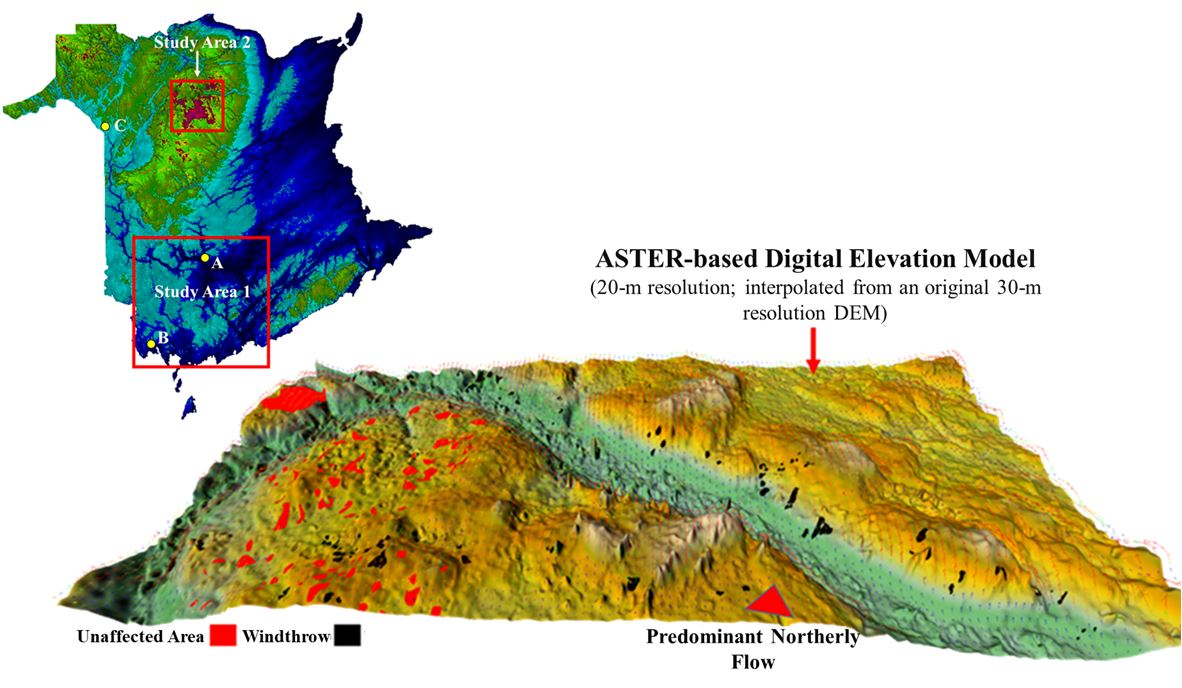
2.1. Study Areas

New Brunswick falls in the Atlantic Maritime Ecozone of eastern Canada (i.e., 44.59939° to 48.02186°N latitudes and 63.78114° to 69.05178°W longitudes; Figure 1), and is characterised by a fragmented landscape of predominantly forests and agriculture and variable terrain (i.e., elevations range from 0 to 834 m above mean sea level, AMSL). Forests occupy about 85% of the province’s land base, and agriculture occupies about 6%. Provincial climate is largely influenced by the region’s proximity to the Bay of Fundy in the south, the Northumberland Strait in the east and the Bay of Chaleur in the upper northeast corner of the province. On average, winters are milder than most regions of Canada. Springs are usually late and cool, and summers are moderate and breezy. The province experiences, on average, an annual mean air temperature and total precipitation between 2 °C and 7 °C and 1000 mm and 1360 mm, respectively [16].
Modelling the presence/absence of windthrow for bF and four other tree species was based on windthrow and non-windthrow data from southwestern NB (study area 1, Figure 1) for function development, and northcentral NB (study area 2, Figure 1) for function validation. Windthrow data in study areas 1 and 2 were based on outcomes of extratropical cyclone Arthur, July 4–5, 2014, and the Christmas Mountains windthrow event of November 7, 1994, respectively. Given the predominance of bF in the Christmas Mountains prior to the windthrow event, the function validation was feasible only for bF.

2.2. Surface Description and Development

The windthrow functions were constructed from data extracted from:
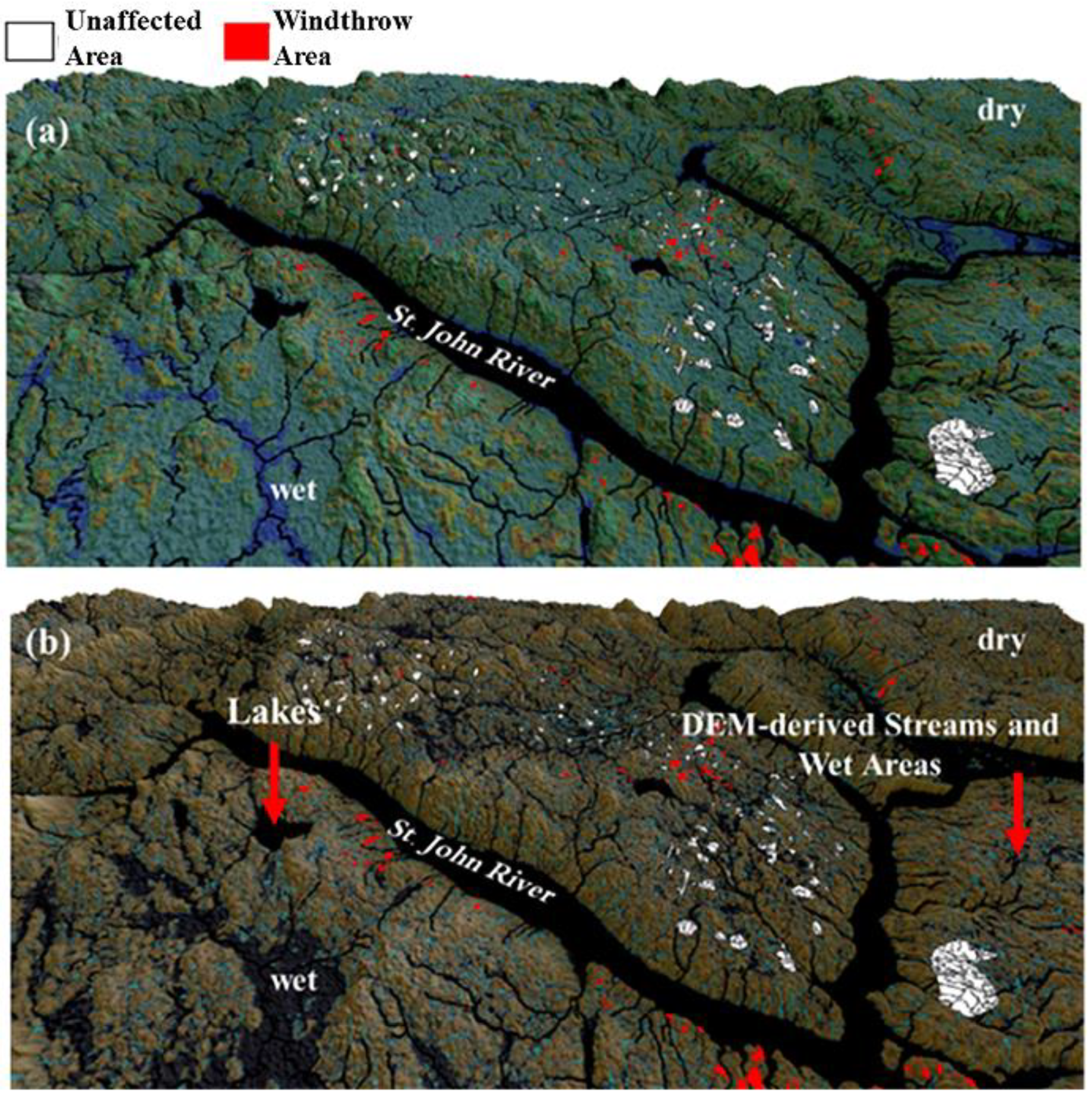
  • High-resolution, four-band digital orthophotos taken after the passage of extratropical cyclone Arthur in detection of windthrow- and non-windthrow-affected forests;
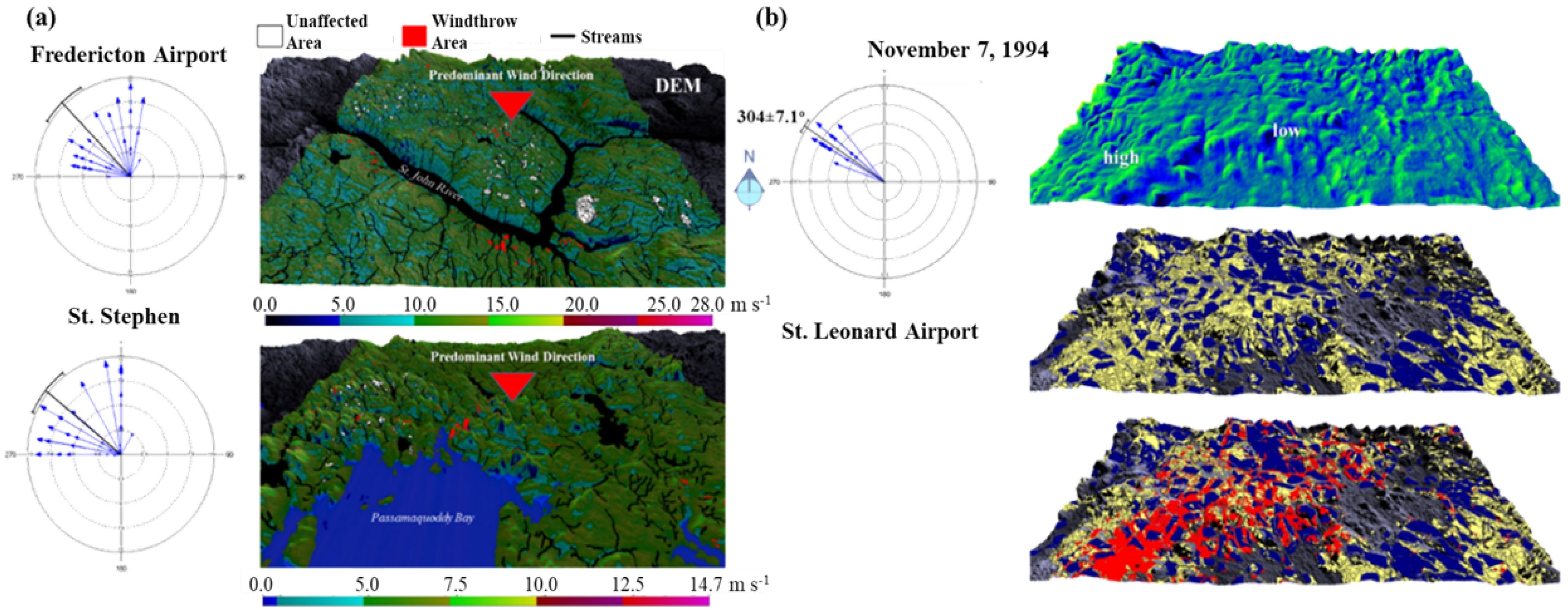
  • Spatially explicit reconstructions of wind fields during the peak of cyclone Arthur obtained with a computational fluid dynamics model (CFD) and input wind data (speed and direction) from two Environment and Climate Change Canada (ECCC) weather stations in southwestern NB (i.e., Fredericton Airport and St. Stephen weather stations; Figure 1);
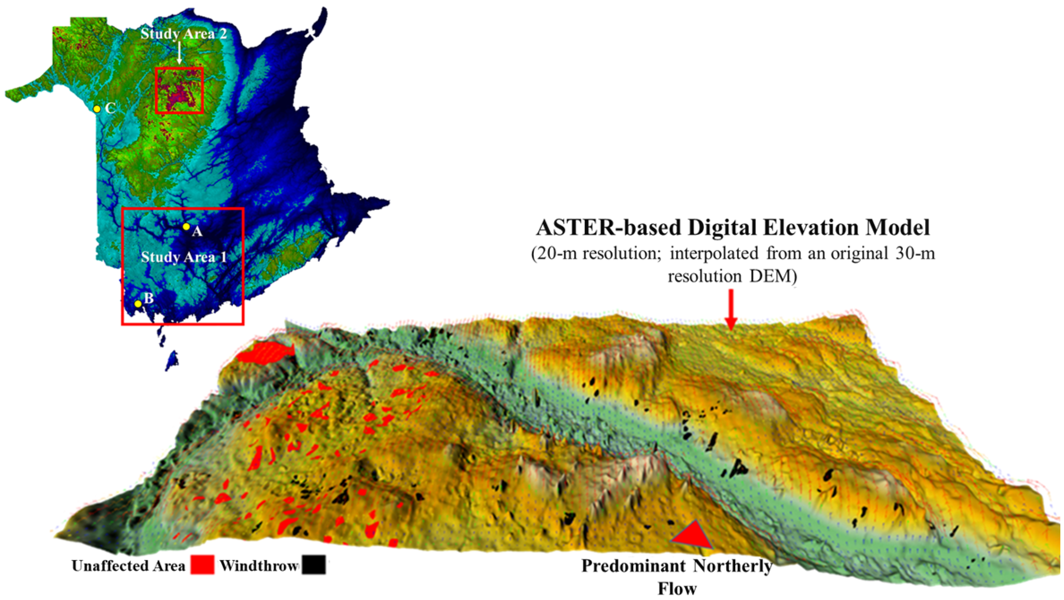
  • Selected forest-state variables from a suite of GIS-thematic variables of stand type, structure, soil depth and texture and other stand indicators (Table 1), and environmental site variables of digital elevation model (DEM)-derived estimates of slope, height above nearest drainage point [17,18] and modelled relative soil water content.
Principal component analysis (PCA) was subsequently used to reduce the number of variables from the suite of forest-state and site variables in developing the windthrow functions for bF and the other tree species.
The windthrow functions formulated for bF were later used to investigate the impact that current and future episodes (1950–2005 and 2006–2100) of extreme wind speeds may have on bF-dominated forests in NB. The future wind impact on bF was set in a context of anticipated species shift, as bF and other tree species will respond to changes in local temperature, precipitation, and soil water content over the next nine decades (based on past work by Bourque [22]). Climate-change scenarios for future environmental conditions for NB (i.e., temperature, precipitation, wind speed and direction) were based on 0.44° × 0.44°-resolution climate projections from ECCC’s most recent RCM (CanRCM4 [23]) developed by the Canadian Centre for Climate Modelling and Analysis (CCCma). CanRCM4 is driven by its parent global model (CanESM2 [24]) for all downscaling applications by employing spectral nudging in CanESM2. In our case, the simulations were based on two representative concentration pathways (RCP’s [25]) projected to contribute to a net additional global radiative forcing of 4.5 and 8.5 W m−2 by 2100 (RCP’s 4.5 and 8.5, respectively). The following sections describe the analytical procedures and input information (area extractions, for individual forest stands) used in developing the windthrow maps displayed throughout the paper.

2.3.1. Digital Elevation Model

The DEM of NB was based on the 30-m resolution Advanced Spaceborne Thermal Emission and Reflection Radiometer (ASTER) Global Digital Elevation Model ver. 2.0 (GDEM; http://asterweb.jpl.nasa.gov/gdem.asp, accessed on March, 2015) resampled at a 20-m resolution with bicubic interpolation (Figure 1). The DEM served as a data layer central to modelling the likelihood of windthrow province-wide under six extreme wind events.

2.3.2. Wind Speed and Direction

Wind speed and direction were modelled spatially according to the full three-dimensional Navier–Stokes equations, incorporating both the effects of atmospheric turbulence and thermal processes [26]. Computational fluid dynamics model [26] calculations of sustained maximum wind speed (Figure 2) for southwest (study area 1) and northcentral NB (study area 2; Figure 1) were based on a boundary-fitted coordinate system. Initial boundary conditions were specified by the near-surface air temperature and sustained wind speed and direction recorded at the Fredericton Airport and St. Stephen weather stations (Figure 1) during the peak of extratropical cyclone Arthur (mean air temperature of 14.4 °C and 13.5 °C and wind speed and direction of 23.2 m s−1 and 16.3 m s−1 and 0° from true north, respectively) and corresponding measurements recorded at the St. Leonard Airport weather station, upwind of the Christmas Mountains, for the Christmas Mountains windthrow event (mean air temperature of 0.5 °C and wind speed and direction of 13.0 m s−1 and 304°, respectively [16]). In both instances, a wind speed at 500 m AMSL was specified as corresponding to a mean value of 1.3 × near-surface sustained wind speed (after Franklin et al. [27]). Temperature stratification of the atmosphere was set to neutral for both wind events.
During a particular windstorm event, windthrow largely results from the destabilising forces generated by large-to-medium size eddies (wind gusts) formed as the prevailing airflow interacts with the underlying irregular terrain and surface cover. However, in this paper, we refer to sustained maximum wind speeds as the main indicator of windthrow, because (i) sustained wind speeds are always weaker then peak wind gusts (PWG’s); (ii) they are easier to model spatially with CFD-models and (iii) PWG’s, although intermittent, can be related empirically to sustained wind speeds (e.g., [28]). Peak wind gusts during sustained airflow over land were calculated here from sustained maximum wind speeds (η) and a wind-gust function formulated from wind speeds recorded during fifteen major mid-Atlantic hurricanes, including Hurricane Sandy [29], i.e.,
PWG s = [ 1 . 9506 0 . 173 ln ( η 0 . 44704 ) ] η ,
where η is the sustained maximum wind speed (m s−1). The denominator in the quotient in Equation (1), i.e., 0.44704, allows for a unit conversion from m s−1 to miles hour−1. The bracketed term in Equation (1) is the gust factor [29].

2.3.3. Soil Water Content

The height above nearest drainage point (Figure 3a) provides a simple static (time-independent) measure of potential drainage, particularly close to drainage channels [17,30], and is described as the vertical separation between raised dry land and a localised estimate of the water table level based on surface water defined by a GIS hydrological layer. For a particular dry cell, the wet cell nearest it is located by means of an iterative search algorithm that minimises the horizontal distance between the subject dry cell and the wet cell downslope, while taking into account DEM-specified flow directions and pathways [17,18]. Here, HNDP=0 m signifies visible surface water, whereas large HNDP’s signify low water tables and potentially drier soil conditions. In upland positions of landscapes, HNDP does poorly as an indicator of soil water content, as there is no realistic connection between HNDP and potentially variable soil water content. To avoid the challenge this presents, we introduced a water budget-based calculation of relative soil water content to improve the representation of soil water content in upland positions of landscapes. Because the water budget-based calculation of the variable depends on hydrometeorological inputs and outputs that may conceivably change over time, its calculations are time dependent.
Combining the two variables in a single representation of soil water content is acceptable, as HNDP approximates the influence on soil water content relative to the vertical distance to drainage points, whereas the soil water content module of Landscape Distribution of Soil moisture, Energy, and Temperature (LanDSET) [19,20] does better at representing soil water content relative to flow characteristics of the terrain (i.e., pathways and pooling locations), particularly in upland positions of the landscape. Together, HNDP and LanDSET-based calculations of relative soil water content have the potential to improve description of surface water flow-related processes and features across forested landscapes [18].
Steady-state values of relative soil water content of southwest (Figure 3b) and northcentral NB were estimated numerically, following methods described in several scientific articles central to the description of LanDSET [19,20,31,32]. LanDSET addresses soil water distribution according to a DEM cell-by-cell assessment of hydrological fluxes, including precipitation, evapotranspiration, percolation and surface runoff. The input to the model includes topography, by way of DEM elevations and cell size specification (20 m), net radiation balance and annual precipitation described spatially by numerical interpolation of annual precipitation recorded at 32 provincial weather stations. Prior to the calculation of relative soil water content, the raw DEM was processed by removing false depressions with the pit-filling algorithm of Planchon and Darboux [33], accessible in SAGA (System for Automated Geoscientific Analyses [34]).
The hydrological inputs to individual DEM gridpoints were precipitation and lateral flow from upslope regions, and outputs were percolation (deep seepage), evapotranspiration and surface runoff flows to regions downslope. Surface water on valley slopes was channelled downslope according to zones of confluence-divergence in the local landscape. The calculation of gridpoint evapotranspiration was based on an application of the Priestley–Taylor equation [35], gridpoint relative soil water content and LanDSET-model evaluation of net all-wave radiation [20]. The values of relative soil water content were in the range of 0.0–1.0, with 0.0 being associated with the drier sites at or below the permanent wilting point, and 1.0 with the wetter sites at or above field capacity. Percolation was based entirely on relative soil water content and occurs whenever soils are above field capacity [20]. Above field capacity, percolation rates were defined as a function of soil property and the saturated conductivity of the soil. The values for the equation parameters have been listed by Bourque et al. [19,20].

2.3.4. Windthrow Detection

The presence/absence of windthrow in study area 1 (Figure 1) was determined by photointerpretation of 30-cm resolution, colour infrared (CIR, surface reflectance-based) digital orthophotos (e.g., Figure 4) taken after the passing of extratropical cyclone Arthur. Individual bands in CIR imagery consist of a matrix of pixels representing colours in the red, green, blue (RGB) or near infrared (NIR) segments of the electromagnetic spectrum.
Living vegetation absorbs blue and red light to produce chlorophyll and drive photosynthesis. Healthy plants possess more chlorophyll and, as a result, reflect more NIR energy than damaged or dying plants. Consequently, evaluating a plant’s surface reflectance in terms of both absorbed and reflected visible light (Red Green Blue, RGB) and NIR energy can convey important diagnostic information about the plants’ physiological status.
In the false-colour image in Figure 4d (NIR+RG), light pink to greenish colours correspond to damaged and windblown trees and ground debris (e.g., fallen stems, dead detached foliage and branches and exposed forest floor), whereas bright red colours coincide with healthy, undamaged trees and foliage. Colour rendering of images to false colour, as demonstrated in Figure 4b,c, helps to locate windthrow-affected areas.

2.3.5. Windthrow Function Development

The windthrow functions were generated with genetic programming (GP)-driven logistic regression. Logistic regression is a statistical procedure widely used in classifying objects as either being present or absent (i.e., binary in nature), given a specific decision threshold value. Regression values below the threshold value signify absence (giving a value of 0.0), and values above the threshold signify presence (giving a value of 1.0). Here, absence refers to forest stands that are observed/predicted to have been left undamaged by wind, and presence refers to stands that are observed/predicted to have been damaged. All wind impact calculations were carried out at the DEM grid cell level and were not carried out for individual stands or soil formations. Information about stands and soil formations was passed on to individual grid cells by rasterising relevant feature classes (shapefiles) at the same resolution as the base DEM (i.e., at 20-m resolution).
Genetic programming-based regression is used to determine which nonredundant variables are particularly important in explaining variability in a dependent variable from the list of independent variables (Table 1), which, in our case, was the presence/absence of windthrow. Genetic programming-based regression is a procedure founded on evolutionary computation in search of algebraic equations by reducing the difference between target values and values calculated with the equations generated with the procedure [36]. Different from conventional regression, which determines parameter values of known equations, no specific mathematical expression is needed as a starting point with this approach. Rather, primary expressions are formed by randomly combining primitive, base functions of input variables (linear and nonlinear) with algebraic operators. Equations retained by the procedure are those that replicate the target output data better than others, and undesirable solutions are simply discarded. The procedure stops whenever the desired accuracy in data replication or level of machine learning has been reached.
A nontrivial problem in using GP-based methods is the amount of time sometimes required to arrive to an acceptable solution. One method to reduce GP-processing times is to reduce the number of input variables (Table 1) to a few important explanatory variables by means of data mining techniques, e.g., principal component analysis, regression tree analysis, cluster analysis, artificial neural networks and others [37]. Data reduction with any of these methods help to determine which input variables, among those being considered, explain the most variation in a dataset. Involving redundant and nonexplanatory variables in equation development simply helps to slow down solution convergence.
To help reduce problem dimensionality, we employed principal component analysis (PCA) on the suite of forest-state and environmental-site variables addressed in Table 1. Principal component analysis groups redundant variables under a principal component (or primary axis), with each component explaining a portion of the variation in the dataset. Variables grouped together after rotation of the primary axes (based on the VARIMAX-option in SYSTAT ver. 11) are viewed to contain very similar information. As a result, only one of these variables with highest factor loading or easiest to quantify or measure needs to be retained, and all other variables belonging to the same principal component are ignored. For a particular dataset, the number of viable principal components depends on the eigenvalue produced during axis rotation. Principal components, with an eigenvalue > 1.0, collectively explain the majority of the variation in the dataset.

2.3.6. Projected Future Climates

Future climate change scenarios for NB were based on ECCC’s RCM projections (i.e., CanRCM4_CanESM2 at 0.44° × 0.44° resolution) based on RCP’s 4.5 and 8.5 [25]. RCP 4.5 represents a scenario that stabilises a net rise in global radiative forcing to 4.5 W m−2 prior to the end of the 21st century. This scenario assumes that global annual greenhouse gas emissions peak around 2040, and then decline with the implementation of new technology [25], whereas RCP 8.5 represents a significantly more intensive scenario of rising global radiative forcing, reaching 8.5 W m−2 by the end of the 21st century. RCP 8.5 assumes global emissions continue to increase corresponding to the pathway with the greatest greenhouse gas emissions [38].
Figure 5 gives province-wide windspeed frequencies as a function of RCM-modelled historical climatic regime (1950–2005; inset to Figure 5a) and seasonal wind for two locations in NB (Figure 5b), i.e., one inland location on the southern boundary of study area 2 (gridpoint 61, near the Christmas Mountains) and one coastal location, near Miscou Island, NB (gridpoint 94; see inset to Figure 5a). There was significant deviation (climatology) in overall wind speeds between the two locations. The sustained maximum wind speeds in coastal areas had a greater chance of exceeding 9 m s−1, attaining wind gusts > 13 m s−1, particularly during winter, due to stronger atmospheric circulation.
Wind directions were predominantly from the northeast and south in proximity to the eastern and southern coast of NB, and west-to-northwest direction in northcentral NB.
The province-wide evaluation of windstorm impact on bF stands for both historical and future climate scenarios (Figure 6) was based on six one-time events (two historical and four future events) of RCM-generated maximum wind speed over 56 (historical data) to 95 years (future data) at both inland and coastal areas of NB (gridpoints 61 and 94, respectively; Figure 5a). Given the computational grid area and time limitations of CFD models, achieving the level of spatial detail required for windthrow calculations at 20-m resolution for the entire province was enormously challenging. As an effective sidestep to this problem, we instead enhanced the province-wide RCM-based maximum wind speeds using the statistical downscaling of associated corrections (dependent variable) derived by dividing gridpoint CFD- and RCM-based maximum wind speeds occurring within study area 2. The independent variables to the procedure included RCM-based wind speeds and four DEM terrain-based indices, including wind-effect index, terrain ruggedness index, point maximal curvature and relative elevation. The wind-effect index is a nondimensional quantity that defines the areas of the landscape either exposed to or sheltered from high wind speeds by taking into account spatial variation in digital terrain elevations and interpolated RCM wind speeds and directions using SAGA. The statistical relation of windspeed correction is subsequently used to produce province-wide estimates of windspeed correction based on province-wide surfaces of independent variables at 20-m resolution, serving as inputs. Windspeed corrections are then multiplied to the interpolated RCM-generated wind speeds, increasing their overall spatial resolution.

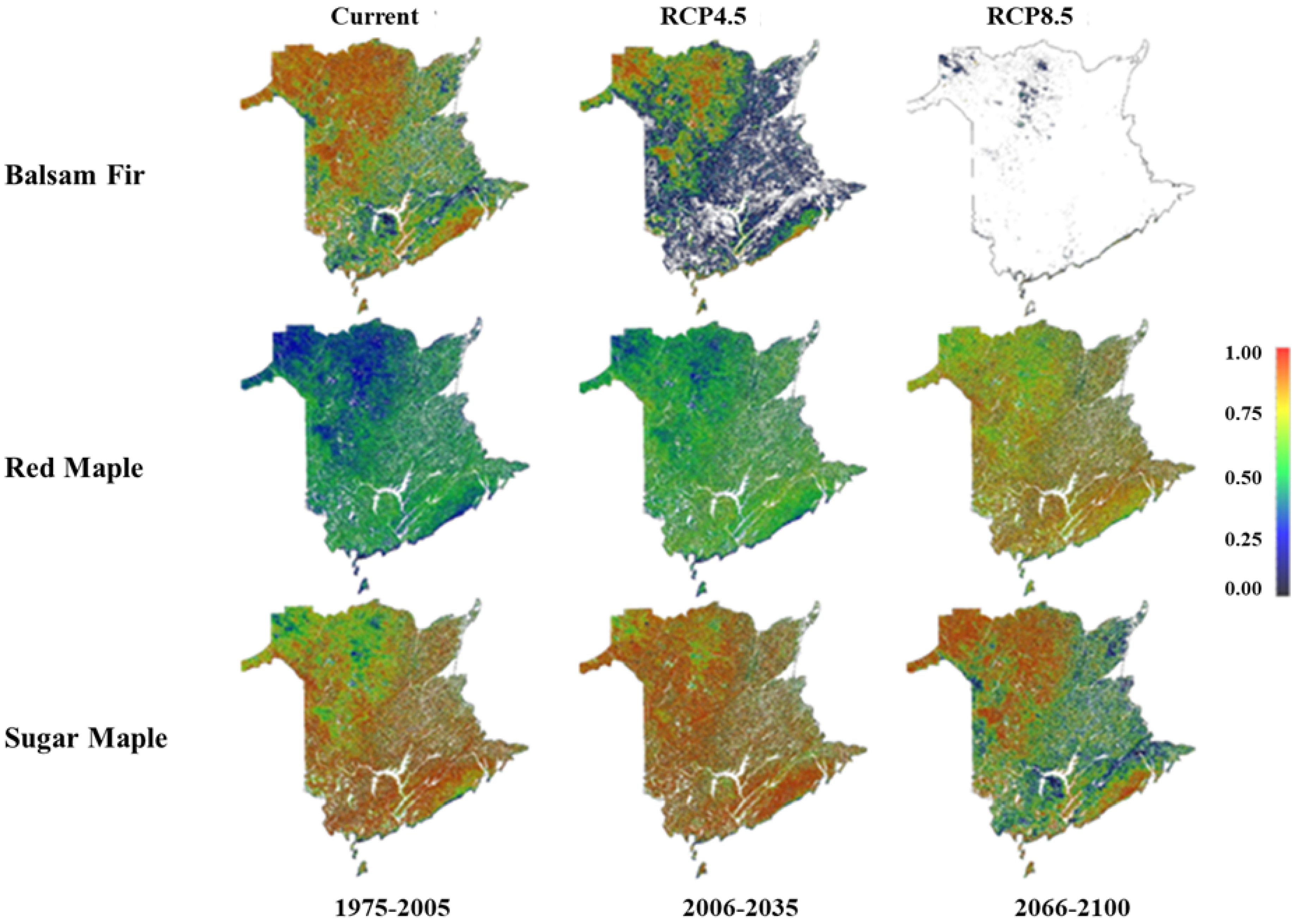
2.3.7. Projected Species Shifts

The discussion of province-wide wind impact on bF stands was done in a context of anticipated species shift, as individual bF trees are expected to respond to changes in local temperature, precipitation and soil water content over the next nine decades (i.e., 2006–2100) for future climate scenarios, RCP’s 4.5 and 8.5.

3. Results and Discussion

3.1. Principal Component Analysis

Table 2 provides the factor loadings associated with the application of PCA to the full set of variables listed in Table 1. From this analysis, eight principal components (PC’s) with eigenvalues > 1.0 were identified. Collectively, the PC’s explained 79% of the variance in the dataset. Given group membership, factor loadings (Table 2) and the ease to which variables can be quantified spatially, mean height above nearest drainage (HNDP_MEAN), relative soil water content (SWC_MEAN), wind speed (WNDSPD_MEAN), density class (DC), tree form (TREEFORM), soil depth (SDEPTH) and mean slope (SLP_MEAN) were judged to be the most important explanatory variables, with HNDP_MEAN explaining the greatest variation (14.2%) in the data among the seven variables, followed by wind speed (13.5%; Table 2). Beyond these seven variables, the remaining variables in Table 1 were discounted from further consideration.

3.2. Windthrow Function Development

Windthrow equation for bF and associated thresholds (δi, i=1,…,4 and decision thresholds) were derived from GP-based regression (Table A1 and Table A2 in Appendix A; these Tables give the windthrow equations and thresholds associated with bF and the other tree species). The windthrow function for bF (Table A1) was able to correctly classify the majority of windthrow- and non-windthrow-affected stands during function development. The area under the receiver operating characteristic (ROC) curve for bF exceeded 94% (Table A2), with a sample size of 518 of windthrow- and non-windthrow-affected stands. An area under the ROC-curve of 100% indicates a perfect match between observed and predicted outcomes. Here, WNDSPD, HNDP, SWC and SLP refer to their respective means (Table 1). The windthrow-functions for the other tree species (Table A1) performed equally well with determining outcomes of windthrow, despite being based on smaller sample sizes (Table A2).
Relative to the other tree species, bF is particularly vulnerable to blowdown because of the species’ shallow rooting habit particularly in shallow, wet soils. This is supported by the relatively low critical wind speed determined for the species during regression, i.e., 5.8 m s−1 compared to 7.0 m s−1 and 9.5 m s−1 for red and sugar maple (Table A2). Estimated PWG’s of 8.8 m s−1, 10.3 m s−1 and 13.5 m s−1 were associated with the calculated critical wind speeds of 5.8 m s−1, 7.0 m s−1 and 9.5 m s−1. Red and sugar maple tended to have deeper rooting systems, particularly in well-drained, deep upland soils as a result of being more strongly anchored. These findings are consistent with other researchers’ findings based on different methods of evaluation. For example, after a catastrophic wind event in the Charlevoix region of Quebec, Ruel [39] found that 62% of the total windthrow was located in bF stands. For wind speeds between 7.8–10.3 m s−1, bF stands were more heavily damaged than mixed black spruce stands. In a study of experts’ perceptions of windthrow, experts consistently ranked bF, among thirteen northern temperate tree species, including seven hardwood and six softwood species, as especially prone to windthrow [40]. Burns and Honkala [41] also placed bF as not being very resistant to windthrow. Canham et al. [42] have reported that red maple was generally less windfirm than sugar maple. Our results are consistent with that observation (Table A2).

3.3. Windthrow Function Validation

The windthrow function for bF was subsequently validated against windthrow data acquired from the Christmas Mountains blowdown event (Figure 7). Overall, the prediction of windthrow-affected areas in the Christmas Mountains (study area 2; Figure 1) agreed fairly well with the windthrow sites identified from photointerpretation (Figure 7b), as 93.3% of the impact zone established through photointerpretation corresponded with predictions of the occurrence of windthrow. Unmatched areas outside the impact zone indicated the possibility of windthrow having actually occurred based on the prediction of occurrence, although they were not flagged as containing windthrow. On closer inspection of mostly cloud-free infrared and optical-based Landsat images taken before and after windthrow (i.e., September 21, 1994 and June 4, 1995) and higher-resolution, coloured aerial film photographs taken after windthrow (August 08, 1995), all 25 additional locations that showed a high likelihood of windthrow possessed some level of windthrow but at varying degrees of destruction. In general, the occurrence of windthrow in the Christmas Mountains was more pronounced in areas (i) with shallow soils (SDEPTH class 2, soils 30–65-cm deep; Figure 7c), even in landscape locations of moderate sustained wind speeds (~6 m s−1), and (ii) exposed to localised, terrain-induced accelerations in mean airflow and moderate-to-strong wind gusts (> 9 m s−1, based on Equation (1)).

3.4. Projected Windthrow under Current and Future Climatic Conditions

Figure 8 gives the projected windthrow areas and associated maximum wind speeds for NB under current and future extreme wind conditions associated with two 56-year- and four 95-year-classed extreme wind events for historical and future climate scenarios, assuming no net change in tree species distribution from current conditions. Windthrow under these projected wind events are expected to occur most strongly in the northcentral highlands and along the eastern coast of the province (red-coloured areas), where wind speeds are projected to be consistently stronger. Because high winds are common in mountainous terrain and along coastal areas due to atmospheric compression in elevated terrain and strong thermal gradients between land and water, many of the bF in these areas could conceivably become wind-firmed over their lifetime and, as a result, develop resistance to overturning in moderate-to-strong winds. Of course, the level of detail this presents is generally outside our capabilities to model with full confidence.
The tendency for elevated windthrow in the NB highlands and regions closer to the coast did not change significantly with prevailing wind direction during the extreme wind events considered in this study. Maximum wind speeds in inland locations of NB are projected to exhibit minor changes over the next nine decades, with an average increase of about 0.037% per year compared to what is being predicted for coastal areas of the province, i.e., +0.066% per year. Although a temporary minor decline in wind speeds is projected for inland locations during the first 30 years under the RCP 8.5 climate scenario, small increases are projected for the remainder of the time.
It is very unlikely that the projections illustrated in Figure 8 are reliable, especially when viewed at the individual stand level. Statistical downscaling of RCM-generated wind speeds may capture some macroscale features of the landscape (e.g., mountainous and near-coastal features) as shown in Figure 8, but the smaller-scaled features within these areas are generally too small to distinguish, especially considering that input wind speeds used in statistical downscaling (Figure 6) are from computations performed at coarse spatial resolutions, i.e., ~50-km resolution, as compared to the 20-m target resolution. CFD-based wind models can capture some of this spatial variability as demonstrated in Figure 7a, but its grid-area limitations, due to its exorbitant need of computer random access memory and processing time, render these types of models unsuitable for large DEMs at subhectare resolutions. As a compromise, we can view the probability of windthrow as a function of normalised ranking of statistically downscaled wind speeds, similar to the logistic density function addressed in Figure 7. Stands with a value of 1.0, indicating highest possible sustained maximum wind speeds > 20 m s−1 with PWG’s > 26 m s−1, are expected to produce windthrow compared to stands with a lower probability of windthrow under lower wind speeds (captured in blue).
As bF habitat and bF retreats northward because of net increases in growing-season degree-days and increases in soil water content, the presence of bF and, therefore, windthrow in bF is anticipated to decline over the next nine decades (Figure 9). The rate of bF decline province-wide is expected to vary subject to differences in topography (low (warmer) vs. high-elevation areas (cooler)), growing degree-day sums and soil moisture. This decline is particularly pronounced for the RCP 8.5 climate scenario (associated with a net increase of 5.4 °C in summer over the 2081–2100 period, with respect to the 1986–2005 reference period), whereby 95.6% of viable bF habitat is expected to be lost by 2100 under RCP 8.5 (Figure 9) compared to 50.9% under RCP 4.5. Increases in soil water content in already shallow soils, particularly in saturated-prone areas of the landscape (e.g., channel depressions), can further increase the risk of windthrow by restricting tree root growth (and anchoring potential) even more. The distribution of red and sugar maple habitat is expected to expand with a province-wide amelioration of growing conditions for the two species (Figure 9). The replacement of bF with windfirm hardwood species, like the maples, has the potential to elicit substantial shifts in forest composition and wind firmness in future NB forests.
In situations where frozen soils provide additional anchoring for many of the trees, an incremental shift toward higher winter temperatures (net increase of 6.4 °C in winter over the 2081–2100 period; Figure 10) may result in greater windthrow in winter, especially in areas of the province that are particularly susceptible to strong westerly and northwesterly winds common to the interior highlands of the province and northeastly winds for remote landward locations close to the eastern coast of NB (Figure 6). With an abundance of snow on the ground in Atlantic Canada, soils in highly-to-moderately dense coniferous forests are seldom frozen to any great depths during the snow-accumulation period of the year (Figure 10) because of the insulating properties of both the overstorey vegetation and snow layer and the upward transfer of heat in seasonally cooling and snow-covered soils (Figure 10b). Consequently, coniferous forests, including bF forests in NB, rarely benefit from added anchoring in winter. Future lowering of the snowpack as winter air temperatures shift upward (Figure 10c,d) may cause midwinter thaw-refreeze events and cavitation in stemwood-porous species to occur, particularly in the maples and birches, which may predispose these species to dieback [43] and, thus, to stem-breakage and windthrow. This effect, however, will gradually dissipate in the future (e.g., 2070–2100) as air temperatures continue to climb and freezing of the soil complex is potentially confined to a very shallow depth of the forest floor (Figure 10d). In their study, Saad et al. [44] found an overall increased risk of windthrow in bF forests in eastern Canada for the future (by 3% to 30%) mostly as a result of an increased duration of unfrozen soil conditions by the end of the 21st century under an RCP 8.5 climate scenario. Their windthrow projections for Atlantic Canada, however, do not account for the ongoing and projected erosion of bF growing conditions (habitat) in the region with continued climatic warming.

4. Conclusions

In this paper, we present a set of windthrow equations used to determine the presence/absence of windthrow in NB forests assessed from remote sensing following episodes of hurricane-strength winds. The system integrates the binary calculation of windthrow to modelled biophysical surfaces of wind speed, forest state (density and size classes) and site soil conditions (soil depth, soil water content, slope) through genetic-programming-driven logistic regression. Results from a validation of the windthrow function for bF showed reasonable agreement between modelled and photointerpreted areas of windthrow in the Christmas Mountains following a major windstorm. From a wind firmness point of view, bF is the least resistant to windthrow when confronted with moderate-to-strong winds. This is illustrated by the relatively low critical wind speeds needed to initiate windthrow in bF stands, compared to other tree species, such as the maples.
Maximum wind speeds are expected to increase throughout NB over the next nine decades, but at nominal rates, i.e., 0.066 vs. 0.037% per year under climate-scenario RCP 8.5 for coastal and inland locations. Because coastal winds are generally stronger most of the time, due to strong thermal gradients between land and water, the net increase in maximum wind speeds by the end of the 21st-century is expected to be greatest for coastal areas of the province. Inland areas of NB will see much lower increases overall. The predominance of windthrow in currently existing bF stands in NB is expected to be moderated in the future, as the species responds to an overall decline in viable growing conditions with increased temperatures and soil moisture, and a gradual physiological and structural weakening of residual bF. Windfirm hardwood species are likely to replace bF as it progressively withdraws from NB, potentially causing future, transitioning forests in NB to be more resistant to windthrow.
Given the range of natural climate variability and uncertainties regarding future greenhouse-gas emission pathways and climate response, changes projected by one climate model, or one emission scenario, should not be used in isolation (e.g., [46]). A range of projections from multiple climate models (ensembles) and emission scenarios is therefore a way to consider (a good practice to identify the main sources of uncertainties), especially when regional or local climate variables as maximum wind speed and wind gusts are concerned. There is low confidence in the projection of regional storm track changes, and the impact of such changes on regional surface climate from global climate models (e.g., [46]). There is a clear need to assess more regional and local scale windstorm changes using high-resolution information (i.e., finer than 50 km) from RCM’s. This is true for both extratropical and tropical cyclones that affect the maritime areas over the major part of the year. This will help confirm the outcomes of our study and provide improved risk assessments of windthrow in all tree species.

Author Contributions

Conceptualization, C.P.-A.B. and P.G.; methodology, C.P.-A.B. and J.I.M.; software, C.P.-A.B.; validation, C.P.-A.B., P.G., B.R.M., and J.I.M.; formal analysis, C.P.-A.B.; investigation, C.P.-A.B., P.G. and J.I.M.; resources, C.P.-A.B., P.G. and J.I.M.; data curation, C.P.-A.B. and P.G.; writing—original draft preparation, C.P.-A.B. and B.R.M.; writing—review and editing, C.P.-A.B., P.G., B.R.M., and J.I.M.; visualization, C.P.-A.B. and B.R.M.; supervision, C.P.-A.B.; project administration, C.P.-A.B.; funding acquisition, C.P.-A.B. and J.I.M. All authors have read and agreed to the published version of the manuscript.

Funding

This study was funded by the Environmental Trust Fund of the Government of New Brunswick (NB), Department of Environment and Local Government (NB DELG). The APC was funded by the Natural Sciences and Engineering Research Council of Canada.

Acknowledgments

We are grateful to Jeff Hoyt, NB DELG, for his unrelenting support of this project. We would like to acknowledge the National Aeronautics and Space Administration (NASA) for providing the ASTER-based digital elevation model free of charge and Dr. Paul Arp in our implementation of the ForHyM-model in developing Figure 10c,d. We would also like to thank Dr.’s Scinocca and Yanjun Jiao from CCCma/ECCC who provided the required information and output files from CanRCM4.

Conflicts of Interest

The authors declare no conflict of interest.

Appendix A. (Follows below, in Landscape Format)

Table A1. Windthrow functions, p(ϕk), for five native tree species of southwest New Brunswick based; δ 1 = { 1 , WS > η crit 0 , otherwise , where ηcrit is the critical sustained wind speed (m s−1), below which windthrow is very unlikely to occur. The critical wind speed is determined numerically from windthrow and CFD-modelled wind data associated with extratropical cyclone Arthur, July 4–5, 2014.
Speciesp(ϕk)1,2δ23δ3δ4
Balsam Fir δ 1 1.0 + 0.002 exp { 9.2 [ ( sin ( 69.0 HNDP ) 9.2 SWC 2 SLP 23.4 ) + δ 2 δ 3 δ 4 ] } SWC < 0.7 [ HNDP + 9 . 2 SWC 2 + cos ( 69.0 HNDP ) ] < SLP 4.3 max ( SWC , ( SLP 23.4 ) ) < SD
Black Spruce δ 1 1.0 + exp { 829 1.5 × 10 3 δ 2 min [ DC min ( 0.3 SLP , HNDP ) , cos [ cos ( 0.3 SLP ) ] ] } , min ( SLP 7.6 , 8 ) < SWC ( SLP 7.6 )
Eastern White Cedar δ 1 1.0 + exp { 385 395 max [ sin ( HNDP ( 47.8 2.1 HNDP ) ) , cos ( 0.3 HNDP ( SLP 4.3 HNDP ) ) ] }
Red Maple δ 1 1.0 + exp { 81.0 120.3 sin [ HNDP min ( 14.9 , max ( 8.2 , SLP ) ) δ 2 + HNDP + sin ( 1.5 SLP ) δ 3 ] } SWC < 0.5 HNDP < ( DC 1.1 )
Sugar Maple δ 1 1.0 + exp { 430 ( SWC + HNDP ) 10.4 + sin ( 5.9 + SWC + HNDP ) sin ( SD ) δ 2 751 } ( 0.3 + HNDP ) sin ( HNDP ) < DC
1 p(ϕk)-values < threshold (Table A2) denote stands predicted to be unaffected by windthrow, whereas p(ϕk)-values > threshold, stands predicted to have sustained some level of windthrow; 2 independent variables in windthrow-function definition: DC is the dominant-layer density class from 1–5, where 1 = number of stems up to 600 (merchantable) or up to 5000 (unmerchantable), 2 = number of stems up to 601–1200 (merchantable) or up to 5001–10,000 (unmerchantable), 3 = number of stems >1200 (merchantable) or 10,001–20,000 (unmerchantable), 4 = number of stems 20,001–30,000 (unmerchantable) and 5 = number of stems > 30,000 (unmerchantable; NB DNR Data Dictionary, 2004); HNDP is the height above nearest drainage point (m); SD is the soil-depth class (same as SDEPTH in Table 1 and Table 2 in the main body of the manuscript) from 1–4, where 1= < 30 cm, 2=30–65 cm, 3=65–100 cm and 4= >100 cm; SLP is the mean slope (SLP_MEAN) of the local terrain (°); SWC is the mean relative soil water content (SWC_MEAN) that ranges from 0–1, where 0 represents the permanent wilting point and 1, at field capacity; and WS is the mean wind speed (WNDSPD_MEAN) in m s−1; 3 δi’s (i=2,…,4) are several variable functions, evaluated at exactly 1.0, when conditions in columns 3–5 are satisfied and 0.0, otherwise.
Table A2. Input records and results from windthrow-function generation with nonlinear, logistic regression. Results include function accuracy, critical sustained wind speeds, decision thresholds and number of observations used in function formulation (Table A1); ηcrit (species’ critical windspeed requirement for windthrow) and decision thresholds are set during regression.
Tree SpeciesAccuracy 1
(%)
ηcrit
(m s−1)
Peak Wind Gust Associated with ηcrit 2
(m s−1)
Threshold
(unitless)
Number of Observations
Balsam Fir 94.65.88.80.03518
Black Spruce~1006.49.6 0.49129
Eastern White Cedar 93.45.88.80.02332
Red Maple 96.37.010.30.02243
Sugar Maple ~1009.513.50.50112
1 % accuracy is defined as the area under the receiver operating characteristic curve; 2 calculations of peak wind gusts are based on eqn. (1) in the main text.

References

  1. Ulanova, N.G. The effects of windthrow on forests at different spatial scales: A review. For. Ecol. Manag. 2000, 135, 157–167. [Google Scholar] [CrossRef]
  2. Klaus, M.; Holsten, A.; Hostert, P.; Kropp, J.P. Integrated methodology to assess windthrow impacts on forest stands under climate change. For. Ecol. Manag. 2011, 261, 1799–1810. [Google Scholar] [CrossRef]
  3. Jackson, T.; Shenkin, A.; Kalyan, B.; Zionts, J.; Calders, K.; Origo, N.; Disney, M.; Burt, A.; Raumonen, P.; Malhi, Y. A new architectural perspective on wind damage in a natural forest. Front. For. Global Chang. 2019, 1, 13. [Google Scholar]
  4. Quine, C.; Coutts, M.; Gardiner, B.; Pyatt, G. Forests and wind: Management to minimise damage. For. Comm. Bull 1995, 114, 24. [Google Scholar]
  5. Repap New Brunswick. The Christmas Mountains Blowdown; Miramichi, N.B., Ed.; Repap Training Centre: Miramichi, NB, Canada, 1995. [Google Scholar]
  6. Mitchell, S.J. Wind as a natural disturbance agent in forests: A synthesis. Forestry 2013, 86, 147–157. [Google Scholar] [CrossRef] [Green Version]
  7. Anyomi, K.A.; Mitchell, S.J.; Ruel, J.-C. Windthrow modelling in old-growth and multi-layered boreal forests. Ecol. Model. 2016, 327, 105–114. [Google Scholar] [CrossRef]
  8. Mokroš, M.; Výboštok, J.; Merganič, J.; Hollaus, M.; Barton, I.; Koreň, M.; Tomaštík, J.; Čerňava, J. Early stage forest windthrow estimation based on unmanned aircraft system imagery. Forests 2017, 8, 306. [Google Scholar] [CrossRef] [Green Version]
  9. Meng, J.; Bai, Y.; Ma, W. A management tool for reducing the potential risk of windthrow for coastal Casuarina equisetifolia L. stands on Hainan Island, China. Euro. J. For. Res. 2017, 136, 543–554. [Google Scholar] [CrossRef]
  10. Coates, K.D.; Burton, P.J. A gap-based approach for development of silvicultural systems to address ecosystem management objectives. For. Ecol. Manag. 1997, 99, 337–354. [Google Scholar] [CrossRef]
  11. Peringer, A.; Buttler, A.; Gillet, F.; Pătru-Stupariu, I.; Schulze, K.A.; Stupariu, M.-S.; Rosenthal, G. Disturbance-grazer-vegetation interactions maintain habitat diversity in mountain pasture-woodlands. Ecol. Model. 2017, 358, 301–310. [Google Scholar] [CrossRef]
  12. Anyomi, K.A.; Mitchell, S.J.; Perera, A.H.; Ruel, J.-C. Windthrow dynamics in Boreal Ontario: A simulation of the vulnerability of several stand types across a range of wind speeds. Forests 2017, 8, 233. [Google Scholar] [CrossRef] [Green Version]
  13. Raymond, P.; Bédard, S. The irregular shelterwood system as an alternative to clearcutting to achieve compositional and structural objectives in temperate mixedwood stands. For. Ecol. Manag. 2017, 398, 91–100. [Google Scholar] [CrossRef]
  14. Wilson, E.A.; Maclean, D.A. Windthrow and growth response following a spruce budworm inspired, variable retention harvest in New Brunswick, Canada. Can. J. For. Res. 2015, 45, 659–666. [Google Scholar] [CrossRef]
  15. Jaloviar, P.; Saniga, M.; Kucbel, S.; Pittner, J.; Vencurik, J.; Dovciak, M. Seven decades of change in a European old-growth forest following a stand-replacing wind disturbance: A long-term case study. For. Ecol. Manag. 2017, 399, 197–205. [Google Scholar] [CrossRef]
  16. Environment and Climate Change Canada, Historical Data. Available online: https://climate.weather.gc.ca/ (accessed on 12 March 2020).
  17. Rennó, C.D.; Nobre, A.D.; Cuartas, L.A.; Soares, J.V.; Hodnett, M.G.; Tomasella, J. HAND, a new terrain descriptor using SRTM-DEM: Mapping terra-firme rainforest environments in Amazonia. Remote Sens. Environ. 2008, 112, 3469–3481. [Google Scholar] [CrossRef]
  18. Murphy, P.N.C.; Ogilvie, J.; Meng, F.R.; White, B.; Bhatti, J.S.; Arp, P.A. Modelling and mapping topographic variations in forest soils at high resolution: A case study. Ecol. Model. 2011, 222, 2314–2332. [Google Scholar] [CrossRef]
  19. Bourque, C.P.-A.; Gullison, J.J. A technique to predict hourly potential solar radiation and temperature for a mostly unmonitored area in the Cape Breton Highlands. Can. J. Soil. Sci. 1998, 78, 409–420. [Google Scholar] [CrossRef]
  20. Bourque, C.P.-A.; Meng, F.-R.; Gullison, J.J.; Bridgland, J. Biophysical and potential vegetation growth surfaces for a small watershed in northern Cape Breton Island, Nova Scotia, Canada. Can. J. For. Res. 2000, 30, 1179–1195. [Google Scholar] [CrossRef]
  21. Fahmy, S.H.; Hann, S.W.R.; Jiao, Y. Soils of New Brunswick: The Second Approximation; Agriculture and Agri-food Canada Report, Technical Publication Number, NBSWCC-PRC 2010-01; Eastern Canada Soil and Water Conservation Centre and Agriculture and Agri-food Canada: Moncton, NB, Canada, 2010; p. 87. [Google Scholar]
  22. Bourque, C.P.-A. Modelled Potential Tree Species Distribution for Current and Projected Future Climates for New Brunswick, Canada; Unpublished Report Prepared for the New Brunswick Department of Environment and Local Government: Fredericton, NB, Canada, 2015; p. 40.
  23. Scinocca, J.F.; Kharin, V.V.; Jiao, Y.; Qian, M.W.; Lazare, M.; Solheim, L.; Flato, G.M.; Biner, S.; Desgagne, M.; Dugas, B. Coordinated global and regional climate modeling. J. Clim. 2016, 29, 17–35. [Google Scholar] [CrossRef]
  24. Arora, V.K.; Scinocca, J.F.; Boer, G.J.; Christian, J.R.; Denman, K.L.; Flato, G.M.; Kharin, V.V.; Lee, W.G.; Merryfield, W.J. Carbon emission limits required to satisfy future representative concentration pathways of greenhouse gases. Geophys. Res. Lett. 2011, 38, L05805. [Google Scholar] [CrossRef]
  25. Van Vuuren, D.P.; Edmonds, J.; Kainuma, M.; Riahi, K.; Thomson, A.; Hibbard, K.; Hurtt, G.C.; Kram, T.; Krey, V.; Lamarque, J.-F.; et al. The representative concentration pathways: An overview. Clim. Chang. 2011, 109, 5–31. [Google Scholar] [CrossRef]
  26. Lopes, A.M.G. WindStation—A software for the simulation of atmospheric flows over complex topography. Environ. Modell. Softw. 2003, 18, 81–96. [Google Scholar] [CrossRef]
  27. Franklin, J.L.; Black, M.L.; Valde, K. GPS dropwindsonde wind profiles in hurricanes and their operational implications. Weather Forecast. 2002, 18, 32–44. [Google Scholar] [CrossRef]
  28. Tyner, B.; Aiyyer, A.; Blaes, J.L.; Hawkins, D.R. An examination of wind decay, sustained wind speed forecasts, and gust factors for recent tropical cyclones in the mid-Atlantic region of the United States. Weather Forecast. 2015, 30, 153–176. [Google Scholar] [CrossRef]
  29. Blaes, J.L.; Hawkins, R.D. Improving Methodologies for Operational Forecasts of Winds and Wind Gusts during Tropical Cyclones. Available online: https://vlab.ncep.noaa.gov/documents/10157/137122/20160316.vlab.presentation.pdf/a78e0a31-0036-483c-8623-3d7f7d6a0e9f (accessed on 3 March 2020).
  30. Schietti, J.; Emilio, T.; Rennó, C.D.; Drucker, D.P.; Costa, F.R.C.; Nogueira, A.; Baccaro, F.B.; Figueiredo, F.; Castilho, C.V.; Kinupp, V.; et al. Vertical distance from drainage drives floristic composition changes in an Amazonian rainforest. Plant Ecol. Divers. 2014, 7, 241–253. [Google Scholar] [CrossRef]
  31. Moore, I.D.; Norton, T.W.; Williams, J.E. Modelling environmental heterogeneity in forested landscapes. J. Hydrol. 1993, 150, 717–747. [Google Scholar] [CrossRef]
  32. Gallant, J. Complex Wetness Index Calculations, WET Documentation Ver. 2.0.; Centre for Resource and Environmental Studies, Australian National University: Canberra, Australia, 1996. [Google Scholar]
  33. Planchon, O.; Darboux, F. A fast, simple and versatile algorithm to fill the depressions of digital elevation models. Catena 2001, 46, 159–176. [Google Scholar] [CrossRef]
  34. Conrad, O.; Bechtel, B.; Bock, M.; Dietrich, H.; Fischer, E.; Gerlitz, L.; Wehberg, J.; Wichmann, V.; Böhner, J. System for automated geoscientific analyses (SAGA) v. 2.1.4. Geosci. Model. Develop. 2015, 8, 1991–2007. [Google Scholar] [CrossRef] [Green Version]
  35. Priestley, C.H.B.; Taylor, R.J. On the assessment of surface heat flux and evaporation using large scale parameters. Mon. Weather Rev. 1972, 100, 81–92. [Google Scholar] [CrossRef]
  36. Schmidt, M.; Lipson, H. Distilling free-form natural laws from experimental data. Science 2009, 324, 81–85. [Google Scholar] [CrossRef]
  37. Cios, K.J.; Pedrycz, W.; Swiniarski, R.W.; Kurgan, L.A. Data Mining: A Knowledge Discovery Approach; Springer: New York, NY, USA, 2007; p. 606. [Google Scholar]
  38. Riahi, K.; Rao, S.; Krey, V.; Cho, C.; Chirkov, V.; Fischer, G.; Kindermann, G.; Nakicenovic, N.; Rafa, J.P. RCP 8.5—A scenario of comparatively high greenhouse gas emissions. Clim. Chang. 2011, 109, 33–57. [Google Scholar] [CrossRef] [Green Version]
  39. Ruel, J.C. Factors influencing windthrow in balsam fir forests: From landscape studies to individual tree studies. For. Ecol. Manag. 2000, 135, 169–178. [Google Scholar] [CrossRef]
  40. Steil, J.C.; Blinn, C.R.; Kolba, R. Foresters’ perceptions of windthrow dynamics in northern Minnesota riparian management zones. North J. Appl. For. 2009, 26, 76–82. [Google Scholar] [CrossRef] [Green Version]
  41. Burns, R.M.; Honkala, B.H. Silvics of North America: 1. Conifers; Agriculture Handbook 654; US Department of Agriculture, Forest Service: Washington, DC, USA, 1990; Volume 1, p. 675.
  42. Canham, C.D.; Papaik, M.J.; Latty, E.F. Interspecific variation in susceptibility to windthrow as a function of tree size and storm severity for northern temperate tree species. Can. J. For. Res. 2001, 31, 1–10. [Google Scholar] [CrossRef]
  43. Bourque, C.P.-A.; Cox, R.M.; Allen, D.J.; Arp, P.A.; Meng, F.-R. Spatial extent of winter thaw events in eastern North America: Historical weather records in relation to yellow birch decline. Global Chang. Biol. 2005, 11, 1477–1492. [Google Scholar] [CrossRef]
  44. Saad, C.; Boulanger, Y.; Beaudet, M.; Gachon, P.; Ruel, J.C.; Gauthier, S. Potential impact of climatic change on the risk of windthrow in eastern Canada’s forests. Clim. Chang. 2017, 143, 487–501. [Google Scholar] [CrossRef]
  45. Yin, X.; Arp, P.A. Predicting forest soil temperatures from monthly air temperature and precipitation records. Can. J. For. Res. 1993, 23, 2521–2536. [Google Scholar] [CrossRef]
  46. IPCC. Climate Change 2013: The Physical Science Basis. Contribution of Working Group I to the Fifth Assessment Report of the Intergovernmental Panel on Climate Change; Stocker, T.F., Qin, D., Plattner, G.-K., Tignor, M., Allen, S.K., Boschung, J., Nauels, A., Xia, Y., Bex, V., Midgley, P.M., Eds.; Cambridge University Press: Cambridge, UK; New York, NY, USA, 2013; p. 1535. [Google Scholar]
Figure 1. New Brunswick (inset) and 20-m resolution Advanced Spaceborne Thermal Emission and Reflection Radiometer (ASTER)-based digital elevation model (DEM) of the southwestern part of the province (i.e., study area 1, inset). Windthrow and non-windthrow-affected areas in southwestern NB (indicated as black and red polygons) were used in the development of windthrow functions for five native tree species. Windthrow data in predominantly bF stands in study area 2 (Christmas Mountains) were used in the validation of the windthrow function for bF. Faint arrows of different colour across the DEM are wind vectors indicating differences in local wind speed (colour and length) and direction corresponding with a predominant northerly flow during the peak of extratropical cyclone Arthur (July 4–5, 2014). Points A–C on the map of NB (inset) coincide with the physical locations of the Fredericton Airport (A), St. Stephen (B) and St. Leonard Airport weather stations (C).
Remotesensing 12 01177 g001
Figure 2. Computational fluid dynamics (CFD) model-generated wind speed in vicinity to the Greater Fredericton and St. Stephen Areas in southwest NB (a; study area 1, Figure 1) and the Christmas Mountains in northcentral NB (b; study area 2, Figure 1). The black solid line and associated curved error bars in the circular wind graphs in subfigures (a) and (b) represent the mean wind direction and ± 1 standard deviation of hourly wind directions during extratropical cyclone Arthur (July 4–5, 2014, subfigure (a)) and the Christmas Mountains windthrow event (November 7, 1994, subfigure (b)). At the peak of cyclone Arthur, winds at the Fredericton and St. Stephen weather stations (Figure 1) were mostly from true north (i.e., 0°). Prevailing winds during the Christmas Mountains windthrow event were mostly from the west-northwest to northwest direction (i.e., ~304 ±7° from true north). Forests in the Christmas Mountains at the time of windthrow were mostly composed of bF (yellow polygons, middle panel of subfigure (b)); blue polygons indicate nonforested areas (e.g., cutovers, fields, industrial operations, etc.), whereas the red polygons in the lower panel of subfigure (b) indicate areas affected by windthrow, as resolved from photointerpretation.
Remotesensing 12 01177 g002
Figure 3. Map of height above nearest drainage point, HNDP (a) [18,19] and LanDSET-modelled relative soil water content (b) for a small area in the vicinity of the Greater Fredericton Area, NB. Blue to cyan- (a) and black-coloured areas (b) in the maps coincide with wet areas (i.e., exposed surface water and wetlands); white and red polygons in the maps coincide with forest areas unaffected and affected by windthrow, respectively.
Remotesensing 12 01177 g003
Figure 4. Variable colour rendering from true (RGB; a) to false colour (NIR+RG; b) of a small area in study area 1 (Figure 1). False colour was used to bring out forest characteristics, e.g., in images (b) through (d), which would have otherwise been difficult to detect.
Remotesensing 12 01177 g004
Figure 5. NB-wide (a) and local seasonal windspeed frequencies for January and June (b) based on historical daily wind data (i.e., 1950–2005). Windspeed labels are given as the midpoint of 2-m s−1 intervals. Seasonal windspeed frequencies (January and June) are for RCM gridpoints 61 (inland location near the Christmas Mountains, 47.04808°N latitude and 66.55151°W longitude) and 94 (coastal location near Miscou Island, NB, 47.92792°N latitude and 64.60016°W longitude; see inset to subfigure (a)).
Remotesensing 12 01177 g005
Figure 6. RCM-generated wind speed and direction for six extreme wind events corresponding to the historical period (1950–2005) and two future climate scenarios, RCP’s 4.5 and 8.5, over the 2006–2100 period. The extreme events were based on searching modelled daily wind data for highest maximum wind speed for gridpoint locations 61 and 94 (Figure 5a). Time of occurrence of projected events is indicated for individual wind distributions.
Remotesensing 12 01177 g006
Figure 7. Predicted (a) and observed (b) areas of windthrow overlain a Landsat image of the Christmas Mountains (study area 2; Figure 1) and soil-depth classes (i.e., SDEPTH; c). The yellow dots and circles in subfigure (b) indicate some sample locations where windthrow had a high probability of occurring (based on model projections) but were not identified as containing windthrow during initial photointerpretation. The colours and colour bar in subfigure (a) indicate the strength of sustained maximum winds during the Christmas Mountains blowdown relative to wind speeds estimated for extratropical cyclone Arthur (d); a value of 1.0 (red) indicates winds in excess of 20 m s−1 (PWG > 26 m s−1) and a value of 0.25 (blue), sustained maximum winds of ~10 m s−1 and PWG of ~14 m s−1. Soil-depth classes in the Christmas Mountains (c) vary from SDEPTH class 2 to 4, with SDEPTH of class 2 representing the shallower soils (i.e., soils 30–65-cm deep).
Remotesensing 12 01177 g007
Figure 8. Province-wide distribution of simulated windthrow in currently existing bF stands, irrespective of probable deterioration of bF growing conditions (habitat) projected for the future (see below). The colour coding specifies the strength of sustained maximum winds relative to wind speeds estimated for extratropical cyclone Arthur; a value of 1.0 (red) indicates winds in excess of 20 m s−1 (PWG > 26 m s−1) and a value of 0.25 (blue), indicates sustained winds of ~10 m s−1 and PWG of ~14 m s−1. The first map of NB identifies privately held lands, where data are unavailable. Significant land areas include JD Irving Ltd. Freehold (A), Gagetown Military Base (B) and Fundy National Park (C). Smaller private land holdings are scattered throughout NB.
Remotesensing 12 01177 g008
Figure 9. Province-wide modelled distribution of bF and red and sugar maple habitat for current (1975–2005) and future climatic conditions for 2006–2035 and 2066–2100, for both RCP 4.5 and 8.5 [22]. White and pure black areas in the subfigures represent unfavourable conditions and potential absence (decline) of the species (0.0), whereas red areas represent optimal growing conditions and probable presence of the species (1.0, see legend); blue, green and yellow colours (in the legend and maps) represent intermediate conditions and corresponding species presence.
Remotesensing 12 01177 g009
Figure 10. Actual air and soil temperatures (°C) within a high bF-content stand (~95% bF) in westcentral New Brunswick near Nashwaak Lake (46.47222°N latitude and 67.57222°W longitude), near study area 2 (inset, Figure 1), and associated soil thermal fluxes (W m−2), and snow depths (cm; a,b) for 2003 through to 2006. Subfigures (c,d) give modelled soil temperatures at various soil depths for RCM gridpoint 61 (inset, Figure 5a) for current (1990–2020) and future RCM-based calculations of climatic conditions (2070–2100) for a hypothetical bF forest with an effective leaf area index of 8.4. Simulations with the ForHyM-model [45] were conducted with a soil complex involving a forest floor (7-cm thick), A- (11-cm), B- (50-cm), C1- (50-cm), C2- horizon (50-cm) and 11 subsoil layers, each 100-cm thick. Soil temperature at each depth was calculated at the centre of each layer.
Remotesensing 12 01177 g010
Table 1. Suite of 23-predictor variables prior dimensionality reduction with principal component analysis (PCA). WNDSPD (3), SLP (3), SWC (3) and HNDP (3) took into account the minimum, mean and maximum values of the variable for a given stand and were treated as independent (predictor) variables.
GroupingVariableSignificanceData Source
Wind-related variableWNDSPD (3)Wind speed (in m s−1); meteorological agent needed for windthrowCFD-calculations based on input data relevant to the wind event
Forest-state and tree-related variablesTREEFORMRelates to the sail area of the crown; grouped according to dominant stand type, i.e., hardwood or softwood (1 or 2)GIS-thematic forest data, based on dominant first species code (L1S1 1)
DEVSDominant tree layer development stage class (1–6)GIS-thematic forest data (L1DS 1)
FRACDominant tree layer first species % ratio (2–10)GIS-thematic forest data (L1PR1 1)
CCDominant tree layer crown closure code (1–5)GIS-thematic forest data (L1CC 1)
DCDominant tree layer density class (1–5)GIS-thematic forest data (L1DC 1)
SCDominant tree layer size class (1–3)GIS-thematic forest data (L1SC 1)
Terrain- and soil moisture-related variablesSLP (3)Stand slope (in degrees); windthrow on slopes varies depending on the prevailing airflow and secondary air circulationDEM-based calculation, based on finite differencing
SWC (3)Stand relative soil water content (unitless); high soil water content tends to constrain root development and, as a result, soils of high SWC can encourage windthrowDEM-based water-budget calculation with LanDSET 2
HNDP (3)Terrain height above nearest drainage point in metres; functions similar to SWC in defining windthrow especially for wet areas in the landscapeDEM-based height difference with minimising-distance function to locate nearest drainage point
Soil-related variablesSFERTSoil fertility class (1–4); potentially defines growing potential of the soil and species wind firmnessGIS-thematic soil data, derived from soil parent material nutrient content and degree of weatherability
SDEPTHDepth to contrasting layer (1–4); shallow soils function to restrict vertical root growth and reduces the anchoring potential of the soil GIS-thematic soil data 3
CONTLYRContrasting layer description (1–7)GIS-thematic soil data 3
STEXTSoil texture class (1–3); addresses mechanical and water-drainage properties of the soil, i.e., anchoring potentialGIS-thematic soil data 3
SDRAINSoil drainage class (1–7); a field indicator of soil drainage taking into account soil texture and topographic position GIS-thematic soil data 3
1 NB DNR Data Dictionary, 2004; 2 Landscape Distribution of Soil Moisture, Energy and Temperature [19,20]; 3 after Fahmy et al. [21].
Table 2. Factor loadings. Values in bold are the factor loadings (large positive or negative loadings) used in grouping variables to individual principle components (PCs). Percentages given are the proportion of total variance explained by individual PCs. Variables in bold are used as independent variables in the development of the windthrow function for bF and the other tree species.
Variable 1PC 1
(14.2%)
PC 2
(13.5%)
PC 3
(8.8%)
PC 4
(11.7%)
PC 5
(7.7%)
PC 6
(8.4%)
PC 7
(8.0%)
PC 8
(6.7%)
WNDSPD_MIN0.0260.954−0.0390.068−0.0390.021−0.1120.102
WNDSPD_MAX0.0190.940−0.0220.111−0.051−0.0590.174−0.144
WNDSPD_MEAN0.0240.981−0.0380.097−0.043−0.0330.052−0.037
TREEFORM−0.119−0.0610.0780.0730.9010.006−0.0470.072
DEVS−0.0250.0230.2830.031−0.8430.1370.024−0.022
FRAC0.114−0.0090.010−0.0540.4300.1940.088−0.077
CC−0.1430.096−0.8050.004−0.040−0.1320.0390.125
DC−0.0540.023−0.931−0.0630.0280.002−0.0150.005
SC−0.2080.0340.6440.021−0.179−0.1350.0560.166
SLP_MIN0.209−0.0400.002−0.0110.0050.0490.1060.912
SLP_MAX0.1420.0330.0150.0170.017−0.1720.937−0.047
SLP_MEANb0.2850.0260.0140.0030.024−0.0990.76620.5252
SWC_MIN−0.190−0.1110.0080.0140.0160.798−0.3400.216
SWC_MAX−0.5200.026−0.0260.1510.0500.5410.158−0.451
SWC_MEAN−0.413−0.0600.0070.0970.0580.836−0.116−0.122
HNDP_MIN0.8800.071−0.025−0.0820.031−0.085−0.0040.193
HNDP_MAX0.853−0.0830.049−0.0110.018−0.2190.290−0.003
HNDP_MEAN0.929−0.0100.009−0.0480.022−0.1780.1680.102
SFERT0.3340.508−0.003−0.438−0.0750.1110.095−0.074
SDEPTH−0.0750.000−0.013−0.8670.089−0.079−0.0080.088
CONTLYR0.078−0.1850.026−0.92230.039−0.0220.0400.042
STEXT0.238−0.064−0.066−0.815−0.0330.0700.034−0.081
SDRAIN0.1040.1160.0490.3960.0830.2490.174−0.000
1 For variable definition, consult Table 1 in the main body of the manuscript; 2 SLP_MEAN had a strong association with both PC’s 7 and 8 (columns 8 and 9) and was easiest to estimate spatially. As a result, we used SLP_MEAN as the only descriptor of slope (i.e., SLP_MIN and SLP_MAX were not considered further); 3 The description of the soil contrasting layer was not very meaningful in comprehending the role of soils on windthrow. As a result, we used SDEPTH instead.

