Introducing Spatially Distributed Fire Danger from Earth Observations (FDEO) Using Satellite-Based Data in the Contiguous United States

Abstract
:
1. Introduction
2. Methods
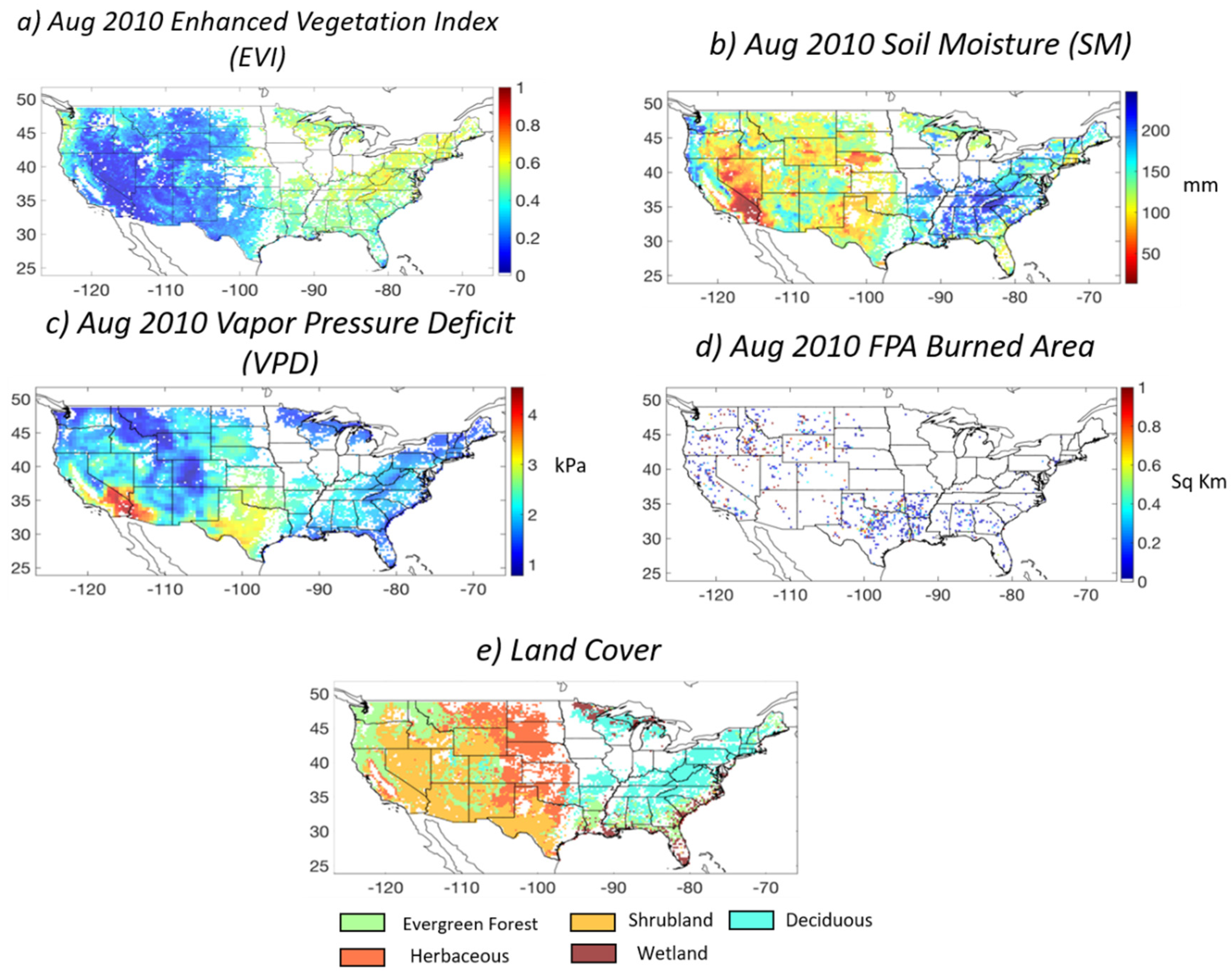
2.1. Datasets
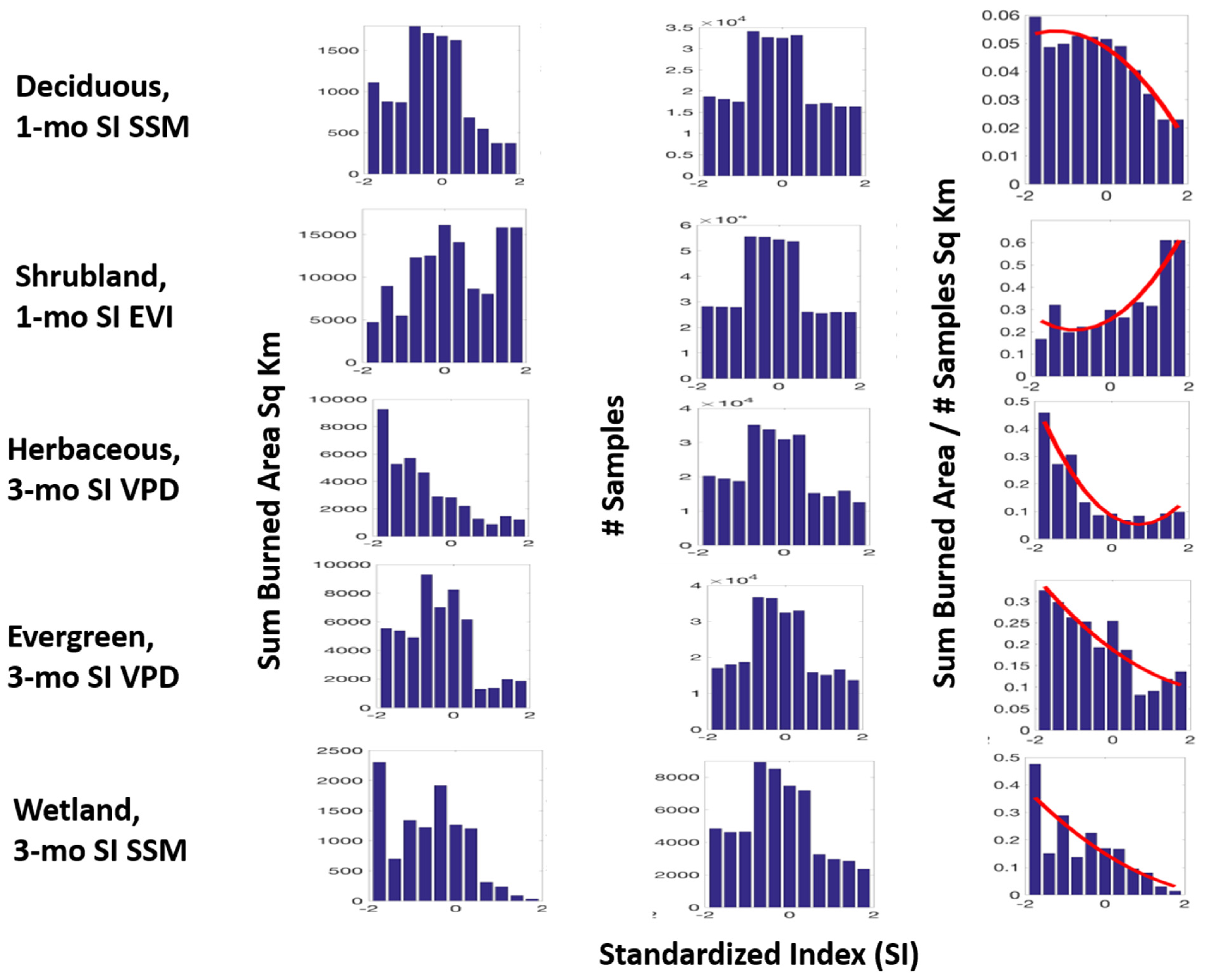
2.2. Converting the Hydrologic and Vegetation Variables to Standardized Indices (SI)
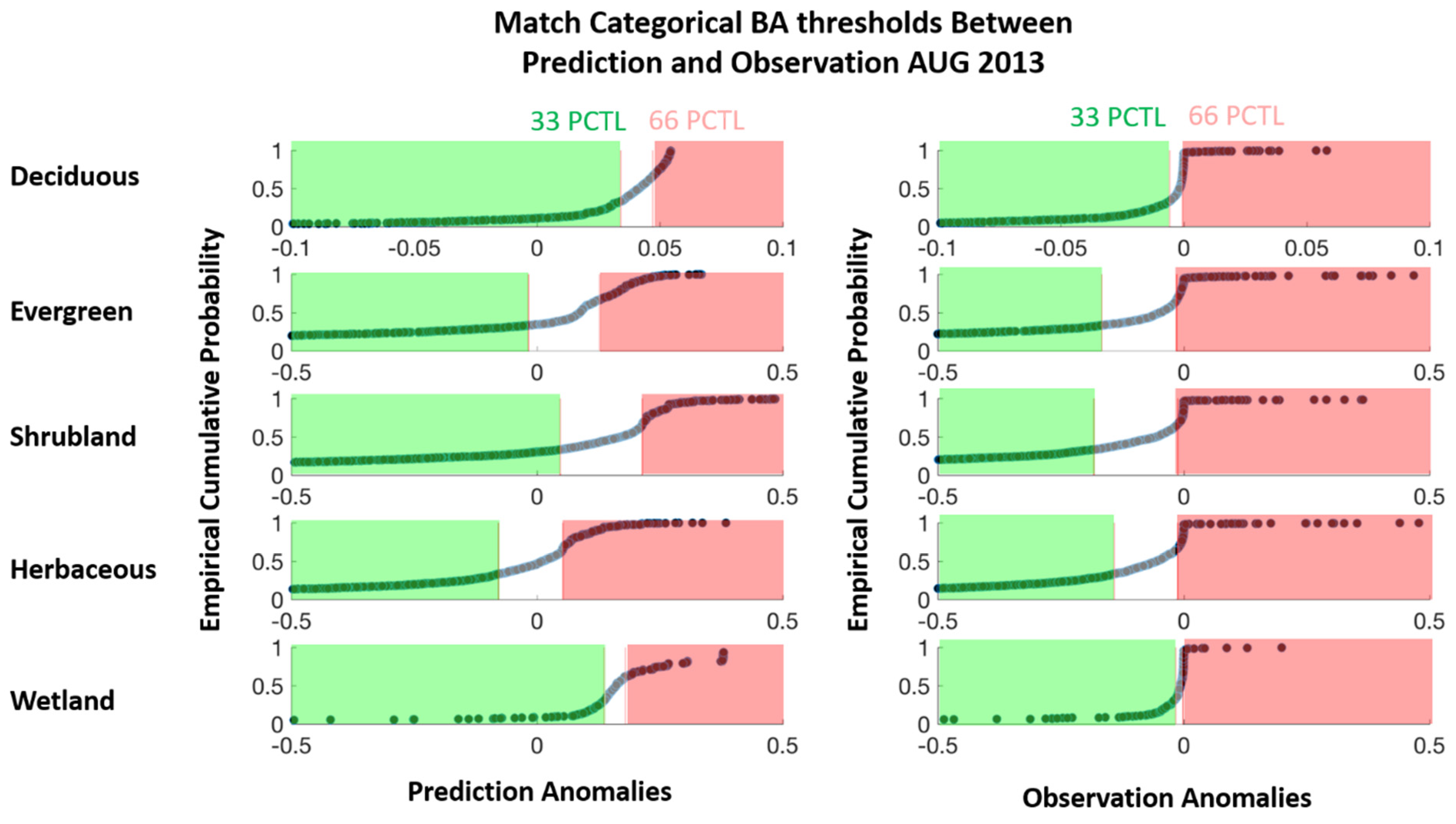
2.3. Model Development
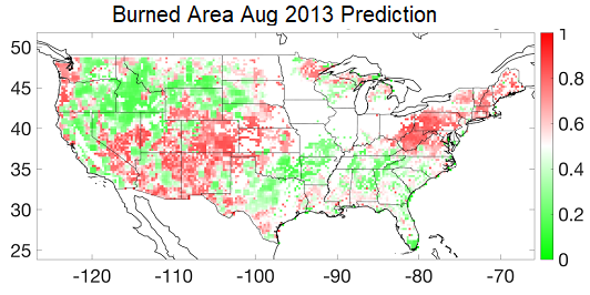
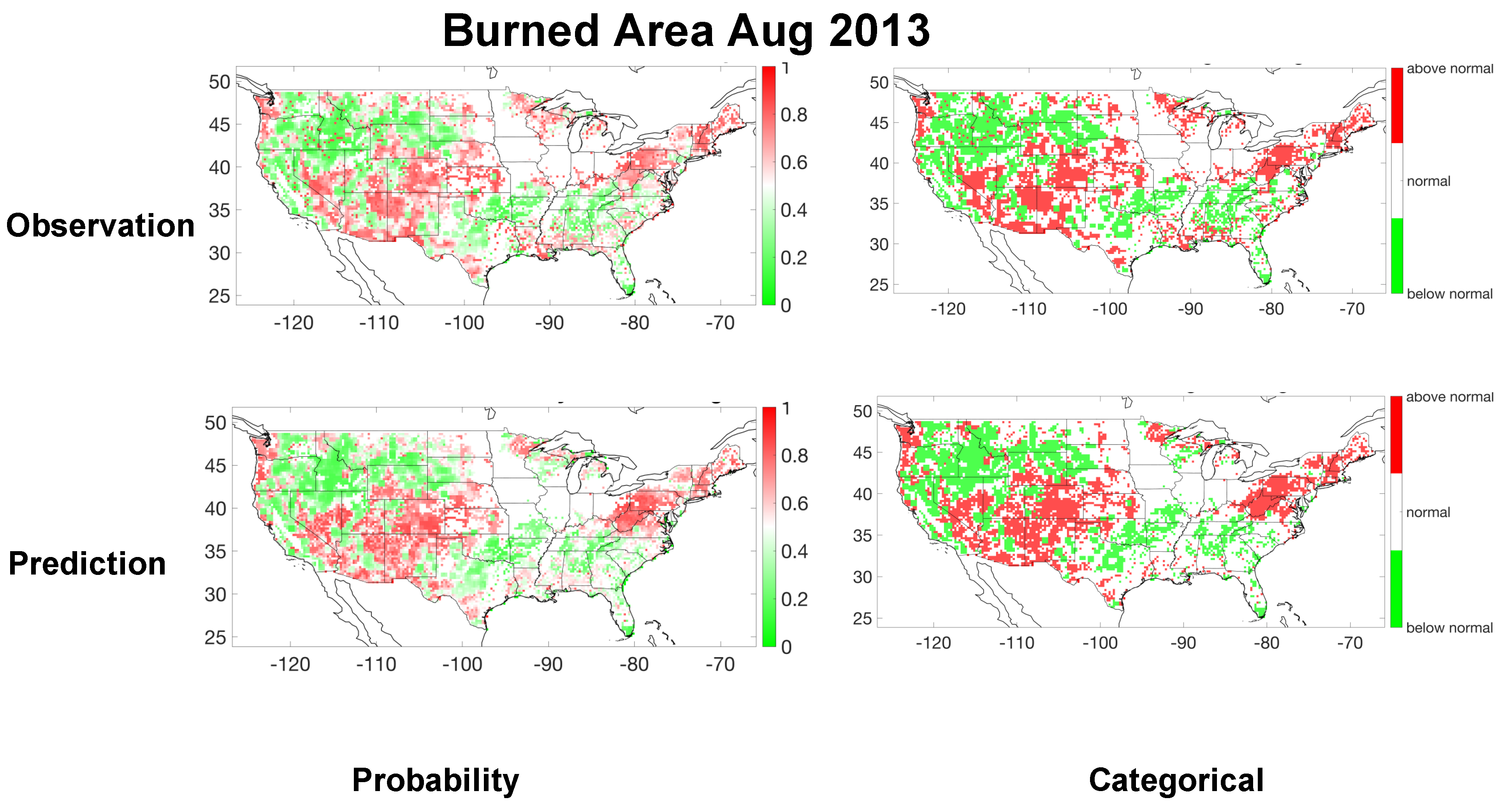
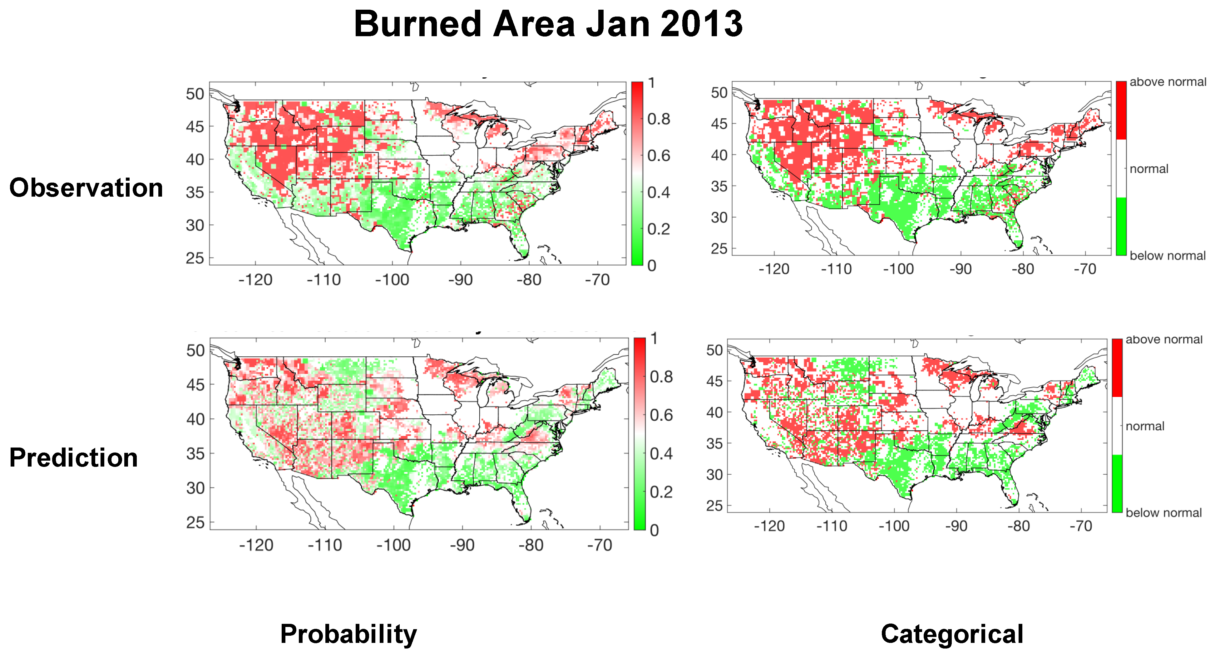
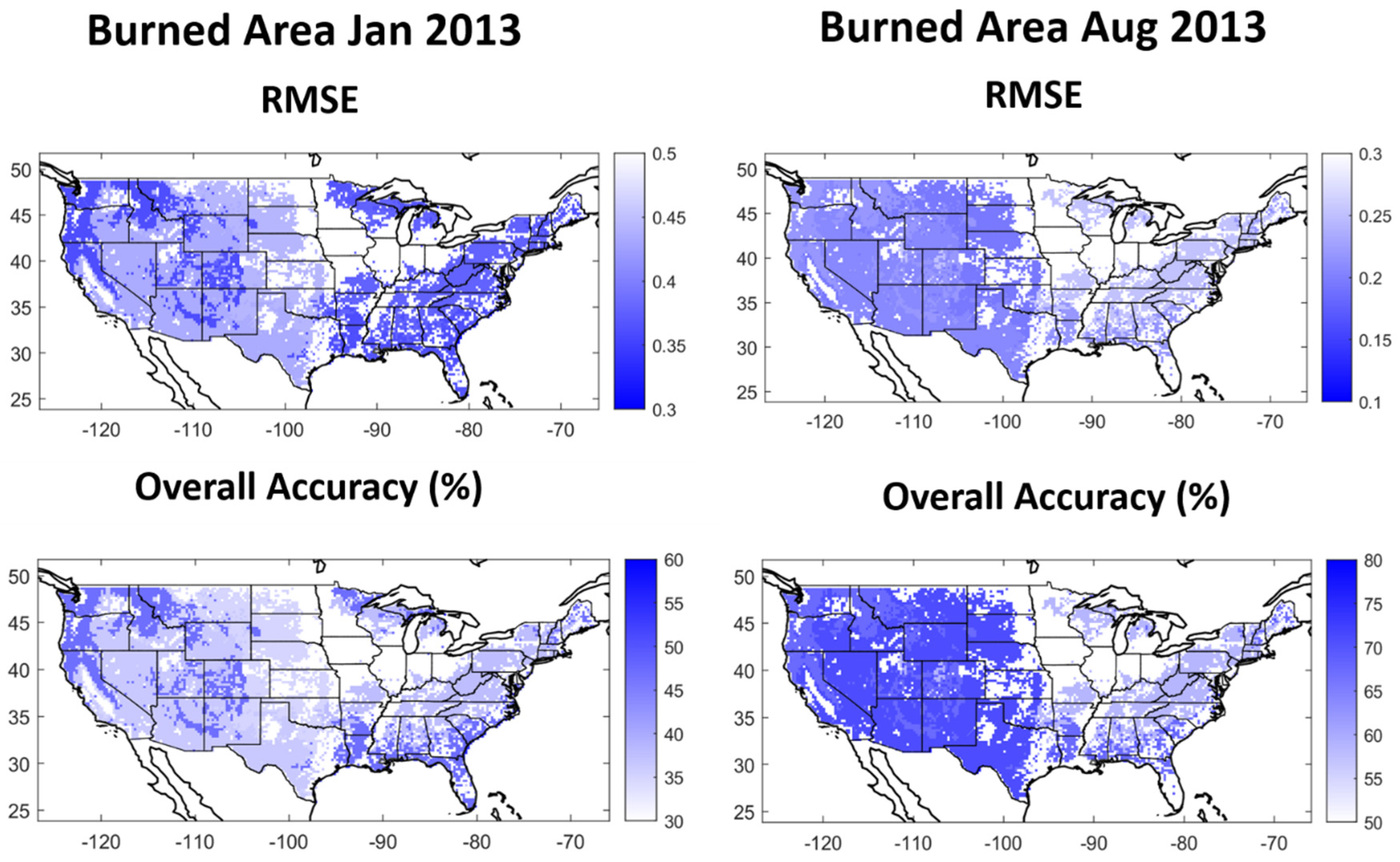
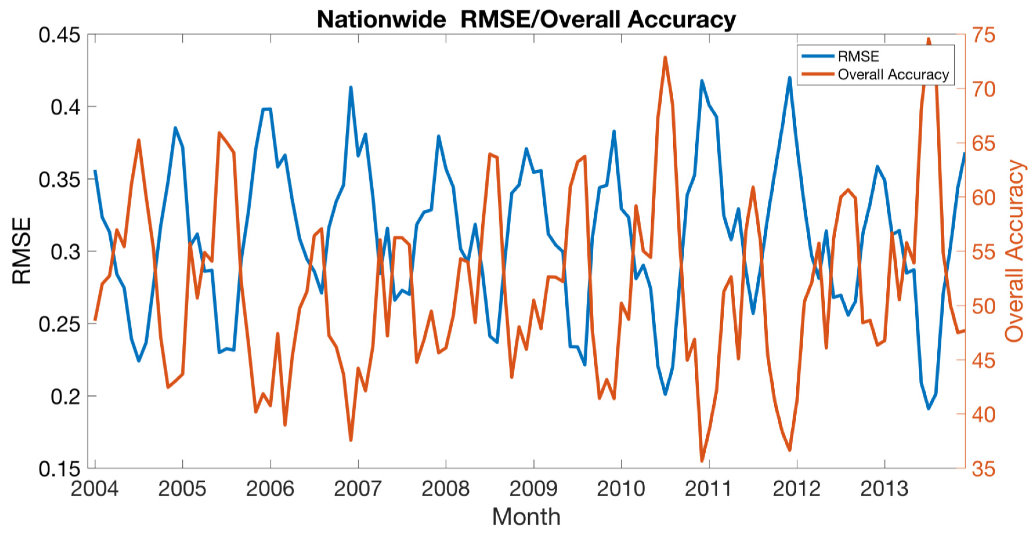
3. Results
4. Discussion
5. Conclusions
Supplementary Materials
Author Contributions
Funding
Acknowledgments
Conflicts of Interest
References
- NIFC. Suppression Costs. Available online: https://www.nifc.gov/fireInfo/fireInfo_documents/SuppCosts.pdf (accessed on 17 October 2018).
- Martell, D.L.; Sun, H. The impact of fire suppression, vegetation, and weather on the area burned by lightning-caused forest fires in Ontario. Can. J. For. Res. 2008, 38, 1547–1563. [Google Scholar] [CrossRef]
- NIFC. Predictive Services. Available online: https://www.predictiveservices.nifc.gov/outlooks/outlooks.htm (accessed on 17 October 2018).
- Bradshaw, L.S.; Deeming, J.E.; Burgan, R.E.; Cohen, J.D. The 1978 National Fire-Danger Rating System: Technical Documentation; U.S. Department of Agriculture, Forest Service, Intermountain Forest and Range Experiment Station: Ogden, UT, USA, 1984. [Google Scholar]
- Abatzoglou, J.T. Development of gridded surface meteorological data for ecological applications and modelling. Int. J. Climatol. 2013, 33, 121–131. [Google Scholar] [CrossRef]
- Holden, Z.A.; Jolly, W.M. Modeling topographic influences on fuel moisture and fire danger in complex terrain to improve wildland fire management decision support. Forest Ecol. Manag. 2011, 262, 2133–2141. [Google Scholar] [CrossRef]
- Easterling, D.R. Global Data Sets for Analysis of Climate Extremes. In Extremes in a Changing Climate; AghaKouchak, A., Easterling, D., Hsu, K., Schubert, S., Sorooshian, S., Eds.; Springer: Dordrecht, The Netherlands, 2013; Volume 65, pp. 347–361. [Google Scholar]
- Abatzoglou, J.T.; Brown, T.J. A comparison of statistical downscaling methods suited for wildfire applications. Int. J. Climatol. 2012, 32, 772–780. [Google Scholar] [CrossRef]
- Bauer, P.; Thorpe, A.; Brunet, G. The quiet revolution of numerical weather prediction. Nature 2015, 525, 47–55. [Google Scholar] [CrossRef]
- Westerling, A.L.; Gershunov, A.; Cayan, D.R.; Barnett, T.P. Long lead statistical forecasts of area burned in western U.S. wildfires by ecosystem province. Int. J. Wildland Fire 2002, 11, 257. [Google Scholar] [CrossRef]
- Beckage, B.; Platt, W.J. Predicting Severe Wildfire Years in the Florida Everglades. Front. Ecol. Environ. 2003, 1, 235. [Google Scholar] [CrossRef]
- Maselli, F. Use of NOAA-AVHRR NDVI images for the estimation of dynamic fire risk in Mediterranean areas. Remote Sens. Environ. 2003, 86, 187–197. [Google Scholar] [CrossRef]
- Hernandez-Leal, P.A.; Arbelo, M.; Gonzalez-Calvo, A. Fire risk assessment using satellite data. Adv. Space Res. 2006, 37, 741–746. [Google Scholar] [CrossRef]
- Preisler, H.K.; Westerling, A.L. Statistical Model for Forecasting Monthly Large Wildfire Events in Western United States. J. Appl. Meteorol. Climatol. 2007, 46, 1020–1030. [Google Scholar] [CrossRef] [Green Version]
- Shabbar, A.; Skinner, W.; Flannigan, M.D. Prediction of Seasonal Forest Fire Severity in Canada from Large-Scale Climate Patterns. J. Appl. Meteorol. Climatol. 2011, 50, 785–799. [Google Scholar] [CrossRef]
- Gudmundsson, L.; Rego, F.C.; Rocha, M.; Seneviratne, S.I. Predicting above normal wildfire activity in southern Europe as a function of meteorological drought. Environ. Res. Lett. 2014, 9, 084008. [Google Scholar] [CrossRef]
- Parks, S.A.; Parisien, M.-A.; Miller, C.; Dobrowski, S.Z. Fire Activity and Severity in the Western US Vary along Proxy Gradients Representing Fuel Amount and Fuel Moisture. PLoS ONE 2014, 9, e99699. [Google Scholar] [CrossRef]
- Seager, R.; Hooks, A.; Williams, A.P.; Cook, B.; Nakamura, J.; Henderson, N. Climatology, Variability, and Trends in the U.S. Vapor Pressure Deficit, an Important Fire-Related Meteorological Quantity. J Appl. Meteorol. Climatol. 2015, 54, 1121–1141. [Google Scholar] [CrossRef]
- Behrangi, A.; Fetzer, E.J.; Granger, S.L. Early detection of drought onset using near surface temperature and humidity observed from space. Int. J. Remote Sens. 2016, 37, 3911–3923. [Google Scholar] [CrossRef]
- Jensen, D.; Reager, J.T.; Zajic, B.; Rousseau, N.; Rodell, M.; Hinkley, E. The sensitivity of US wildfire occurrence to pre-season soil moisture conditions across ecosystems. Environ. Res. Lett. 2018, 13, 014021. [Google Scholar] [CrossRef]
- Farahmand, A.; Stavros, E.N.; Reager, J.T.; Behrangi, A.; Randerson, J.; Quayle, B. Satellite Hydrology Observations as Operational Indicators of Forecasted Fire Danger across the Contiguous United States. 2019; in review. [Google Scholar] [CrossRef]
- Xiao, J.; Zhuang, Q. Drought effects on large fire activity in Canadian and Alaskan forests. Environ. Res. Lett. 2007, 2, 044003. [Google Scholar] [CrossRef]
- MODIS13 Data. Available online: https://lpdaac.usgs.gov/dataset_discovery/modis/modis_products_table/mod13c2_v006 (accessed on 20 November 2018).
- Huete, A.; Didan, K.; Miura, T.; Rodriguez, E.P.; Gao, X.; Ferreira, L.G. Overview of the radiometric and biophysical performance of the MODIS vegetation indices. Remote Sens. Environ. 2002, 83, 195–213. [Google Scholar] [CrossRef]
- Rouse, J.W.; Haas, R.H.; Schell, J.A.; Deering, D.W. Monitoring Vegetation Systems in the Great Plains with ERTS. In Proceedings of the Third Earth Resources Technology Satellite- 1 Symposium, Washington, DC, USA, 1 January 1974; NASA SP-351. Volume 1, pp. 309–317. [Google Scholar]
- Schnur, M.T.; Xie, H.; Wang, X. Estimating root zone soil moisture at distant sites using MODIS NDVI and EVI in a semi-arid region of southwestern USA. Ecol. Inform. 2010, 5, 400–409. [Google Scholar] [CrossRef]
- Aumann, H.H.; Chahine, M.T.; Gautier, C.; Goldberg, M.D.; Kalnay, E.; McMillin, L.M.; Revercomb, H.; Rosenkranz, P.W.; Smith, W.L.; Staelin, D.H.; et al. AIRS/AMSU/HSB on the aqua mission: Design, science objectives, data products, and processing systems. IEEE Trans. Geosci. Remote Sens. 2003, 41, 253–264. [Google Scholar] [CrossRef] [Green Version]
- Goldberg, M.D.; Qu, Y.; McMillin, L.M.; Wolf, M.; Zhou, L.; Divakarla, M. AIRS near-real-time products and algorithms in support of operational numerical weather prediction. IEEE Trans. Geosci. Remote Sens. 2003, 41, 379–389. [Google Scholar] [CrossRef]
- Zaitchik, B.F.; Rodell, M.; Reichle, R.H. Assimilation of GRACE Terrestrial Water Storage Data into a Land Surface Model: Results for the Mississippi River Basin. J. Hydrometeorol. 2008, 9, 535–548. [Google Scholar] [CrossRef]
- Houborg, R.; Rodell, M.; Li, B.; Reichle, R.; Zaitchik, B.F. Drought indicators based on model-assimilated Gravity Recovery and Climate Experiment (GRACE) terrestrial water storage observations: GRACE-BASED DROUGHT INDICATORS. Water Resour. Res. 2012, 48. [Google Scholar] [CrossRef] [Green Version]
- Reager, J.; Thomas, A.; Sproles, E.; Rodell, M.; Beaudoing, H.; Li, B.; Famiglietti, J. Assimilation of GRACE Terrestrial Water Storage Observations into a Land Surface Model for the Assessment of Regional Flood Potential. Remote Sens. 2015, 7, 14663–14679. [Google Scholar] [CrossRef] [Green Version]
- Tapley, B.D.; Bettadpur, S.; Watkins, M.; Reigber, C. The gravity recovery and climate experiment: Mission overview and early results: GRACE MISSION OVERVIEW AND EARLY RESULTS. Geophys. Res. Lett. 2004, 31. [Google Scholar] [CrossRef] [Green Version]
- Short, K.C. Spatial Wildfire Occurrence Data for the United States, 1992–2013 [FPA_FOD_20150523], 3rd ed.; Forest Service Research Data Archive: Fort Collins, CO, USA, 2015. [Google Scholar] [CrossRef]
- Short, K.C. A spatial database of wildfires in the United States, 1992–2011. Earth Syst. Sci. Data 2014, 6, 1–27. [Google Scholar] [CrossRef] [Green Version]
- Homer, C.; Dewitz, J.; Yang, L.; Jin, S.; Danielson, P.; Xian, G.; Coulston, J.; Herold, N.; Wickham, J.; Megown, K. Completion of the 2011 National Land Cover Database for the conterminous United States–representing a decade of land cover change information. Photogramm. Eng. Remote Sens. 2015, 81, 345–354. [Google Scholar]
- Littell, J.S.; McKenzie, D.; Peterson, D.L.; Westerling, A.L. Climate and wildfire area burned in western U.S. ecoprovinces, 1916–2003. Ecol. Appl. 2009, 19, 1003–1021. [Google Scholar] [CrossRef]
- Farahmand, A.; AghaKouchak, A. A generalized framework for deriving nonparametric standardized drought indicators. Adv. Water Resour 2015, 76, 140–145. [Google Scholar] [CrossRef]
- Stavros, E.N.; Abatzoglou, J.; Larkin, N.K.; McKenzie, D.; Steel, E.A. Climate and very large wildland fires in the contiguous western USA. Int. J. Wildland Fire 2014, 23, 899. [Google Scholar] [CrossRef]
- Congalton, R.G. A review of assessing the accuracy of classifications of remotely sensed data. Remote Sens. Environ. 1991, 37, 35–46. [Google Scholar] [CrossRef]
- Barbero, R.; Abatzoglou, J.T.; Steel, E.A.; K Larkin, N. Modeling very large-fire occurrences over the continental United States from weather and climate forcing. Environ. Res. Lett. 2014, 9, 124009. [Google Scholar] [CrossRef]
- Morgan, P.; Hardy, C.C.; Swetnam, T.W.; Rollins, M.G.; Long, D.G. Mapping fire regimes across time and space: Understanding coarse and fine-scale fire patterns. Int. J. Wildland Fire 2001, 10, 329. [Google Scholar] [CrossRef] [Green Version]
- Jin, Y.; Randerson, J.T.; Faivre, N.; Capps, S.; Hall, A.; Goulden, M.L. Contrasting controls on wildland fires in Southern California during periods with and without Santa Ana winds: Controls on Southern California fires. J. Geophys. Res. Biogeosci. 2014, 119, 432–450. [Google Scholar] [CrossRef] [Green Version]
- Agee, J.K. Fire Ecology of Pacific Northwest Forests; Island Press: Washington, DC, USA, 1996. [Google Scholar]
- Sugihara, N.G.; Van Wagtendonk, J.W.; Fites-Kaufman, J. Fire as an Ecological Process. In Fire in California’s Ecosystems; University of California Press: Berkeley, CA, USA, 2006; pp. 38–74. [Google Scholar]
- Aids to Determining Fuel Models for Estimating Fire Behavior. Available online: https://www.fs.usda.gov/treesearch/pubs/6447 (accessed on 1 April 2020).
- Standard Fire Behavior Fuel Models: A Comprehensive Set for Use with Rothermel’s Surface Fire Spread Model. Available online: https://www.fs.usda.gov/treesearch/pubs/9521 (accessed on 1 April 2020).
- Pederson, N.; Dyer, J.M.; McEwan, R.W.; Hessl, A.E.; Mock, C.J.; Orwig, D.A.; Rieder, H.E.; Cook, B.I. The legacy of episodic climatic events in shaping temperate, broadleaf forests. Ecol. Monogr. 2014, 84, 599–620. [Google Scholar] [CrossRef]
- Mitchell, R.J.; Liu, Y.; O’Brien, J.J.; Elliott, K.J.; Starr, G.; Miniat, C.F.; Hiers, J.K. Future climate and fire interactions in the southeastern region of the United States. Forest Ecol. Manag. 2014, 327, 316–326. [Google Scholar] [CrossRef]
- Littell, J.S.; Peterson, D.L.; Riley, K.L.; Liu, Y.; Luce, C.H. A review of the relationships between drought and forest fire in the United States. Glob. Chang. Biol. 2016, 22, 2353–2369. [Google Scholar] [CrossRef]
- Jolly, W.M.; Cochrane, M.A.; Freeborn, P.H.; Holden, Z.A.; Brown, T.J.; Williamson, G.J.; Bowman, D.M.J.S. Climate-induced variations in global wildfire danger from 1979 to 2013. Nat. Commun. 2015, 6, 1–11. [Google Scholar] [CrossRef]
- Jaffe, D.; Hafner, W.; Chand, D.; Westerling, A.; Spracklen, D. Interannual Variations in PM2.5 due to Wildfires in the Western United States. Environ. Sci. Technol. 2008, 42, 2812–2818. [Google Scholar] [CrossRef]
- Chaparro, D.; Piles, M.; Vall-llossera, M.; Camps, A. Surface moisture and temperature trends anticipate drought conditions linked to wildfire activity in the Iberian Peninsula. Eur. J. Remote. Sens. 2016, 49, 955–971. [Google Scholar] [CrossRef] [Green Version]
- Balch, J.K.; Bradley, B.A.; Abatzoglou, J.T.; Nagy, R.C.; Fusco, E.J.; Mahood, A.L. Human-started wildfires expand the fire niche across the United States. In Proceedings of the National Academy of Sciences, Stanford, CA, USA, 20 October 2016. [Google Scholar]
- Chang, Y.; Zhu, Z.; Bu, R.; Chen, H.; Feng, Y.; Li, Y.; Hu, Y.; Wang, Z. Predicting fire occurrence patterns with logistic regression in Heilongjiang Province, China. Landscape Ecol. 2013, 28, 1989–2004. [Google Scholar] [CrossRef]
- Costafreda-Aumedes, S.; Comas, C.; Vega-Garcia, C. Human-caused fire occurrence modelling in perspective: A review. Int. J. Wildland Fire 2017, 26, 983. [Google Scholar] [CrossRef]
- Kuhnert, P.M.; Martin, T.G.; Griffiths, S.P. A guide to eliciting and using expert knowledge in Bayesian ecological models: Expert elicitation and use in Bayesian models. Ecol. Lett. 2010, 13, 900–914. [Google Scholar] [CrossRef] [PubMed]
- Drescher, M.; Perera, A.H.; Johnson, C.J.; Buse, L.J.; Drew, C.A.; Burgman, M.A. Toward rigorous use of expert knowledge in ecological research. Ecosphere 2013, 4, 1–26. [Google Scholar] [CrossRef]


| Land Cover Type | RMSE Mean | RMSE SD | Overall Accuracy Mean (%) | Error Underestimate (%) | Error Overestimate (%) | Overall Accuracy SD |
|---|---|---|---|---|---|---|
| Deciduous | 0.28 | 0.05 | 54.5 | 20 | 25.5 | 9.9 |
| Evergreen | 0.31 | 0.08 | 52.5 | 24.2 | 23.3 | 14 |
| Shrubland | 0.32 | 0.07 | 51.7 | 25.3 | 23 | 13.8 |
| Herbaceous | 0.3 | 0.07 | 54.2 | 23.2 | 22.6 | 11.75 |
| Wetland | 0.35 | 0.05 | 45.5 | 26.5 | 28 | 9.75 |
| CONUS | 0.31 | 0.05 | 52.8 | 23.6 | 23.6 | 8 |
© 2020 by the authors. Licensee MDPI, Basel, Switzerland. This article is an open access article distributed under the terms and conditions of the Creative Commons Attribution (CC BY) license (http://creativecommons.org/licenses/by/4.0/).
Share and Cite
Farahmand, A.; Stavros, E.N.; Reager, J.T.; Behrangi, A. Introducing Spatially Distributed Fire Danger from Earth Observations (FDEO) Using Satellite-Based Data in the Contiguous United States. Remote Sens. 2020, 12, 1252. https://doi.org/10.3390/rs12081252
Farahmand A, Stavros EN, Reager JT, Behrangi A. Introducing Spatially Distributed Fire Danger from Earth Observations (FDEO) Using Satellite-Based Data in the Contiguous United States. Remote Sensing. 2020; 12(8):1252. https://doi.org/10.3390/rs12081252
Chicago/Turabian StyleFarahmand, Alireza, E. Natasha Stavros, John T. Reager, and Ali Behrangi. 2020. "Introducing Spatially Distributed Fire Danger from Earth Observations (FDEO) Using Satellite-Based Data in the Contiguous United States" Remote Sensing 12, no. 8: 1252. https://doi.org/10.3390/rs12081252