Article

Vessel Tracking Using Bistatic Compact HFSWR

1
College of Oceanography and Space Informatics, China University of Petroleum (East China), Qingdao 266580, China
2
Faculty of Engineering and Applied Science, Memorial University of Newfoundland, St. John’s, NL A1B 3X5, Canada
3
Laboratory of Marine Physics and Remote Sensing, First Institute of Oceanography, Ministry of Natural Resources, Qingdao 266061, China
*
Author to whom correspondence should be addressed.
Remote Sens. 2020, 12(8), 1266; https://doi.org/10.3390/rs12081266
Submission received: 21 March 2020 / Revised: 14 April 2020 / Accepted: 15 April 2020 / Published: 16 April 2020
(This article belongs to the Special Issue Bistatic HF Radar)

Abstract

:
Bistatic and multi-static high-frequency surface wave radar (HFSWR) is becoming a prospective development trend for sea surface surveillance due to its potential in extending the coverage area, improving the detection accuracy, etc. In this paper, the vessel detection and tracking performance of a newly developed bistatic compact HFSWR system whose transmitting and receiving antennas are not co-located was investigated. Firstly, the representation of the target range and Doppler velocity concerning a bistatic HFSWR was derived and compared with that of a monostatic system. Next, taking the characteristics of target kinematic parameters into account, a target tracking method applicable to a bistatic HFSWR is proposed. The simultaneous target tracking results from both monostatic and bistatic HFSWR field data are presented and compared. The experimental results demonstrate the good performance in target tracking of the bistatic HFSWR and also show that an HFSWR system combining monostatic and bistatic modes has the potential to enhance the target track continuity and improve the detection accuracy.

Graphical Abstract

1. Introduction

High-frequency surface wave radar (HFSWR) operated in the 3–30 MHz frequency band has been recognized as an important maritime surveillance tool [1] for both sea state monitoring [2] and hard target detection [3] due to its superiority of over-the-horizon coverage, all-weather and continuous surveillance, high time resolution, low-cost, etc. Existing HFSWRs for hard target detection are monostatic with the transmitter and receiver being co-located. Some HFSWRs employ a linear receiving array with a large aperture size and high transmitting power to achieve high azimuth resolution and long detection range. e.g., the SWR-503 system developed in Canada uses a receiving array with an aperture size of 660 m and a transmitting power of 30 kW. Such a radar system usually requires a large coastline area, which makes it difficult for site selection, system deployment, and maintenance, and thus limits its operational applications. Therefore, system miniaturization has become a new development trend [4]. So far, two kinds of compact HFSWR systems with small aperture size have been developed. One utilizes crossed-loop/monopole antennas, such as the SeaSonde system developed by CODAR [5,6], the OSMAR system developed by Wuhan University [7], etc., while the other still uses phased array antenna but with less antenna array elements (e.g., 3–8 elements), e.g., the WERA-S system developed by Helzel MessTechnik [8], the Compact Over-the-horizon Radar for Maritime Surveillance (CORMS) system developed by our team [9,10,11], etc.
Compared with an HFSWR system that has large aperture size, a small-aperture compact system has the advantages of flexible deployment and maintenance. It can be installed on a small island, or even on a large ship [12], thus increasing the detection flexibility and extending coverage area. However, it should be noted that the direction of arrival estimation performance degrades due to the reduced number of antenna elements. The resultant poor azimuth estimation accuracy may lead to large target positioning errors. In addition, the lower transmitting power and clutter interference, such as the sea clutter, ionospheric clutter, etc., make target detection more challenging.
To improve the target detection performance of compact HFSWRs, on one hand, super-resolution direction-finding methods, such as MUSIC [13], were proposed to improve the azimuth estimation accuracy. On the other hand, distributed multi-radar systems, such as bistatic and multi-static radar [14], MIMO radar [15], etc., were designed to simultaneously monitor the targets in a common area of interest from different perspectives. Also, bistatic or multi-static configuration makes the influence of sea clutter, ionosphere clutter, etc., diverse from different sites. The complementary information obtained from different radars can be associated and fused to produce more precise results. However, the distributed radar systems with multiple radars are inherently more complex and hence tend to be more expensive. Multi-static radar offers a way to obtain good target detection performance but requires extensive research, especially advanced signal processing techniques. Among distributed radar systems, the combination of one monostatic radar and one bistatic radar with a common transmitting station and two separate receiving stations, i.e., T/R-R radar, is a typical configuration that offers a tradeoff between system performance and complexity. In this paper, the target detection and tracking performance of a T/R-R bistatic compact HFSWR system is investigated. It is worth noting that although the T/R-R configuration brings several advantages in target detection, the problems caused by the compact HFSWR system itself, such as low detection precision for both range and azimuth, are inherent.
Although bistatic system is not a new concept, very few bistatic HFSWRs have been developed and limited experiments have been reported. Theoretical studies on bistatic HFSWR have been carried out extensively. For example, various issues related to bistatic HFSWR, such as system configuration, site selection, spectral characteristics, detection performance, etc., were analyzed in [16,17,18]. Clutter models were established in [19] and analyzed in [20], and interference suppression methods were proposed in [21]. Different ocean surface radar cross section models of bistatic HFSWR were derived and analyzed in [22,23,24,25,26,27,28]. However, experimental work is relatively limited. So far, bistatic HFSWRs have been utilized for surface current mapping [29,30,31], directional ocean spectrum measurement [32], and wind direction measurement [33] over a very short period. Existing research related to bistatic HFSWR mainly focuses on system design and performance analysis, scattering mechanism investigation, clutter suppression, and sea state mapping applications. Most of the research work lies in theoretical analysis and numerical simulation. Compared with the numerous multi-target tracking (MTT) algorithms developed for monostatic HFSWRs [34,35,36], target detection and tracking using bistatic HFSWR have been much less explored [37], especially with field data.
The primary objective of this paper was to investigate the characteristics of target detection with a bistatic HFSWR and develop an applicable target tracking method accordingly. The field data collected by a newly developed T/R-R compact HFSWR were used to validate the correctness of the derived results and verify the performance of the proposed tracking method. Besides, comparisons were made between the tracking results of monostatic and bistatic HFSWR. The remainder of this paper is organized as follows. Section 2 describes the characteristics of target representation for a bistatic HFSWR, followed by a detailed description of an applicable target tracking method. In Section 3, the experimental results are presented and analyzed. Discussions are provided in Section 4 and conclusions are drawn in Section 5.

2. Target Detection and Tracking with a Bistatic Compact HFSWR

The combined monostatic and bistatic compact HFSWR system, abbreviated as a T/R-R compact HFSWR system in the following description, employs a common transmitter and two receivers. The co-located transmitter and receiver constitute a monostatic radar, while the bistatic radar is composed of the shared transmitter and the other receiver deployed at a considerable distance away from the transmitter. As target detection is the basis of target tracking, the target representation method for a bistatic HFSWR is discussed first.

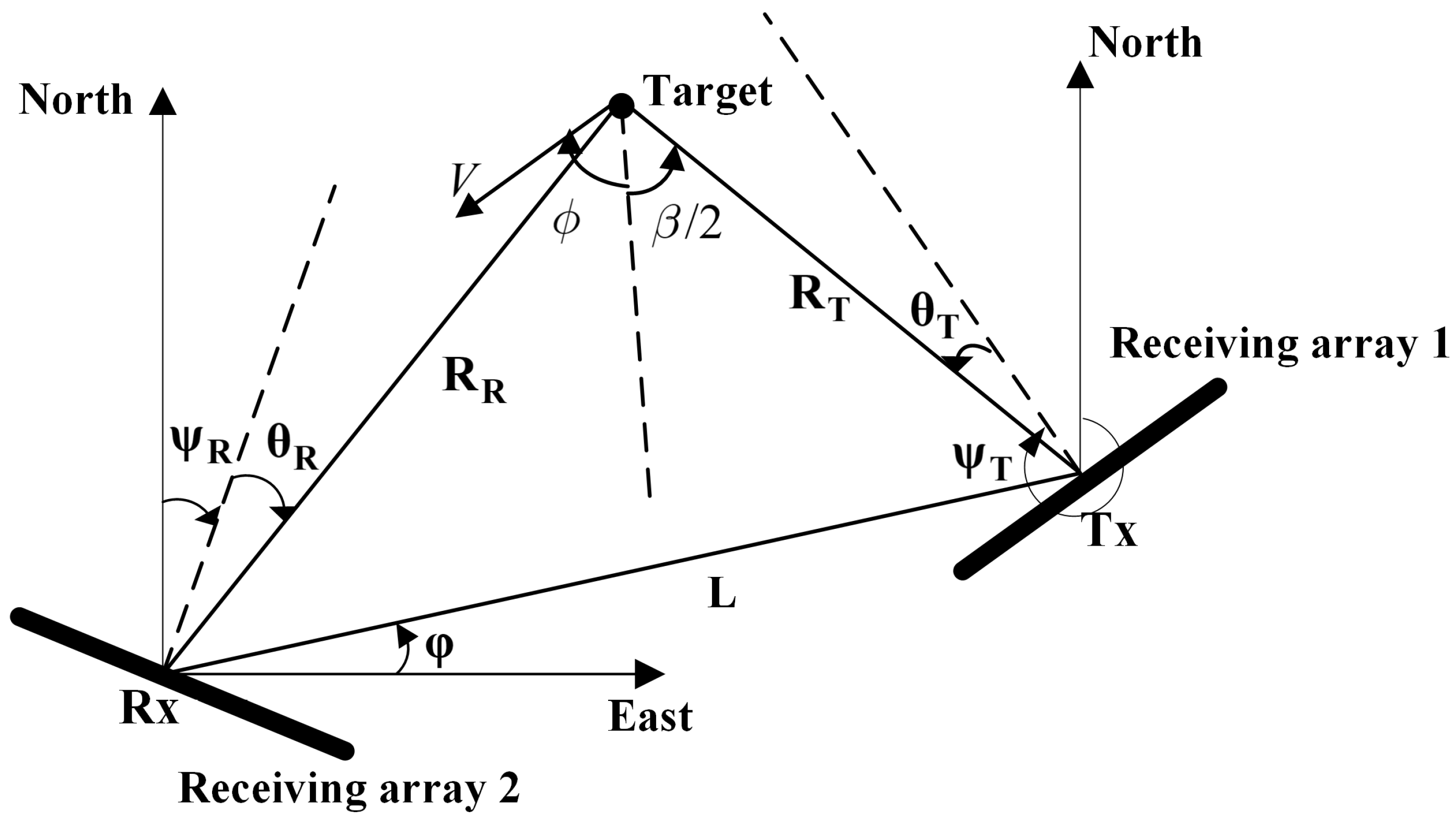
2.1. Target Representation with a Bistatic Compact HFSWR

Compared with a monostatic HFSWR, a bistatic HFSWR represents a target differently due to different geometry. The target detection geometry of a T/R-R HFSWR system, defined by the position of a transmitter (Tx), a receiver (Rx), and a target using a two-dimensional north-referenced coordinate system, is illustrated in Figure 1.
In Figure 1, the transmitter and receiving array 1 are deployed at the transmitting station (Tx), while receiving array 2 is deployed at the receiving station (Rx). The transmitter serves the two receiving arrays simultaneously. The distance L between the transmitter and receiver is called the bistatic range or simply the baseline. φ denotes the angle between the baseline and East direction. Denote ψ T and ψ R , respectively, as the radar look directions of receiving array 1 and receiving array 2 with respect to true North. β is the bistatic angle. For a moving target with a velocity of magnitude V and aspect angle ϕ referenced to the bistatic bisector, the monostatic radar represents a target as a plot with a state vector [ R T θ T v d T ] in a polar coordinate, with R T , θ T , v d T being the range, azimuth, and Doppler velocity measured at the transmitting station. Similarly, the bistatic radar represents a target as a plot with a state vector [ R R θ R v d R ] , with R R , θ R , v d R being the range, azimuth, and Doppler velocity calculated at the receiving station. As the estimation methods of R T , θ T , and v d T for monostatic HFSWR has been investigated [11], only the estimation methods of R R , θ R , and v d R for the bistatic HFSWR are discussed here.
Like the monostatic case, a target azimuth θ R is also estimated using the digital beaming forming (DBF) method for a bistatic HFSWR with a linear phased array as its receiving antenna. θ R takes negative values on the left side of the radar boresight, and positive values on the other side. However, the estimation methods for range and Doppler velocity are different from those used in a monostatic HFSWR. Firstly, the distance directly measured by a bistatic radar is the sum of R T and R R , the total transmitter-to-target-to-receiver scattering path, instead of R R . Target positions with the same range sum, i.e., the isorange contour, form an ellipse with foci at the transmitter and receiver sites. The bisector of the bistatic angle β is orthogonal to the tangent of the ellipse and passes through a target position. Thus, a target position can be determined by its range sum and estimated azimuth θ R . As can be seen from Figure 1, either ( R R , θ R ) or ( R T , θ T ) can be exclusively used for target location representation. For monostatic HFSWR, R R = R T , and θ R = θ T , thus its target tracking methods cannot be directly applied to the bistatic case. Considering that the target azimuth θ R is directly measured by the receiving antenna array 2 with respect to its normal direction, ( R R , θ R ) instead of ( R T , θ T ) is chosen to specify the target position for bistatic HFSWR. i.e., R R is used to represent the target range and is derived as follows.
According to the bistatic triangle (i.e., the transmitter–target–receiver triangle shown in Figure 1) relationship, the following relation can be obtained:
R T 2 = R R 2 + L 2 2 R R L cos ( π 2 ψ R θ R φ ) .
Denote R = R T + R R , θ = ψ R + θ R + φ , then R R can be calculated as
R R = R 2 L 2 2 ( R L sin θ ) .
Once the radar configuration is set, ψ R , L, and φ are known. R and θ R can be determined from the data collected by the linear receiving array 2, then R R can be calculated by Equation (2). The calculated R R and the estimated θ R can also specify the location of the target. However, unlike the monostatic case, the calculated range R R is a function of the estimated target azimuth θ R . The coarse azimuth resolution of a compact HFSWR leads to large estimation errors in R R , which brings greater challenges for target detection and tracking with bistatic compact HFSWR.
Another difference from a monostatic radar is the estimated Doppler velocity. The Doppler velocity measured by a monostatic radar is along the radial direction in the polar coordinate system with origin at the radar site, while the Doppler velocity estimated from a range-Doppler spectrum of a bistatic radar is along the direction of the bistatic bisector. It is the resultant velocity combining the Doppler velocities measured from the transmitting and receiving stations. The estimated elliptical Doppler velocity can be calculated as
V d R = d R d t = d R T d t + d R R d t = V cos ( ϕ + β 2 ) + V cos ( ϕ β 2 ) = 2 V cos ϕ cos ( β 2 ) .
It can be concluded that the magnitude of the bistatic Doppler velocity is related to the bistatic angle and is never greater than that of a monostatic radar. In practice, the measured Doppler velocity v d R is obtained from the Doppler shift f d extracted from a bistatic range-Doppler spectrum by
v d R = ( f d · c ) / f o ,
where f d denotes the radar operating frequency, c is the light speed.
Sea surface target detection using compact HFSWR is typically affected by either ocean clutter or ionospheric clutter, which can mask the returns from targets at their corresponding Doppler points and make them undetectable. In addition to parameter representations of a target discussed above, the first-order sea clutter should also be considered for target detection with a bistatic HFSWR. Without the effect of surface current, for stationary transmitting and receiving antennas, the Doppler shift of the first-order sea clutter for a bistatic HFSWR [22] can be written as
f b = ± g cos ( β / 2 ) π λ ,
where λ denotes the radar wavelength, g is the gravity acceleration. Equation (5) indicates that the first-order Bragg shift of a bistatic HFSWR is a function of the bistatic angle β . It is less than that of a monostatic HFSWR, which can be expressed as f b = ± g π λ . For a compact HFSWR, its detection range is limited due to the lower transmitting power; and its beamwidth is wider due to the smaller aperture size. Thus, the bistatic angle β always takes a relatively larger value leading to a spread first-order spectrum, which may mask the targets and increases the challenge for target detection.

2.2. Target Tracking with a Bistatic Compact HFSWR

Once the plot data sequence is consecutively obtained with each plot being denoted by a measured state vector [ R R m θ R m v d R m ] , a multi-target tracking method is required to produce target tracks. The proposed MTT algorithm was modified from the method presented in [11], which is developed from Converted Measurement Kalman Filter (CMKF) and a data association method based on minimal cost. In this method, data association, state prediction, and state estimation are three key steps, where data association is performed in the polar coordinate with the receiving radar site as its origin, while state prediction and estimation are implemented in a Cartesian coordinate.
The state prediction and estimation using the CMKF method are implemented by a linear Kalman filter, which is based on a specific dynamic model and an observation model. Taking the motion characteristic of large vessels into consideration, the target dynamic model is defined in a Cartesian coordinate as
x k = F x k 1 + ω k ,
where x k = [ x k , v x k , y k , v y k ] T is the true state vector at time k in the Cartesian coordinate with the boresight of the receiving array 2 as its x-axis, the direction perpendicular to the radar boresight as the y-axis. x k and y k denote the true target position components, v x k and v y k denote the corresponding true velocity components along x and y directions. [ · ] T denotes the transpose operator. ω k represents the Gaussian process noise with zero mean and covariance matrix Q k . F is the state transition matrix defined as
F = 1 T 0 0 0 1 0 0 0 0 1 T 0 0 0 1 ,
where T denotes the sampling time.
The observation model is also defined in the Cartesian coordinate as
z k = H x k + v k ,
where z k = [ x ˜ k , v ˜ x k , y ˜ k , v ˜ y k ] T is a measured state vector at time k, x ˜ k and y ˜ k denote the measured target position components, v ˜ x k and v ˜ y k are the corresponding measured velocity components along x and y directions, respectively. v k represents measurement noise following Gaussian distribution with zero mean and covariance matrix R k . H is the measurement matrix and it is an identity matrix here.
The difference in the tracking procedure between a monostatic and a bistatic HFSWR lies in that the measured state vector [ R R m θ R m v d R m ] instead of [ R T m θ T m v d T m ] is used. On one hand, the accuracy of R R m , which is related to the coarsely estimated azimuth as shown in Equation (2), is lower than R T m . On the other hand, the elliptical Doppler velocity v d R m that is along the bistatic bisector is used here, and it is assumed that the elliptical Doppler velocity of a target does not change much during a coherent integration time. Thus, the data association procedure is modified by using different target parameters, validation gate thresholds, and association weights. Based on the above analysis, the proposed target tracking procedure for a bistatic compact HFSWR, including three parallel sub-procedures, i.e., track initiation, track maintenance, and track termination, is summarized as follows.
A. Track initiation
Tracks are initiated by the logic method with the M-of-N rule [38]. If a track is successfully initiated with more than M plots connected in the most recent N frames, it will go to the track maintenance procedure; otherwise, it will be dropped.
B. Track maintenance
Step 1: State prediction. For each initiated or maintained track with n plots, denote x ^ k 1 = [ x ^ k 1 , v ^ x k 1 , y ^ k 1 , v ^ y k 1 ] T as its previous plot at time k 1 , its predicted state x ^ k | k 1 = [ x ^ k | k 1 , v ^ x k | k 1 , y ^ k | k 1 , v ^ y k | k 1 ] T at time k is obtained by x ^ k | k 1 = F x ^ k 1 . Meanwhile, the corresponding state prediction covariance P k | k 1 is calculated according to P k | k 1 = F P k 1 F + Q k .
Step 2: Coordinate conversion. The predicted state x ^ k | k 1 is converted from Cartesian coordinate to polar coordinate by
R R k p = x ^ k | k 1 2 + y ^ k | k 1 2 , θ R k p = arctan ( y ^ k | k 1 x ^ k | k 1 ) , v d R k p = x ^ k | k 1 v ^ x k | k 1 + y ^ k | k 1 v ^ y k | k 1 x ^ k | k 1 2 + y ^ k | k 1 2 .
Step 3: Data association. The data association method based on the minimal cost in Equation (9) is utilized to find the most likely measurements [ R R k m θ R k m v d R k m ] at time k within a predefined validation gate. The minimal cost criterion is defined by
c o s t = 1 c o s t v d + c o s t R + c o s t θ ,
where c o s t v d , c o s t R , c o s t θ represent the association cost of Doppler velocity, range, and azimuth, respectively, which are defined as
c o s t v d = W v d exp ( v d R k m v d R k p 2 / σ v d 2 ) , c o s t R = W R exp ( R R k m R R k p 2 / σ R 2 ) , c o s t θ = W θ exp ( θ R k m θ R k p 2 / σ θ 2 ) ,
where W v d , W R , W θ are the corresponding weights of three parameters, while σ v d , σ R , and σ θ denote their corresponding standard deviations. The candidate with the minimum c o s t value is associated with the current target. If a track can associate a measurement, go to step 4; otherwise, go to step 6.
Step 4: Measurement conversion. The associated measurement [ R R k m θ R k m v d R k m ] is converted from polar coordinate to Cartesian coordinate to obtain the measured target state z k = [ x ˜ k , v ˜ x k , y ˜ k , v ˜ y k ] T by
x ˜ k = R R k m cos θ R k m , y ˜ k = R R k m sin θ R k m , v ˜ x k = ( x ˜ k x ˜ k 1 ) / T , v ˜ y k = ( y ˜ k y ˜ k 1 ) / T .
In practice, averaging is usually carried out with a longer time interval to make a more robust estimation of v ˜ x k and v ˜ y k .
Step 5: State estimation. The target state x ^ k at time k, as well as the state estimation covariance matrix P k , is updated by
K k = P k | k 1 H T ( H P k | k 1 H T + R k ) , x ^ k = x ^ k | k 1 + K k ( z k H x ^ k | k 1 ) , P k = P k | k 1 K k H P k | k 1 ,
where K k is the Kalman gain at time k. Then the estimated target state x ^ k is used to update the current track, and n = n + 1 .
Step 6: Determine if the track termination conditions are satisfied. If the conditions are met, the track will be terminated; otherwise, k is increased by 1 and go to step 1.
C. Track termination
A maintained track will be terminated if one of the following conditions occurs:
(1) There are no associated measurements in the past K frames out of L most recent frames.
(2) The estimated velocity reaches an unrealistic value v m a x .

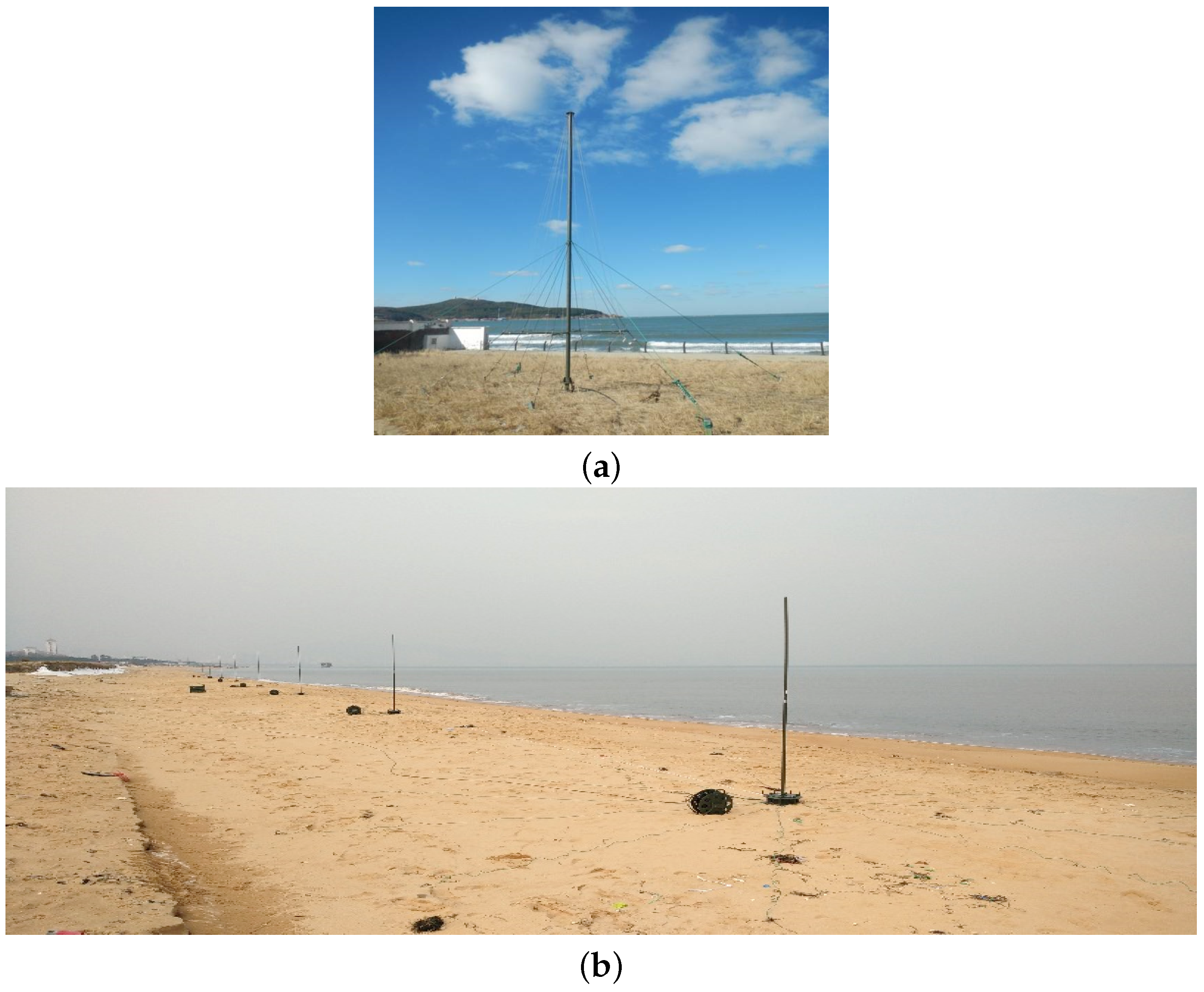
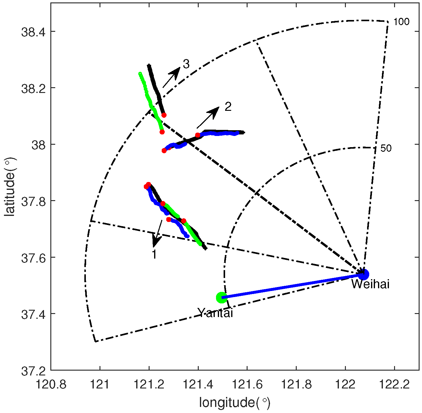
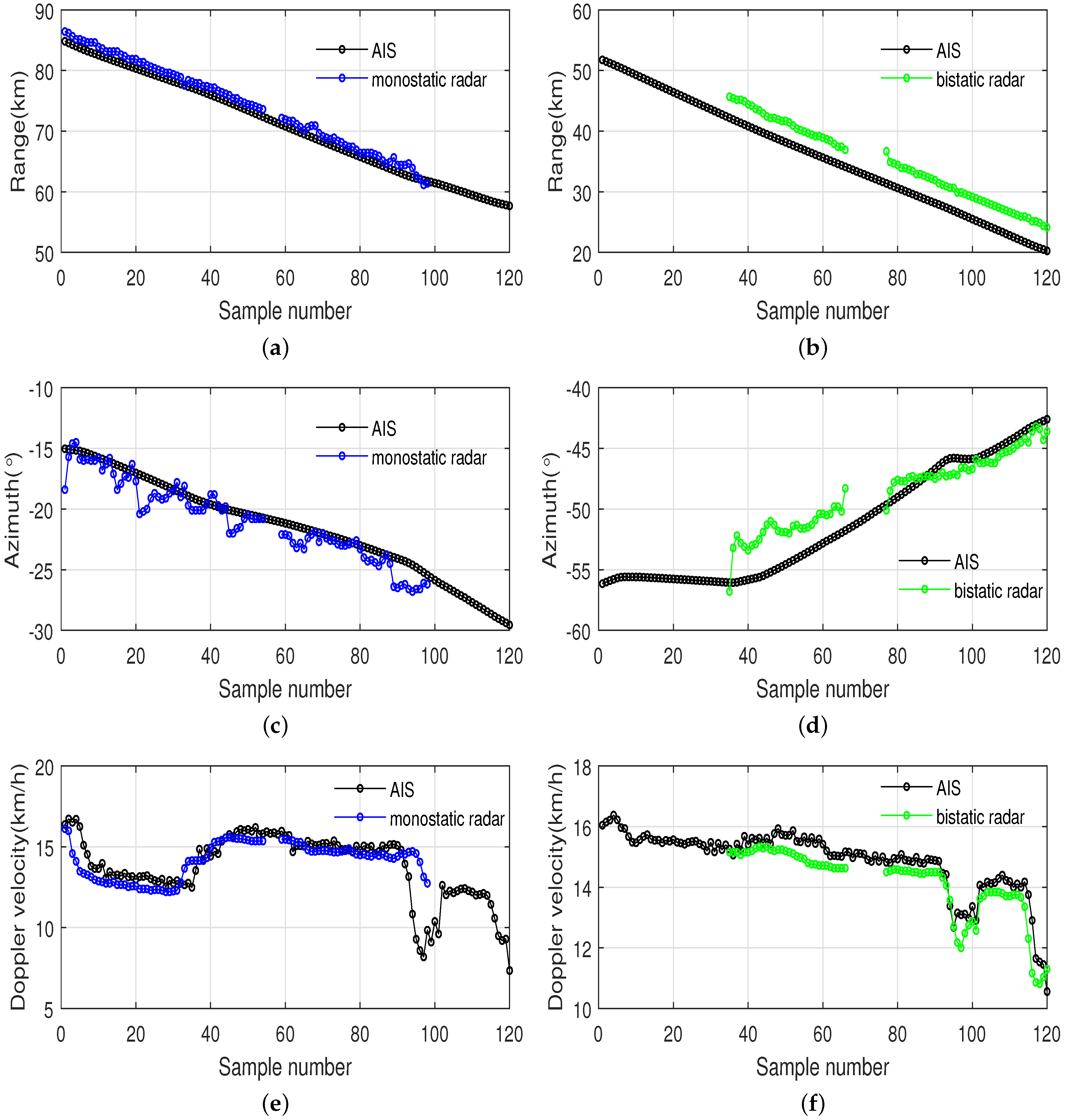
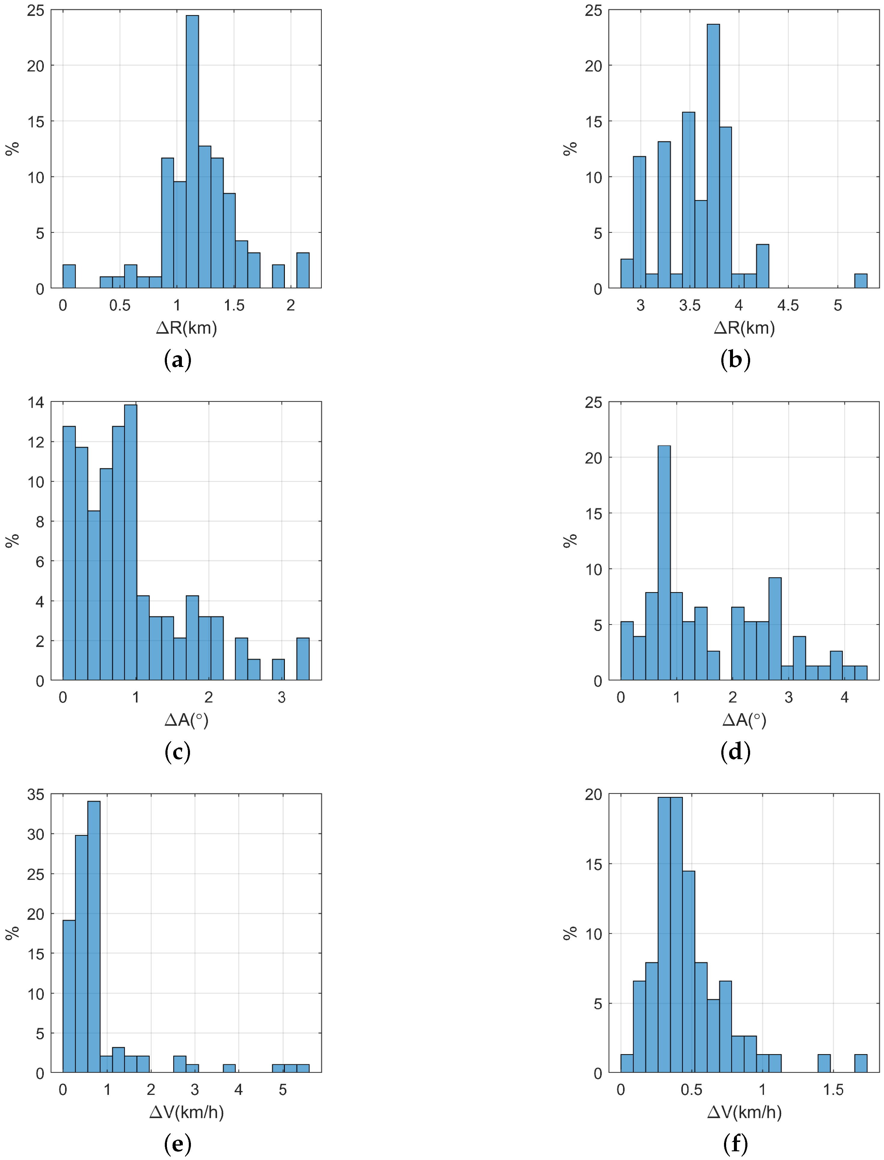
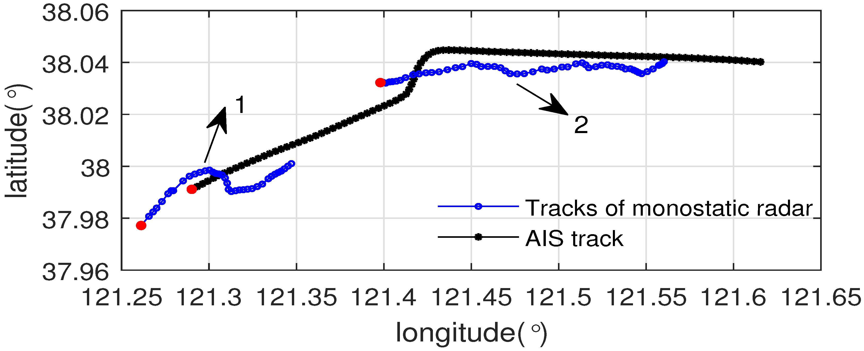
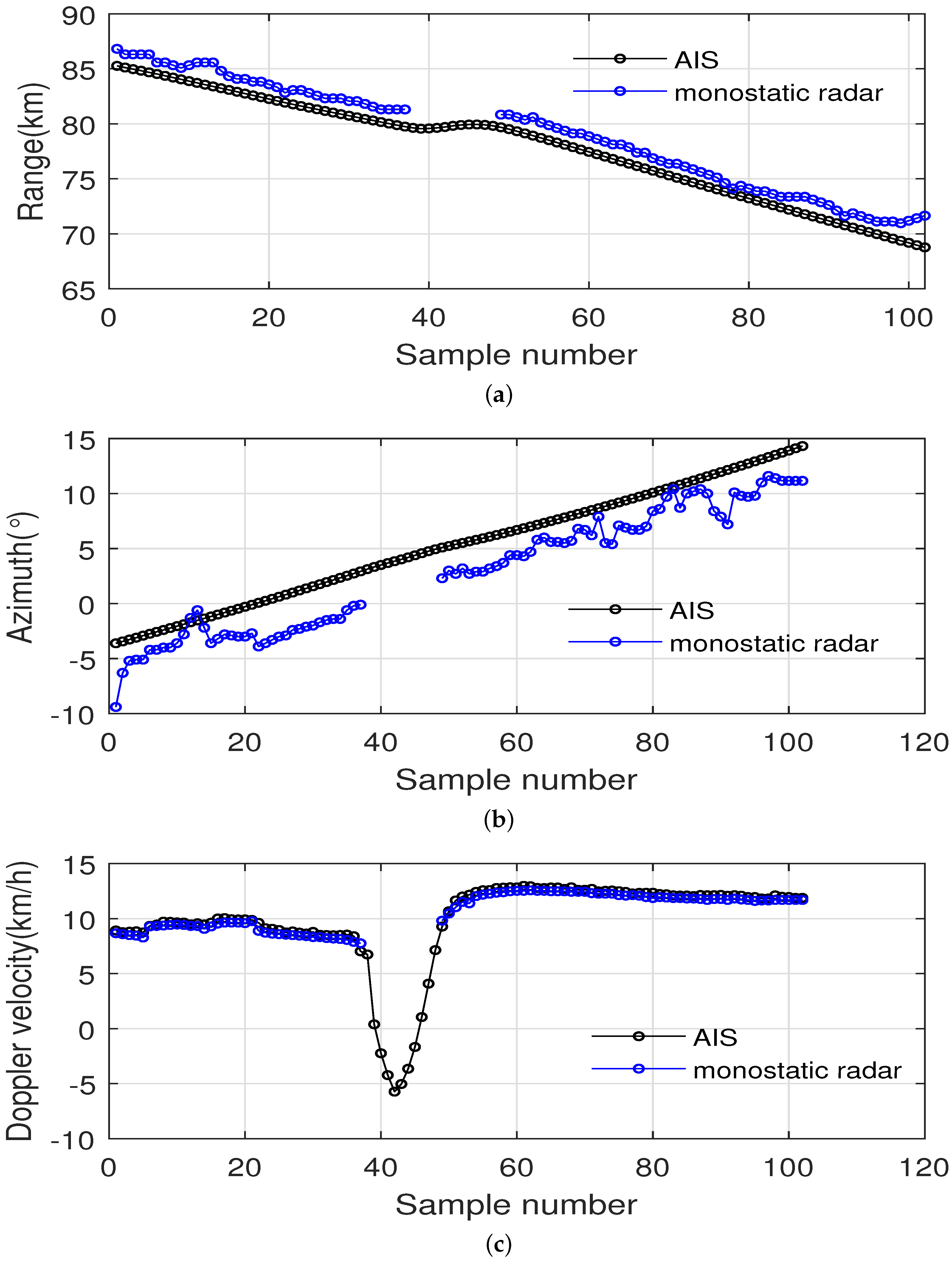
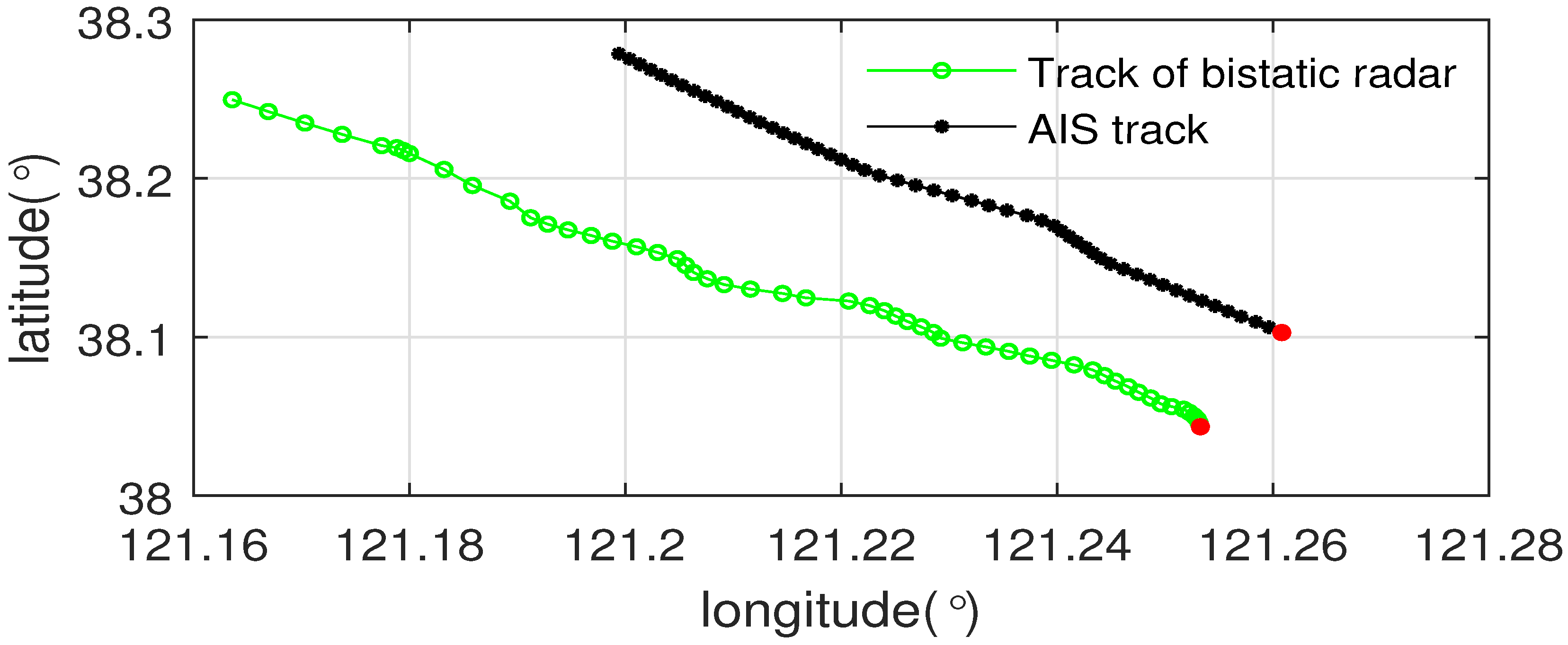
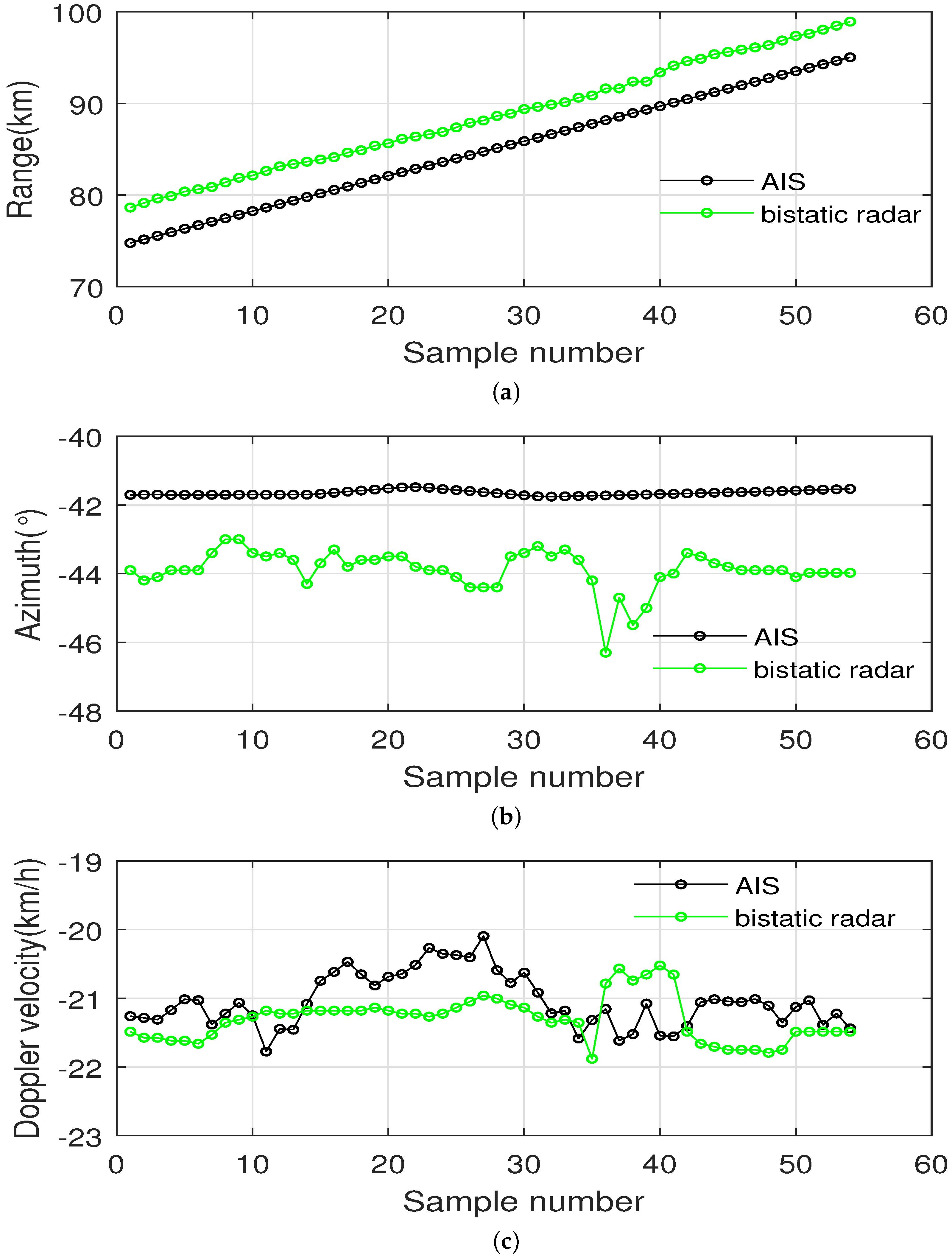
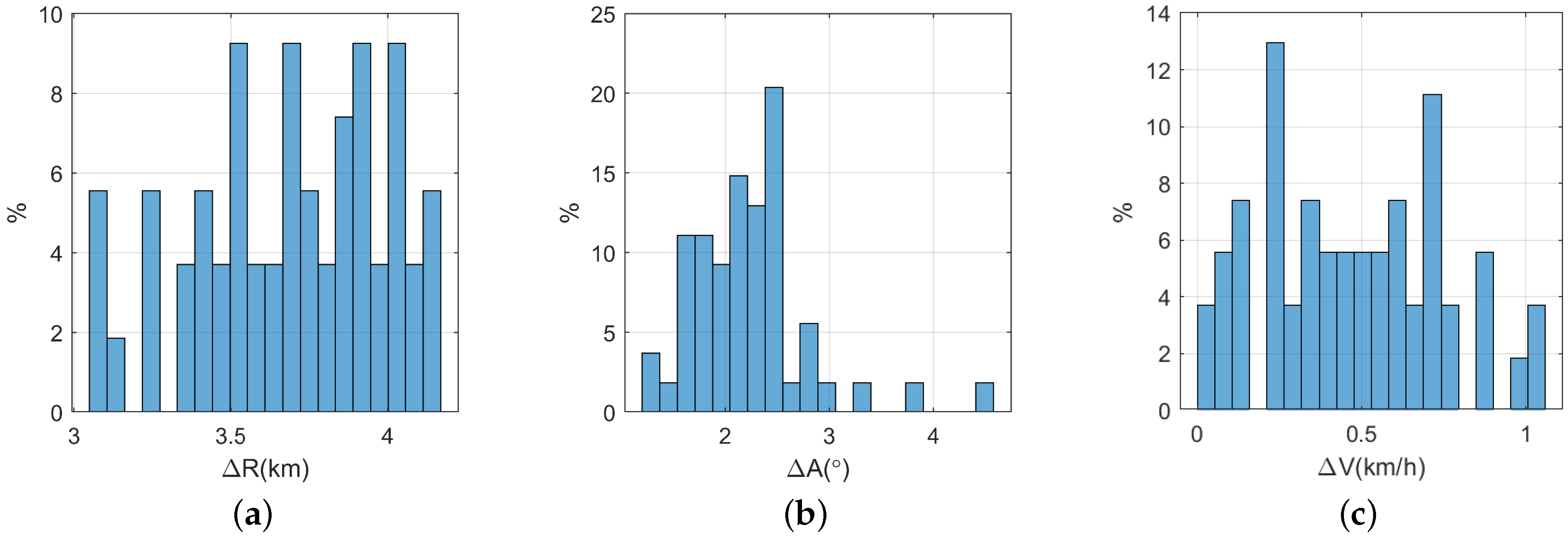
3. Experiment Results

To test the target detection and tracking performance of a bistatic compact HFSWR and verify the effectiveness and applicability of the proposed target tracking method, vessel detection and tracking experiments were conducted using field data simultaneously collected by a newly developed T/R-R compact HFSWR system, as shown in Figure 2, in operation at North China Sea from 9:57 a.m. to 13:42 p.m. on 30 April 2019. The monostatic T/R radar is located at Weihai (122.07 E, 37.54 N), while the other independent receiving station is deployed at Yantai (121.49 E, 37.45 N). The baseline distance L is 52 km, and φ is 10.35 for this configuration.
The compact HFSWR system used a solid-state transmitter with a maximum peak power of 2 kW and linear frequency modulated interrupting continuous wave (FMICW) as its transmitted waveform. A 10-meter-high omnidirectional log-periodic antenna, as shown in Figure 2a, was used to transmit electromagnetic waves with a working frequency of 4.7 MHz. Two similar linear receiving antenna arrays with an antenna element height of 4 meters were placed along the coast at Weihai and Yantai, respectively. Here, only the photo of the receiving antenna array at the Yantai station is shown in Figure 2b. Each receiving antenna array consists of eight active whip antenna units with an inter-element distance of 15 m. Thus, the aperture size of each receiving array is 105 m. The maximum detection range is designed as 100 km. As for vessel detection, the coherent integration time is set to be 262.144 s. A moving slide window method with a window length of 266.144 s is used to produce the detection data. The window slides forward with a step of 60 s, thus the data rate is 1 frame/min. The two radars are synchronized using a GPS time reference. Simultaneous automatic identification system (AIS) data were used as ground truth for comparisons and evaluations [39].
From the data collected by the bistatic compact HFSWR at Yantai, the range sum R and the azimuth θ R of the detected targets were estimated, then their ranges R R were calculated from Equation (2) and the measured state vectors [ R R m θ R m v d R m ] can be obtained. Then the proposed target tracking method was applied to the target detection data to obtain the bistatic target tracks. The target tracking method proposed in [11] was applied to the target plot data sequence measured by the monostatic HFSWR at Weihai to produce the monostatic target tracks. The threshold parameters involved in the tracking algorithm were determined via trial-and-error and they are summarized as follows:
  • Track initiation—M is chosen to be equal to 3, and N is 4.
  • Data association—The validation gate thresholds of range, azimuth, and Doppler velocity for monostatic HFSWR are 1.5 km, 5 , and 1 km/h, while those for bistatic HFSWR are set to 4 km, 5 , and 1.5 km/h, respectively. The weights W w d , W R , and W θ for monostatic radar are 0.6, 0.3, and 0.1, while those for bistatic radar are set to 0.7, 0.2, and 0.1, respectively.
  • Track termination—K is set to be 3 and L is 5. The maximum target velocity v m a x is set to 70 km/h.
From the obtained tracking results, three typical targets are selected for analysis, as shown in Figure 3.
In Figure 3, the blue and green dots indicate the location of the monostatic HFSWR at Weihai and the bistatic HFSWR at Yantai, respectively. The black angular sector illustrates the detection region of the monostatic HFSWR at Weihai. The three targets are marked as ‘1’, ‘2’, and ‘3’ and named as target 1, target 2, and target 3, respectively. The tracks in blue, green, and black represent the tracking results from the monostatic radar, bistatic radar, and matched AIS, respectively. The red dot indicates the first plot of a track. It is shown that target 1 is captured by both the monostatic and bistatic radars simultaneously, target 2 is tracked by the monostatic radar only, and target 3 is only detected by the bistatic radar. The general information of these three targets reported by AIS are listed in Table 1, and their photos are shown in Figure 4.
The tracking results of these three targets are analyzed and compared in detail as follows.
(1) Target tracks obtained by both the monostatic and bistatic radars.
As shown in Figure 3, target 1 moves nearly along the bistatic bisector direction of the bistatic radar at Yantai, its velocities have significant projection components in the radial direction of the monostatic radar at Weihai. Thus, it is captured by both radars. The tracks in longitudes and latitudes of target 1 are shown in Figure 5.
It can be seen from Figure 5 that the obtained tracks from both the bistatic radar and monostatic radar are broken into two track segments. The four track segments are marked as ‘1’, ‘2’, ’3’, and ‘4’, whose durations were 10:38–11:32 a.m. for track segment 1 with 54 plots, 11:13–11:44 a.m. for track segment 2 with 32 plots, 11:37 a.m.–12:16 p.m. for track segment 3 with 40 plots, and 11:54 a.m.–12:37 p.m. for track segment 4 with 44 plots. The duration for the matched AIS track was from 10:38 a.m. to 12:37 p.m. with 120 plots. It is shown that these four track segments together cover the entire AIS track.
In order to quantitatively evaluate the tracking performance, the positions provided by the AIS track in longitudes and latitudes, as well as the velocities, were projected onto the coordinates of the monostatic radar at Weihai and bistatic radar at Yantai, respectively, to obtain the corresponding range data, azimuth data, and Doppler velocity data sequences. The root-mean-square error (RMSE) and statistical error distribution criteria were used for accuracy evaluation.
The range data, azimuth data, and Doppler velocity data sequences corresponding to the four track segments are compared with those obtained by the AIS track projections, the results are shown in Figure 6. Figure 6a,c,e illustrate the range, azimuth, and Doppler velocity comparison results of the monostatic radar, respectively. The corresponding comparison results of the bistatic radar are shown in Figure 6b,d,f, respectively. The Sample number denotes the sequence number of a plot in a track.
As the monostatic radar at Weihai and bistatic radar at Yantai measure targets under different coordinates, the scales of their kinematic parameters are different. According to the velocities reported by AIS, target 1 moves at a nearly constant velocity during the observation period. However, the instability of the instantaneously measured course results in fluctuations in radial velocity projections. It can be observed that the range data, azimuth data, and Doppler velocity data sequences obtained from track segment 1 and track segment 3 of the monostatic compact HFSWR are in good agreement with those of the AIS results, the corresponding RMSEs are 1.24 km, 1.18 , and 1.3 km/h, respectively. By contrast, the range and azimuth data sequences obtained from track segment 2 and track segment 4 of the bistatic compact HFSWR agree well with those of the AIS results, with a relatively larger RMSEs of 3.6 km and 1.94 , respectively. It is worth noting that the agreement between the bistatic Doppler velocity data sequences and the projected results of AIS is fairly good, with a RMSE of 0.55 km/h. For clarity, the results are listed in Table 2.
The error distributions of the range, azimuth, and Doppler velocity data sequences of target 1 for both monostatic and bistatic HFSWR are illustrated in Figure 7 for more detailed analysis.
It can be seen from Figure 7 that the majority of range error, azimuth error, and Doppler velocity error for monostatic HFSWR are less than 1.5 km, 2 , and 1 km/h, respectively, while those for bistatic HFSWR are less than 4 km, 3 , and 1 km/h, respectively.
The above results indicate that the monostatic radar achieves better tracking accuracy than that of the bistatic radar for target 1. However, the RMSE of the Doppler velocity from bistatic HFSWR is lower than that of monostatic HFSWR. The azimuth estimation results from both monostatic radar and bistatic radar display some random fluctuations due to the coarse azimuth resolution caused by reduced aperture size. It is worth mentioning that the range accuracy is different for monostatic radar and bistatic radar. The range resolution of the CORMS is designed to be 2.5 km. The range accuracy of the monostatic radar is much higher than this value as reported in [11], while the range accuracy of the bistatic radar is worse than this design value because the calculated ranges are affected by error in azimuth estimations.
It can also be observed that the three kinematic parameters between track segment 1 and track segment 3, as well as between track segment 2 and track segment 4 are consistent. The track fragmentation is probably due to the missed detections at some sampling time, which may be caused by the weak returned echos due to the relatively smaller ship size, or sea clutter interference, etc. Combining the simultaneous target detections of a monostatic and bistatic radar, the overlapped discontinuous track segments belonging to the same target can be bridged together to obtain a longer track. Thus, there is a potential for this radar configuration to maintain better track consistence.
(2) Target tracks obtained only by the monostatic radar.
As a Doppler radar, HFSWR favors detecting targets that have significant velocity projection components along its radial directions. The track of target 2 can only be produced from the monostatic radar data as it sails nearly along the tangent direction of the isorange ellipse of the bistatic radar. The obtained two track segments, marked as ‘1’ and ‘2’, and the matched AIS track are illustrated in Figure 8. The durations of these two track segments are 11:52 a.m.–12:28 p.m. for track segment 1 with 37 plots, 12:40–1:33 p.m. for track segment 2 with 54 plots. The duration for the matched AIS track is from 11:52 a.m. to 1:33 p.m. with 102 plots.
The comparisons of the corresponding range data, azimuth data, and Doppler velocity data sequences are shown in Figure 9. It is observed that both the range data and Doppler velocity data sequences agree well with those of the AIS projection results with RMSEs of 1.37 km, and 0.36 km/h, respectively, which are similar to the results obtained by the monostatic radar for target 1. However, the accuracy of the azimuth data sequence is a little worse with an RMSE of 2.66 due to the target’s longer distance from the radar site, which leads to large target position deviations from its true trajectory. It can be seen from Figure 9c that the Doppler velocity changes from positive values to negative ones, and then becomes positive again around the 40th plots. This is because that target 2 moves nearly along the tangent direction of the Weihai radar. At some locations, its Doppler velocity becomes nearly zero and thus it is difficult to be detected. The missed detections may lead to the track fragmentation. However, the tracking algorithm adopted here has not been considered such situations.
The error distributions of the range, azimuth, and Doppler velocity data sequences of target 2 for monostatic HFSWR are illustrated in Figure 10 for more detailed analysis.
It can be seen from Figure 10 that the majority of range error, azimuth error, and Doppler velocity error for monostatic HFSWR are less than 1.5 km, 4 , and 0.6 km/h, respectively.
(3) Target track obtained only by the bistatic radar.
It can be seen from Figure 3 that target 3 goes beyond the maximum detection range of 100 km of the monostatic radar at Weihai. Fortunately, it is still within the detection range of the bistatic radar at Yantai. Thus, it is only captured by the bistatic radar. From this perspective, the coverage area of the monostatic radar is expanded. The obtained track, as well as its matched AIS track, whose duration are from 10:11 a.m. to 11:08 a.m. with 58 plots, are shown in Figure 11. It is observed that the track obtained by the bistatic radar deviates from its true trajectory but shows a similar course with that of AIS.
The kinematic comparisons of the corresponding range data, azimuth data, and Doppler velocity data sequences are shown in Figure 12.
Compared with the results provided by AIS, it can be noted that the range errors are nearly constant for all the plots with an RMSE of 3.7 km and a standard deviation of 0.3 km. The azimuth data of AIS keep nearly constant, while the azimuth data sequence of the bistatic radar presents fluctuations with an RMSE of 2.3 and a maximum deviation of 4.58 . The RMSE of Doppler velocity is 0.55 km/h and the maximum deviation is 1.05 km/h, indicating again that a bistatic HFSWR can measure the Doppler velocity of a target with high accuracy.
The error distributions of the range, azimuth, and Doppler velocity data sequences of target 3 for bistatic HFSWR are illustrated in Figure 13 for more detailed analysis.
It can be seen from Figure 13 that the majority of range error, azimuth error, and Doppler velocity error for monostatic HFSWR are less than 4 km, 3 , and 1 km/h, respectively.

4. Discussion

By analyzing the tracking results from the developed monostatic and bistatic compact HFSWR for three targets considered here, it can be summarized that:
(i) Both monostatic and bistatic compact HFSWR can produce target tracks, simultaneously or complementarily. However, the tracks obtained by compact HFSWR are usually fragmented into short track segments due to the lower detection rate, clutter interference, etc. With the T/R-R configuration, there are potentials that the simultaneously obtained tracks can be fused to improve the tracking accuracy, and the complementary tracks can be associated to enhance the track consistence. Specific track association and fusion methods should be developed to achieve this goal.
(ii) The azimuth and Doppler velocity estimation accuracies of monostatic and bistatic HFSWR are comparable. However, the range estimation accuracy and the resulting tracking accuracy of bistatic HFSWR is relatively lower than those of the monostatic HFSWR. The effect of θ R on the estimation accuracy of R R is significant. It is worth developing a method to mitigate the measurement error due to the reduced azimuth resolution of a compact radar. The coupling characteristic between range and azimuth should be fully considered in designing superior tracking algorithms.
(iii) The coverage area of a monostatic HFSWR can be extended by a T/R-R configuration with only a little extra cost.

5. Conclusions

The target detection and tracking performance of a bistatic compact HFSWR was investigated in this paper. An applicable target tracking method for bistatic compact HFSWR was proposed and its performance was verified using the field data collected simultaneously by a monostatic and a bistatic HFSWRs sharing the same transmitter. The experiment results demonstrate that the bistatic HFSWR can produce target tracks with acceptable errors. Moreover, the tracking results of the bistatic HFSWR were compared with those of a monostatic HFSWR. It is found that the range estimation accuracy, thus the tracking accuracy of a bistatic HFSWR is lower than that of a monostatic one based on the data in this work. The combination of a monostatic HFSWR and a bistatic HFSWR provides target observations from different perspectives, thus, the T/R-R configuration can obtain synchronous as well as complementary information for the same target. This configuration may be potentially exploited to increase the target detection probability, improve the target detection and tracking accuracy, and enhance the track continuity. Also, the T/R-R configuration can increase the detection range and extend the coverage area, thus more targets can be monitored.
In the future, more data should be collected by the T/R-R compact HFSWR so that enough statistical sample can be used to determine how long a track should be maintained based on predictions only. According to our experience, improper selection of the termination criteria will lead to track fragmentation. In our experiments, it is found that the fragmentation phenomenon appears more often for the bistatic radar than the monostatic radar. The effect of the parameters involved in the bistatic tracking algorithm on the tracking performance also needs to be studied. Moreover, new track association and fusion methods will be developed to associate and merge the track segments simultaneously obtained by the monostatic radar and bistatic radar into a longer track to improve the continuity as well as the accuracy of target tracking with compact HFSWR.

Author Contributions

Conceptualization, W.S. and W.H.; methodology, W.S. and M.J.; software, W.S.; validation, W.S., W.H., and Y.J.; formal analysis, W.S. and W.H.; investigation, M.J.; resources, Y.J. and Y.D.; data curation, Y.J.; writing—original draft preparation, W.S.; writing—review and editing, W.H.; visualization, M.J.; supervision, W.H. and Y.D.; project administration, W.S.; funding acquisition, W.S. All authors have read and agreed to the published version of the manuscript.

Funding

This research was funded by the National Key R&D Program of China with grant number 2017YFC1405202, National Natural Science Foundation of China with grant numbers 61501520, 61831010, 61671166, the Fundamental Research Funds for the Central Universities with grant numbers 19CX02046A, 17CX02079, and CSC scholarship for 1-year research abroad at Memorial University.

Acknowledgments

The authors would like to thank the anonymous reviewers for their comments and suggestions that helped to improve the quality of this article.

Conflicts of Interest

The authors declare no conflict of interest.

Abbreviations

The following abbreviations are used in this manuscript:
HFSWRHigh-Frequency Surface Wave Radar
MUSICMultiple SIgnal Classfication
MIMOMultiple-Input Multiple-Output
MTTMulti-Target Tracking
DBFDigital Beam Forming
CMKFConverted Measurement Kalman Filter
AISAutomatic Identification System
RMSERoot Mean Square Error

References

  1. Sevgi, L.; Ponsford, A.; Chan, H.C. An integrated maritime surveillance system based on high-frequency surface-wave radars. 1. Theoretical background and numerical simulations. IEEE Antenn. Propag. Mag. 2001, 43, 28–43. [Google Scholar] [CrossRef]
  2. Green, D.; Gill, E.; Huang, W. An inversion method for extraction of wind speed from high-frequency ground-wave radar. IEEE Trans. Geosci. Remote Sens. 2009, 47, 3530–3549. [Google Scholar] [CrossRef]
  3. Ponsford, A.M.; Wang, J. A review of high frequency surface wave radar for detection and tracking of ships. Turk. J. Elect. Eng. Comput. Sci. 2010, 18, 409–428. [Google Scholar]
  4. Park, S.; Cho, C.J.; Ku, B.; Lee, S.; Ko, H. Compact HF surface wave radar data generating simulator for ship detection and tracking. IEEE Geosci. Remote Sens. Lett. 2017, 14, 969–973. [Google Scholar] [CrossRef]
  5. Roarty, H.J.; Lemus, E.R.; Handel, E.; Glenn, S.M.; Barrick, D.E.; Isaacson, J. Performance evaluation of SeaSonde high-frequency radar for vessel detection. Mar. Technol. Soc. J. 2011, 45, 14–24. [Google Scholar] [CrossRef]
  6. Smith, M.; Roarty, H.J.; Glenn, S.; Whelan, C.; Barrick, D.E.; Isaacson, J. Methods of associating CODAR SeaSonde vessel detection data into unique tracks. In Proceedings of the MTS/IEEE Oceans, San Diego, CA, USA, 23–27 September 2013; pp. 1–5. [Google Scholar]
  7. Lu, B.; Wen, B.; Tian, Y.; Wang, R. A vessel detection method using compact-array HF radar. IEEE Geosci. Remote Sens. Lett. 2017, 14, 2017–2021. [Google Scholar] [CrossRef]
  8. Helzel, T.; Hansen, B.; Kniephphoff, M.; Petersen, L.; Valentin, M. Introduction of the compact HF radar WERA-S. In Proceedings of the IEEE/OES Baltic International Symposium, Klaipeda, Lithuania, 8–10 May 2012; pp. 1–3. [Google Scholar]
  9. Ji, Y.; Zhang, J.; Wang, Y.; Sun, W.; Li, M. Target monitoring using small-aperture compact high-frequency surface wave radar. IEEE Aerosp. Electron. Syst. Mag. 2018, 33, 22–31. [Google Scholar] [CrossRef]
  10. Sun, W.; Huang, W.; Ji, Y.; Dai, Y.; Ren, P.; Zhou, P. Vessel tracking with small-aperture compact high-frequency surface wave radar. In Proceedings of the MTS/IEEE Oceans, Marseille, France, 17–20 June 2019; pp. 1–4. [Google Scholar]
  11. Sun, W.; Huang, W.; Ji, Y.; Dai, Y.; Ren, P.; Zhou, P.; Hao, X. A vessel azimuth and course joint re-estimation method for compact HFSWR. IEEE Trans. Geosci. Remote Sens. 2020, 58, 1041–1051. [Google Scholar] [CrossRef]
  12. Yao, G.; Xie, J.; Huang, W. First-order ocean surface cross section for shipborne HFSWR incorporating a horizontal oscillation motion model. IET Radar Sonar Navig. 2018, 12, 973–978. [Google Scholar] [CrossRef]
  13. Chen, Z.; He, C.; Zhao, C.; Xie, F. Enhanced target detection for HFSWR by 2-D MUSIC based on sparse recovery. IEEE Geosci. Remote Sens. Lett. 2017, 14, 1983–1987. [Google Scholar] [CrossRef]
  14. Barca, P.; Maresca, S.; Grasso, R.; Bryan, K.; Horstmann, J. Maritime surveillance with multiple over-the-horizon HFSW radars: An overview of recent experimentation. IEEE Aerosp. Electron. Syst. Mag. 2015, 30, 4–18. [Google Scholar] [CrossRef]
  15. Lesturgie, M. Improvement of high-frequency surface waves radar performances by use of multiple-input multiple-output configurations. IET Radar Sonar Navig. 2008, 3, 49–61. [Google Scholar] [CrossRef]
  16. Anderson, S.J.; Edwards, P.J.; Marrone, P.; Abramovich, Y.I. Investigations with SECAR- a bistatic HF surface wave radar. In Proceedings of the 2003 International Conference on Radar, Adelaide, Australia, 3–5 September 2003; pp. 717–722. [Google Scholar]
  17. Marrone, P.; Edwards, P. The case for bistatic HF surface wave radar. In Proceedings of the 2008 Proceedings of the International Conference on Radar, Adelaide, Australia, 2–5 September 2008; pp. 633–638. [Google Scholar]
  18. Anderson, S.J. Optimizing HF Radar Siting for Surveillance and Remote Sensing in the Strait of Malacca. IEEE Geosci. Remote Sens. Lett. 2012, 51, 1805–1816. [Google Scholar] [CrossRef]
  19. Xie, J.; Sun, M.; Ji, Z. Space-time model of the first-order sea clutter in onshore bistatic high frequency surface wave radar. IET Radar Sonar Navig. 2015, 9, 55–61. [Google Scholar] [CrossRef]
  20. Wang, J.; Dizaji, R.; Ponsford, A.M. Analysis of clutter distribution in bistatic high frequency surface wave radar. In Proceedings of the Canadian Conference on Electrical and Computer Engineering, Ontario, QC, Canada, 2–5 May 2004; pp. 1301–1304. [Google Scholar]
  21. Liu, C.; Chen, B.; Zhang, S. Co-channel interference suppression by time and range adaptive processing in bistatic high-frequency surface wave synthesis impulse and aperture radar. IET Radar Sonar Navig. 2009, 3, 638–645. [Google Scholar] [CrossRef]
  22. Gill, E.; Walsh, J. High frequency bistatic cross section of the ocean surface. Radio Sci. 2001, 36, 1459–1476. [Google Scholar] [CrossRef]
  23. Gill, E.; Huang, W.; Walsh, J. The effect of the bistatic scattering angle on the high-frequency radar cross sections of the ocean surface. IEEE Geosci. Remote Sens. Lett. 2008, 5, 143–146. [Google Scholar] [CrossRef]
  24. Ma, Y.; Gill, E.; Huang, W. Bistatic high-frequency radar ocean surface cross section incorporating a dual-frequency platform motion model. IEEE J. Ocean. Eng. 2018, 43, 205–210. [Google Scholar] [CrossRef]
  25. Ma, Y.; Huang, W.; Gill, E. Bistatic high frequency radar ocean surface cross section for an FMCW source with an antenna on a floating platform. Int. J. Antennas Propag. 2016, 2016, 8675964. [Google Scholar] [CrossRef] [Green Version]
  26. Ma, Y.; Gill, E.; Huang, W. First-Order Bistatic high-Frequency radar ocean surface cross-section for an antenna on a floating platform. IET Radar Sonar Navig. 2016, 10, 1136–1144. [Google Scholar] [CrossRef] [Green Version]
  27. Gill, E.; Huang, W.; Walsh, J. On the development of a second-order bistatic radar cross section of the ocean surface—A high-frequency result for a finite scattering patch. IEEE J. Ocean. Eng. 2006, 31, 740–750. [Google Scholar] [CrossRef]
  28. Ma, Y.; Huang, W.; Gill, E. The second-order bistatic high frequency radar ocean surface cross section for an antenna on a floating platform. Can. J. Remote Sens. 2016, 42, 332–343. [Google Scholar] [CrossRef]
  29. Lipa, B.; Whelan, C.; Rector, B.; Nyden, B. HF radar bistatic measurement of surface current velocities: Drifter comparisons and radar consistency checks. Remote Sens. 2009, 1, 1190–1211. [Google Scholar] [CrossRef] [Green Version]
  30. Yang, J.; Wen, B.; Zhang, C.; Huang, X.; Yan, Z.; Shen, W. A bistatic HF radar for surface current mapping. IEICE Electron. Expr. 2010, 7, 1435–1440. [Google Scholar] [CrossRef] [Green Version]
  31. Trizna, D.B. A bistatic HF radar for current mapping and robust ship tracking. In Proceedings of the MTS/IEEE Oceans, Quebec City, QC, Canada, 15–18 September 2008; pp. 1–6. [Google Scholar]
  32. Hardman, R.L.; Wyatt, L.R.; Engleback, C.C. Measuring the directional ocean spectrum from simulated bistatic HF radar data. Remote Sens. 2020, 12, 313. [Google Scholar] [CrossRef] [Green Version]
  33. Huang, W.; Gill, E.; Wu, X.; Li, L. Measurement of sea surface wind direction using bistatic high-frequency radar. IEEE Trans. Geosci. Remote Sens. 2012, 50, 4117–4122. [Google Scholar] [CrossRef]
  34. Chan, H.C.; Davies, T.W.; Hall, P. Iceberg tracking using HF surface wave radar. In Proceedings of the MTS/IEEE Oceans, Halifax, NS, Canada, 6–9 October 1997; pp. 1290–1296. [Google Scholar]
  35. Vivone, G.; Braca, P.; Horstmann, P. Knowledge-based multi-target ship tracking for HF surface wave radar systems. IEEE Trans. Geosci. Remote Sens. 2015, 53, 3931–3949. [Google Scholar] [CrossRef] [Green Version]
  36. Braca, P.; Marano, S.; Matta, V.; Willett, P. Asymptotic efficiency of the PHD in multitarget/multisensor estimation. IEEE J. Sel. Top. Signal Process. 2013, 7, 553–564. [Google Scholar] [CrossRef]
  37. Zong, H.; Yu, C.; Zhou, G.; Quan, T. Track initiation in monostatic-bistatic composite high frequency surface wave radar network based on NFE model. In Proceedings of the 2010 International Conference on Electronics and Information Engineering, Kyoto, Japan, 1–3 August 2010; pp. 81–85. [Google Scholar]
  38. Bar-Shalom, Y.; Willett, P.; Tian, X. Tracking and Data Fusion: A Handbook of Algorithms; YBS Publishing: Storrs, CT, USA, 2011. [Google Scholar]
  39. Nikolic, D.; Stojkovic, N.; Lekic, N. Maritime over the horizon sensor integration: High frequency surface-wave-radar and automatic identification system data integration algorithm. Sensors 2018, 18, 1147. [Google Scholar] [CrossRef] [Green Version]
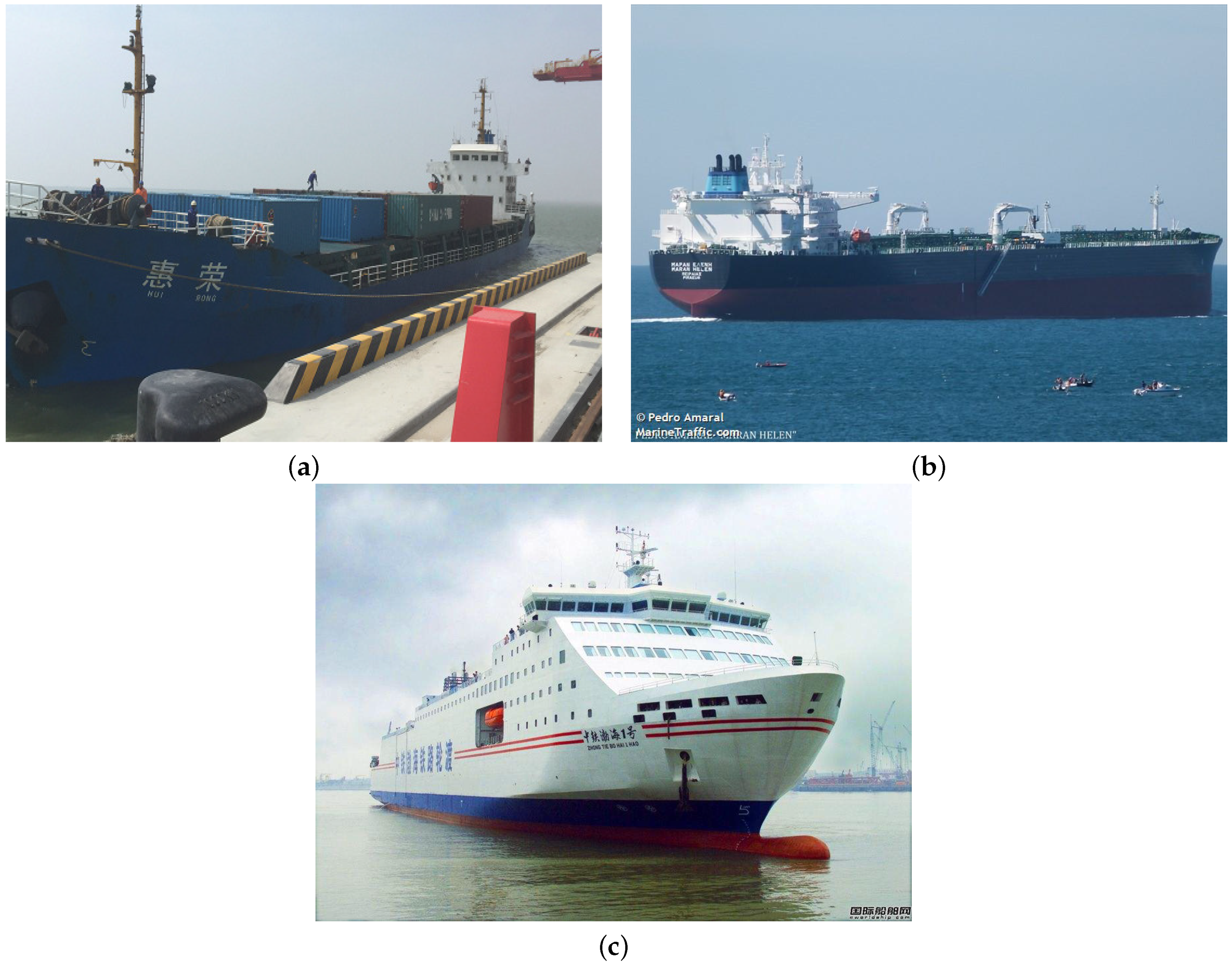
Figure 1. The radar configuration geometry of a T/R-R high-frequency surface wave radar (HFSWR) system. The transmitter and receiving array 1 are deployed at the transmitting station (Tx), while receiving array 2 is deployed at the receiving station (Rx). The transmitter serves the two receiving arrays simultaneously. The distance L between the transmitter and receiver is called the bistatic range or simply the baseline. φ denotes the angle between the baseline and East direction. Denote ψ T and ψ R , respectively, as the radar look directions of receiving array 1 and receiving array 2 with respect to true North. β is the bistatic angle.
Remotesensing 12 01266 g001
Figure 2. Transmitting antenna and one receiving antenna array of the developed T/R-R compact HFSWR system. (a) Transmitting antenna installed at Weihai radar station. (b) One receiving antenna array.
Remotesensing 12 01266 g002
Figure 3. Tracking results of three typical targets. The blue and green dots indicate the location of the monostatic HFSWR at Weihai and the bistatic HFSWR at Yantai, respectively. The black angular sector illustrates the detection region of the monostatic HFSWR at Weihai. The three targets are marked as ‘1’, ‘2’, and ‘3’ and named as target 1, target 2, and target 3, respectively. The tracks in blue, green, and black represent the tracking results from the monostatic radar, bistatic radar, and matched AIS, respectively. The red dot indicates the first plot of a track.
Remotesensing 12 01266 g003
Figure 4. Photos of three targets considered in this paper. (a) Target 1—HUI RONG, the photo is from the website: www.yantaiport.com.cn. (b) Target 2—MARAN HELEN, the photo is from: www.marinetraffic.com. (c) Target 3—ZHONGTIEBOHAI 1 HAO, the photo is from: image.baidu.com.
Remotesensing 12 01266 g004
Figure 5. Comparison between radar tracks and automatic identification system (AIS) track of target 1.
Remotesensing 12 01266 g005
Figure 6. Kinematic parameter comparisons for target 1. (a) Range comparison for monostatic radar. (b) Range comparison for bistatic radar. (c) Azimuth comparison for monostatic radar. (d) Azimuth comparison for bistatic radar. (e) Doppler velocity comparison for monostatic radar. (f) Doppler velocity comparison for bistatic radar.
Remotesensing 12 01266 g006
Figure 7. Kinematic parameter error distributions for target 1. (a) Range error distribution for monostatic radar. (b) Range error distribution for bistatic radar. (c) Azimuth error distribution for monostatic radar. (d) Azimuth error distribution for bistatic radar. (e) Doppler velocity error distribution for monostatic radar. (f) Doppler velocity error distribution for bistatic radar.
Remotesensing 12 01266 g007
Figure 8. Track comparison between monostatic radar and AIS of target 2.
Remotesensing 12 01266 g008
Figure 9. Kinematic parameter comparisons for target 2. (a) Range comparison for monostatic radar. (b) Azimuth comparison for monostatic radar. (c) Doppler velocity comparison for monostatic radar.
Remotesensing 12 01266 g009
Figure 10. Kinematic parameter error distributions for target 2. (a) Range error distribution. (b) Azimuth error distribution. (c) Doppler velocity error distribution.
Remotesensing 12 01266 g010
Figure 11. Track comparison between bistatic radar and AIS of target 3.
Remotesensing 12 01266 g011
Figure 12. Kinematic parameter comparisons for target 3. (a) Range comparison for bistatic radar. (b) Azimuth comparison for bistatic radar. (c) Doppler velocity comparison for bistatic radar.
Remotesensing 12 01266 g012
Figure 13. Kinematic parameter error distributions for target 3. (a) Range error distribution. (b) Azimuth error distribution. (c) Doppler velocity error distribution.
Remotesensing 12 01266 g013
Table 1. General information for three targets.
Target 1Target 2Target 3
MMSI413331140241491000412328490
Ship NameHUI RONGMARAN HELENZHONGTIEBOHAI 1 HAO
Ship TypeCargoTankerPassenger
Length (m)98274182
Width (m)164625
Draught (m)3.99.46.0
Table 2. Root-mean-square error (RMSE) of range, azimuth and Doppler velocity for target 1.
Range (km)Azimuth ( )Doppler velocity (km/h)
Monostatic radar1.241.181.30
Bistatic radar3.601.940.55

