Article

Machine Learning Based On-Line Prediction of Soil Organic Carbon after Removal of Soil Moisture Effect

by
Said Nawar
1,2,
Muhammad Abdul Munnaf
1 and
Abdul Mounem Mouazen
1,*
1
Department of Environment, Faculty of Bioscience Engineering, Ghent University, Coupure Links 653, 9000 Ghent, Belgium
2
Soil and Water Department, Faculty of Agriculture, Suez Canal University, Ismailia 41522, Egypt
*
Author to whom correspondence should be addressed.
Remote Sens. 2020, 12(8), 1308; https://doi.org/10.3390/rs12081308
Submission received: 30 March 2020 / Revised: 16 April 2020 / Accepted: 17 April 2020 / Published: 21 April 2020

Abstract

:
It is well-documented in the visible and near-infrared reflectance spectroscopy (VNIRS) studies that soil moisture content (SMC) negatively affects the prediction accuracy of soil attributes. This work was undertaken to remove the negative effect of SMC on the on-line prediction of soil organic carbon (SOC). A mobile VNIR spectrophotometer with a spectral range of 305–1700 nm and spectral resolution of 1 nm (CompactSpec, Tec5 Technology, Germany) was used for the spectral measurements at four farms in Flanders, Belgium. A total of 381 fresh soil samples were collected and divided into a calibration set (264) and a validation set (117). The validation samples were processed (air-dried and grind) and scanned with the same spectrophotometer in the laboratory. Three SMC correction methods, namely, external parameter orthogonalization (EPO), piecewise direct standardization (PDS), and orthogonal signal correction (OSC) were used to correct the on-line fresh spectra based-on its corresponding laboratory spectra. Then, the Cubist machine learning method was used to develop calibration models of SOC using the on-line spectra (after correction) of the calibration set. Results indicated that the EPO-Cubist outperformed the PDS-Cubist and the OSC-Cubist, with considerable improvements in the prediction results of SOC (coefficient of determination (R2) = 0.76, ratio of performance to deviation (RPD) = 2.08, and root mean square error of prediction (RMSEP) = 0.12%), compared with the corresponding uncorrected on-line spectra (R2 = 0.55, RPD = 1.24, and RMSEP = 0.20%). It can be concluded that SOC can be accurately predicted on-line using the Cubist machine learning method, after removing the negative effect of SMC with the EPO method.

Graphical Abstract

1. Introduction

Organic matter and consequentially soil organic carbon (SOC) are key components of soil that affect its physicochemical properties such as soil structure, water holding capacity, and cation exchange capacity (CEC) [1], in addition to its direct influence on soil resistance to erosion [2]. Therefore, the spatial measurement of SOC content is essential for a wide range of environmental and agricultural applications [3]. Traditional laboratory procedures for determining SOC is costly, destructive, and time-consuming. Therefore, there is an increasing need for rapid, cost-effective, nondestructive, and sufficiently accurate approaches for predicting SOC under field conditions using either portable or on-line sensing infrastructure [4,5].
Visible and near infrared reflectance spectroscopy (VNIRS) is reported to be a promising technology for soil analysis [4,6]. Due to the availability of robust and portable detectors, VNIRS has been widely used for the in situ off-line and on-line predictions of various soil properties [7,8,9] including SOC [10,11]. SOC is indeed a key parameter widely used for soil quality assessment and is considered as one of the most commonly and successfully predicted parameters using VNIRS due not only to the direct spectral response SOC has in the NIR spectral range, but changes in the soil color that are associated with changes in the soil organic matter content detectable in the visible (VIS) range [4,12,13]. Once the spectral features have been calibrated for SOC prediction using chemometrics or machine learning techniques, VNIRS can provide a rapid and cost-effective estimation of SOC in field conditions.
It is important to note that under field conditions, external parameters such as soil moisture content (SMC), temperature, and texture greatly but negatively affect the VNIRS prediction accuracy. The negative influence of SMC on the VNIRS has been reported by several researchers [14,15,16]. Variability in SMC during field measurement can be of significant effect, while under laboratory scanning conditions, the effect of SMC can be diminished by means of scanning soil samples after standard laboratory pretreatments including air drying, grinding, and sieving. Several studies reported a successful VNIRS measurement of SOC using fresh soil samples, or on-line collected soil spectra [5,10,11]. However, researchers admitted that the variability of SMC in the field reduces the prediction accuracy of SOC by VNIRS [17], suggesting the need for methods to remove this negative effect [12].
To eliminate the negative influence of SMC, the external parameter orthogonalization (EPO) method was implemented by several research groups [15,16,18,19], reporting improved prediction results for SOC, when EPO was coupled with the partial least squares regression (PLSR) method [15], support vector machine (SVM), and artificial neural network (ANN) [18]. Substantial improvement in clay content estimation has also been reported with EPO and PLSR [16,20]. The direct standardization (DS) method introduced by Wang et al. [21] was successfully used to remove the effects of SMC, resulting in the improved prediction accuracy of SOC [22]. Piecewise direct standardization (PDS; [21]) is a similar method to DS in that it correlates the spectral data (absorbance) measured under laboratory conditions to their corresponding spectra measured under field conditions with the same model structure. However, DS uses the entire spectrum, while PDS utilizes selected wavelengths and their neighbors that are within a predefined window size [22]. Orthogonal signal correction (OSC) is another optimization method, proposed by Wold et al. [23], which enables removing systematic variation from field spectra that is orthogonal, to the reference data (concentrations). However, OSC does not require to establish a laboratory or transfer sample set [24].
The non-linear relationship between SOC and soil spectral data was reported to induce prediction errors [25]. Machine learning techniques such as random forest (RF), artificial neural network (ANN), and Cubist can help explain the nonlinear spectral characteristics and provide robust models for SOC prediction [5,26,27,28,29]. Cubist produces rule-based predictive models [30], by fitting a linear regression model to each subset of the data after sub-setting it by rules connected to the predictor variables [31]. Using the relative importance of the model variables, Cubist can be easily interpreted [32]. Cubist has been successfully applied for the prediction of SOC with promising results [25,29,33,34,35,36]. However, the combination of Cubist with the above discussed methods to remove the effect of SMC from the VNIR spectra based-on on-line collected soil spectra was not reported in the literature for the prediction of SOC.
This paper investigates the influence of removing SMC effect from the on-line VNIRS measurement and its impacts on the prediction accuracy of SOC using the Cubist method. The ultimate goal is to improve the prediction of SOC content after removing the influence of SMC from the on-line spectra. Therefore, the main objective of this study is to compare the prediction accuracy of the Cubist models for SOC derived from on-line VNIRS measurements before and after using the three spectral correction methods, namely, EPO, PDS, and OSC.

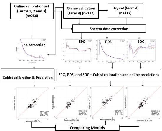
2. Materials and Methods

2.1. Study Area

The study area comprised of four farms with a total area of 105 ha at Melle (50°59′6″ N, 3°49′8″ E), Veurne (51°1′18″ N, 2°35′10″ E), Huldenberg (50°48′38″ N, 4°34′47″ E), and Landen (50°45′7″ N, 5°6′4″ E) in Flanders, Belgium (Figure 1). The study area is characterized by a temperate maritime climate with a mean annual temperature that ranged between 6 to 10 °C and annual precipitation that ranged between 750 and 1000 mm. The Melle farm included one field of about 6 ha, which was flat and elevation ranged between 4 to 5 m asl, and the soil texture varied between clay to clay loam. The Veurne farm had three fields with a total area of about 20 ha, elevation ranged between 2 to 3 m asl, and soil texture varied between clay to clay loam. This farm is affected by salinity as it is located very close to the North Sea that affects the soil with salt-water intrusion. The Huldenberg farm (35 ha) had four fields with a relatively large elevation variation of 85 to 90 m asl, and soil texture varied between sandy loam to loam. The Landen farm included three fields of about 44 ha that were almost flat except the smallest field where the elevation is higher in the middle part of the field. The texture of this farm varies between sandy loam to loam. All farms are cultivated with wheat (or barley), maize, and potato crops in rotation.

2.2. On-line Vis-NIR Measurements and Soil Sampling

An on-line spectral survey was carried out using the on-line soil sensing platform developed by Mouazen [37]. It consists of a medium-deep subsoiler, attached to a metal frame, a differential global positioning system (DGPS), and a rugged computer. The description of this sensing platform can be found in Mouazen et al. [7] and Nawar and Mouazen [9]. The spectral survey was performed using a CompactSpec mobile, fibre type, VNIR spectrophotometer (305–1700 nm) with a sampling interval of 1 nm (Tec5 Technology, Germany). A 50-watt halogen lamb was used as a light source. Light was transferred to the soil by means of a dual optical fibre, while the diffuse reflected light was collected back by the same fibre. An optical probe containing a lens holder and protected by a mild steel was appended to the back of the subsoiler chisel. The soil spectra were collected in a diffuse reflectance mode from the smoothed bottom of the trench (15–25 cm deep), made by the subsoiler itself, due to downwards vertical forces acting on the chisel. The subsoiler retrofitted optical probe was attached to a frame, which was mounted onto the three-point linkage of a tractor (Figure 2). A white Spectralon disc with about 98% reflectance was used for calibration once every 30 min. The positions of the spectra were recorded using a differential global positioning system (DGPS) (Trimble AG25, USA).
Soil spectra together with GPS data were logged through a rugged laptop computer using a standard data acquisition system. The on-line sensing for all farms was carried out using 12 m apart parallel transects and a travel speed of around 3.5 km/h. The soil scanning was carried out in summer (August to October) 2018, when the weather conditions were extremely warm and relatively dry.

2.3. Soil Samples and the Experiment

The fresh samples (381) were divided into a calibration dataset (264 samples), whose samples were collected from Huldenberg, Veurne, and Melle, and the remaining samples, collected from Landen were considered as the independent validation set (117) (Table 1). The fresh samples were mixed and reduced in size to 300 g per sample, using the quartering method. The non-soil substances such as stone/gravel, grass, roots, and other non-soil materials were manually removed. The same fresh samples of the validation set were ground, air-dried, and passed through a 2 mm sieve, after which they were scanned in the laboratory with the same spectrophotometer. Three Petri dishes of 5 cm in diameter and 2 cm deep were used for each soil sample. After the samples were placed into the dishes, the soil was levelled with a spatula to ensure a smooth surface; and therefore, maximum light reflection, and a large signal-to-noise ratio.
The SOC was determined in the laboratory using the dry combustion method, following the Dumas principle (ISO 10694; CMA/2/II/A.7; BOC). For the determination of the SOC content, total inorganic carbon (TIC) compounds were in advance removed by treating the soil samples with hydrochloric acid.

2.4. Spectra Pretreatments

The three datasets (calibration, validation, the transfer set (e.g., wet and dry)) were subjected to the same spectral pretreatment, which started with cutting the noisy part of the spectra at the two far ends, withholding the spectral range of 400–1675 nm for the spectral analysis and modeling. In the next step, the absorbance (log 1/reflectance) was calculated followed by smoothing based-on the Savitzky–Golay algorithm (providing the best predictions) [38] with a window size of 23 and a polynomial of order 2. Afterwards, the standard normal variate (snv) transformation [39] was employed to remove the baseline influences and compose spectra into a common and comparable scale, where each spectrum was normalized.
Figure 3 depicts the flow chart of steps taken during the model calibration and validation in this study. First, the fresh datasets of both the calibration and the on-line validation were treated similarly and used to calibrate and validate the Cubist model for SOC prediction without correction for SMC. The results were referred to as noncorrected prediction of SOC. Then, the three correction methods for removing SMC, namely, EPO, PDS, and OSC were used to develop the transformation matrices based-on the on-line fresh spectra and its corresponding dry samples (e.g., 117 samples). The transformation matrices had been applied then to the fresh calibration and on-line validation spectra, before the EPO-Cubist, PDS-Cubist, and OSC-Cubist models were developed and then validated. The output of these models was referred to as corrected SOC prediction. In order to evaluate the performance of the corrected models, their results were finally compared to the noncorrected Cubist model.

2.5. Algorithms to Eliminate the Effect of Soil Moisture Content from the Spectra

2.5.1. External Parameter Orthogonalization (EPO)

The concept of the EPO algorithm to eliminate the effects of external parameters is to project the spectral data onto the orthogonal to space, where changes generated by these parameter variations occur [19]. The mathematical description of EPO can be found in the literature [15,19]. In EPO, the spectra matrix X can be disintegrated into three components: a valuable component (XP) related to the chemical response, a parasitic component (XQ) that is formed by the external parameters, and N the spectral noise, as shown in Equation (1).
X = X P + X Q + N
The process is to isolate the useful component XP through the spectra matrix D, which can be calculated as the difference between the spectra matrix with external effect (on-line spectra) and without the external effect (dry spectra). P and Q are the projection matrices of the useful and parasitic components of the spectra, respectively. Q can be calculated through a singular value decomposition (SVD) of D, and the projection matrix P is then calculated from P = I − Q; I is the identity matrix. The number of EPO components g is an essential parameter that should be defined during EPO development [15,19]. This component can be determined by means of the cross-validation that resulted from PLSR on transformed spectra. In this research, the optimal value of g was defined based on the PLSR cross-validation using 1 to 6 latent variables (LVs).

2.5.2. The Piecewise Direct Standardization Algorithm (PDS)

The piecewise direct standardization (PDS) [21] is a common method to relate each wavelength in master spectra (e.g., dry spectra) and those of secondary spectra (e.g., field spectra). PDS has two advantages of using a small number of samples in the transfer set, and its multivariate nature allowing a noise-filtering effect. The transfer parameters of the PDS were determined in this study by establishing a linear relationship between the transferred samples (dry) and the corresponding on-line fresh samples (validation). The absorbance of the dry spectra measured at each wavelength was related to the wavelengths located in a predefined small window around the same wavelength measured on the on-line spectra [40]. On the on-line spectra, both of the calibration and validation sets were then standardized using the PDS parameters that allowed a direct comparison with the dry spectra. The optimal number of PLSR LVs and the size of the wavelengths window (SW) are required to apply PDS. More details about the PDS algorithm can be found in the literature [21,22]. PDS with a different size of the wavelength window (SW = 3, 5, 11, 21, 31, 41) and the optimal number of PLSR LVs (NF = 1, 2, 3, 4, 5, 6, 7, 8, 9, 10) has been tested in this work.

2.5.3. Orthogonal Signal Correction (OSC)

Orthogonal signal correction intends to correct a signal by removing information from the spectral data that is irrelevant to the targeted response variable [23]. Therefore, the spectral information orthogonal to the response variable is removed [41]. The optimal number of OSC components to be eliminated is normally defined based on PLSR cross-validation, whereas the matrices X and Y are disintegrated based on the nonlinear iterative partial least squares (NIPLS) algorithm with minimization the calibration errors criteria. The samples used to develop OSC models (the transfer set) comprise samples measured under various conditions (e.g., different moisture content), for which one aims to carry out the correction. In this work, the optimal number of OSC components to be eliminated was defined based-on the PLSR cross-validation using the maximum number of 5 LVs. The transfer samples of the dry validation set were utilized to develop the OSC models that consisted of samples measured under laboratory (dry spectra) and field (fresh on-line spectra) conditions.

2.6. Principal Component Analysis (PCA)

The principal component analysis (PCA) was used to explore the difference between the three data sets that resulted from the three corrections methods. PCA concentrates the total variation in the dataset in only a few principal components (PCs) and each obtained PC presents decreasing amounts of the variance. This analysis made possible the identification of spectral variations due to the effect of SMC, while preserving the majority of information that originated from the spectral data. The PCA similarity maps of PC1 and PC2 were used to show differences between the dry samples and the corresponding fresh samples after corrections.

2.7. Modeling with Cubist

The spectral measurements obtained during the on-line and laboratory (dry) scanning modes were used to build predictive models before and after spectral corrections with EPO, PDS, and OSC using Cubist [30]. In principle, the Cubist algorithm constructs a regression tree, where intermediate linear models provide the prediction at each step. The original data is divided by the algorithm into subsets of identical samples and develops multilinear regression rules by choosing the optimal predictor variables among all of the spectral variables to be used in the regression. These rules are connected and each rule takes a form of condition sequence: ‘’if [condition is true] then [regress rule], and else [apply the next rule]’’. If a condition is being true, then calculate the next prediction value. If not, the sequence of if, then, and else is repeated [42]. In this study, it is assumed that the Cubist algorithm is capable of recognizing the effective spectral features for constructing a robust multivariate regression model to predict SOC. Cubist available at the caret R-package [43] with the most likely two hyper-parameters (the committees and neighbors) having the largest effect on the final performance tuning of the Cubist model was used.
To evaluate the model’s performance, four parameters were used: the root mean squared error (RMSE); the coefficient of determination (R2); the ratio of performance to deviation (RPD); and the ratio of performance to the inter-quartile range (RPIQ); [44]. The spectral data processing and the modeling were performed using the R-packages: pls [45]; prospectr [46]; and caret [43].

3. Results

3.1. Spectral Data and Correction Methods

Table 2 shows the summary statistics of SOC and SMC in the calibration and the on-line prediction datasets. The SOC ranged between 0.86% and 2.40% for the calibration set and between 0.96% and 2.04% for the validation set, with median and mean values of 1.28% and 1.34% and 1.27% and 1.33%, respectively. The standard deviation (SD) values were 0.33 for the calibration set and 0.25 for the validation set. This data confirms that the range of SOC content of the validation set is smaller than that the calibration set, which is necessary to ensure the model validity for the studied range in the validation set.
SMC for the calibration set ranged between 2.28% to 24.59% with a mean and median of 12.28% and 13.03%, respectively. The SMC of the on-line validation set ranged between 11.27% and 25.03% with a mean and median of 19.40% and 20.29%, respectively. Indeed, SMC was relatively high at the time of on-line measurement (Table 2).
Figure 4 shows the spectral data of the three datasets before (Figure 4a) and after the three spectra correction methods (Figure 4b–d) for the SMC effect. The notable minor difference is observable for spectra after the EPO originated from subtracting the spectra of dry samples from the corresponding spectra of on-line fresh samples (Figure 4b), where the effect of SMC has been completely removed. In the PDS and OSC methods (Figure 4c,d, respectively), soil moisture in both cases has not been completely eliminated in particular for the OSC, where the variation between the three spectra is clear, compared to the results of EPO, and PDS to some extent.

3.2. Principal Component Space of EPO, PDS, and OSC Datasets

Figure 5 compares the principal component similarity maps of the first two principal components (PC1 and PC2), derived from the PCA carried out on the on-line calibration spectra and laboratory dry and on-line validation spectra. These components accounted for 55.3% and 35.5%, respectively, of the total variation presented in the calibration set of the uncorrected data (Figure 5a). The influence of SMC on grouping and separation of the three sets, namely, the fresh on-line calibration, the fresh on-line validation, and the dry laboratory validation spectra can be clearly observed. The separation is particularly clear for the dry validation spectra, with a minor overlap with the calibration spectra. After correcting for the effect of SMC, e.g., by applying the EPO for all the three datasets (Figure 5b), the three groups of spectra overlap now, indicating that the SMC effect has been indeed eliminated from the corrected spectra.
The projection of calibration and validation sets in PC space showed different patterns according to the correction method applied. Without correction, different convex hulls between the fresh (of both the calibration and online validation sets) and the dry (laboratory validation) sets is noticeable (Figure 6a). When projecting the fresh and dry spectra of EPO in PC space, the convex hulls of the on-line and laboratory validation sets coincided with each other, with both deviating from that of the on-line calibration set by almost 90°. The centroids of convex hulls for the on-line validation (fresh) spectra overlay with that of the laboratory dry spectra (Figure 6b), whereas the centroids of the calibration set deviated from both validation centroids. With the PDS correction, the convex hulls of the three sets coincide well, with a small deviation observed for the on-line calibration set (Figure 6c). Indeed, the centroids of convex hulls for the three datasets were almost overlaid (Figure 6c). The results of the OSC correction method were the worst, as exhibited by the deviation between the convex hulls of the three sets. Here, the centroids of convex hulls of the three datasets did not match (Figure 6d), in a similar fashion to the uncorrected spectra, as shown in (Figure 6a).

3.3. Cubist Modeling Results

3.3.1. Cubist Modeling without Spectral Correction

Table 3 and Figure 7a show that the Cubist cross-validation resulted in a good performance with RMSE, R2, RPD, and RPIQ of 0.15%, 0.74, 1.99, and 3.23, respectively. The on-line prediction yielded a less good prediction performance (RMSE = 0.20%, R2 = 0.55, RPD = 1.24, and RPIQ = 1.69).

3.3.2. Cubist Modeling after Spectral Correction

Both the cross-validation and prediction of the EPO-Cubist model outperformed both of the PDS-Cubist and OSC-Cubist models. For the cross-validation, the EPO-Cubist showed a modest improvement compared to the Cubist without spectral correction with RMSE, R2, RPD, and RPIQ of 0.11%, 0.89, 2.95, and 3.393, respectively (Table 3 and Figure 7b). The PDS showed a smaller improvement in prediction (RMSE = 0.12%, R2 = 0.87, RPD = 2.73, and RPIQ = 3.64) than that of the EPO, but a slightly better performance than that of the OSC (RMSE = 0.12%, R2 = 0.84, RPD = 2.66, and RPIQ = 3.55) (Table 3; Figure 7c,d).
The same trend of performance can be observed for the on-line prediction with the best performance obtained with the EPO (RMSE = 0.12%, R2 = 0.76, RPD = 2.08, and RPIQ = 2.83), followed successively by the PDS (RMSE = 0.14%, R2 = 0.70, RPD = 1.77, and RPIQ = 2.41) and OSC (RMSE = 0.16%, R2 = 0.67, RPD = 1.55, and RPIQ = 2.11).

3.4. Variable Importance before and after Spectra Correction

The heat map of the variable importance analysis indicates the same important variables for the developed models in the current research (Figure 8). The spectral regions at 406–436, 566–576, 656–666, 786–836, 1026–1036, 1406–1456, 1498–1536, and 1576–1606 nm are the most important bands for predicting SOC. In the VIS range, the bands of 406–436, 566–576, and 656–666 nm are located between the red absorption band (680 nm) and the blue band (450 nm) and are attributed to the electron transition associated with soil colour [47]. In the NIR range, the 786–836 band is associated with the C–H bond at 825, and the 1026–1036 band is near the absorption feature at 1035 nm, associated with the aromatic hydrocarbon (C–H) bond [26]. The band at 1406–1426 is relative to the absorption peak near the 1400 nm and that is related to the second overtone of O–H absorption at 1450 nm [48]. The bands at 1498–1536 and 1576–1606 nm are related to the first overtone of C–H, O–H, and N–H bonds [47].

4. Discussion

4.1. Soil and Spectral Data Analysis

Table 1 indicated that SD and the range of SOC are comparable for the calibration and validation sets. The concentration range or SD of the target soil property can influence the model prediction accuracy [48]. For good prediction, the range of the validation set should be within the range of the calibration set [5]. However, larger range or SD will introduce not only higher R2 and RPD, but higher RMSEP too [48]. Indeed, the narrow range of SOC of both the validation and calibration sets (0.68 to 2.40 %) influenced the prediction accuracy obtained in this study.
SMC was relatively high, particularly in the on-line validation. Consequently, the effect of SMC on spectra is potentially high. Although alterations in soil reflectance can be related to variations in SMC, SOC, and texture [49], acquisition of the on-line data can induce the spectral variability due to machine vibration, ambient light, and variation of sensor-to-soil distance and angle [7]. The effect of SMC on soil VNIR spectra has been well reported in earlier studies [15,50,51], findings that are consistent with our results. Figure 4 demonstrates that the albedo of the on-line spectrum is generally lower than that of the laboratory spectrum, although the absorption peak in the second OH overtone at 1450 nm is larger. The lower albedo of the on-line spectrum might be attributed to the illumination conditions, plant debris, and variation in the sensor-to-soil distance and inclination [52,53,54]. Therefore, the main difference noticed between the uncorrected spectra (on-line and laboratory) can be attributed to the spectral intensity and not to a spectral signature. This difference is indeed due to the different SMC and other ambient conditions encountered during on-line measurement. Therefore, it was assumed that the on-line data have sufficient quality for further spectral analysis.

4.2. The Performance of EPO, PDS, and OSC for Spectral Correction

The results of spectral correction indicating that EPO outperformed both PDS and OSC. EPO showed a high performance of removing the variation of soil absorbance that originated by moisture, since EPO has resulted in identical spectra to those of the dry sample after EPO transformation (Figure 4). The PC projection plot confirmed the best performance of EPO, as the centroids of convex hulls for the on-line validation set surrounded with the convex hulls of their corresponding dry spectra. The convex hulls of both the on-line and laboratory dry spectra coincided well over each other, with minor deviation (Figure 6). These results are in line with the findings of Chakraborty et al. [20] for EPO. Similarly, PDS was shown as a capable algorithm to correct the spectra for the moisture effect, although it performed less well compared to EPO. Examining the PC projection, a notable match between the three convex hulls can be observed with only slight deviations, which might be attributed to the noise at the two ends of the transformed spectra (Figure 4c), as PDS works with a moving window of data [22]. The poor match between the convex hulls between the laboratory dry and the on-line spectra with the on-line spectra corrected by OSC, as shown in Figure 6d, explains the poorest results of OSC in predicting SOC. In this case, the centroids of convex hulls of the three datasets dispersed without any matching tendency. This confirms that the EPO transformation has successfully corrected the spectra for the moisture effect, indicating the potential of EPO to result in the best Cubist model prediction accuracy for SOC.

4.3. Performance of Cubist Models before Moisture Correction

The predictive performance of the Cubist model without spectral correction in this research is considered poor (Table 3). A larger RMSEP of 0.31% (0.203% in the present work) was reported by Nawar and Mouazen [9] for the on-line measurement of SOC, using 529 samples combined with multivariate adaptive regression splines (MARS). Kuang and Mouazen [55] estimated SOC with a PLSR model, using a European dataset (425 soil samples) spiked with local samples that provided a similar result (RMSEP = 0.19%) to that reported in the present work. The poor prediction performance of Cubist in this research can be attributed to the effect of SMC on the VNIR spectra [51,56], which is in agreement with the literature stating that the prediction of SOC from field fresh spectra without appropriate correction is inaccurate [15,22,55]. This is indeed supported by the similarity map of PC1 and PC2 in Figure 5a, showing a clear separation between the validation and calibration sets. The laboratory spectra occupied a separate spectral space than the corresponding on-line spectra without any overlap observed. Another reason might be that the on-line spectra are influenced by other external factors (e.g., noise due to vibration, sensor-to-soil distance variation, ambient light) in addition to SMC.
In general, the variability range of SOC is a fundamental factor that affects model prediction performance [48]. Thus, with large soil heterogeneity in a target soil attribute, regression can be more successful compared with small variability. The reason for the rather poor performance of estimating SOC based-on the Cubist method in this study may be the narrow range of SOC in the calibration (1.54%) and prediction (1.08%) datasets (Table 2). However, the obtained RMSE values in the current study are not substantially higher compared with the literature, e.g., using random forest [5]. The predictive performance of the current work is of similar accuracy to that reported by Kuang and Mouazen [55] for on-line prediction of SOC at the farm-scale using the PLSR technique, with 0.12–0.96 R2 and 1.07–4.95 RPD. However, numerous studies reported similar results for SOC prediction to our results [57,58,59], with R2 values ranging from 0.55 to 0.79 and RPD from 1.80 to 2.01. The exposed large differences in the accuracy of the SOC estimates may be related to the high SOC variability and SMC effect. Although the calibration set in the present study is based-on the on-line collected spectra, that is highly affected by SMC and is of narrow variability range of SOC, prediction accuracies are reasonable, which can be attributed to the capability of Cubist to handle the nonlinearity between the SOC concentration and spectra.
The most effective bands in the VIS range were 406–436 and 656–666 nm, which are located, respectively, around the blue band (450 nm) [17] and the red band (680 nm) associated with electron transition. It is well-documented that the darker the soil color, the larger the SOC content [47]. In the NIR range, the most effective bands were 786–836, 1026–1036, 1406–1456, 1498–1536, and 1576–1606 nm. The 786–836 nm band is characterized with a broad region around 825 nm, which is associated with aromatic (C–H) and organic matter [26]. The band 956–1036 nm is associated with the third overtone of O–H (950 nm) [26]. The band 1406–1456 nm is associated with the second overtone of water absorption band around 1450 nm [7,60]. The 1498–1536, and 1576–1606 nm bands are associated with the first overtone of C–H, O–H, and N–H bonds [47], and are consequently related to the concentration of the SOC in the samples.
For SOC estimation in this work there was no rule for the best fitting of the data, and the prediction was based on the whole VNIR spectral range. It can be clearly observed in the heat map shown in Figure 8, that the NIR spectral range has contributed more to the prediction of SOC than those of the VIS spectral region. This result is in line with previous findings, e.g. [60], who reported that the NIR spectral range provided considerably better predictions of SOC than the VIS range. The prediction accuracy of SOC using the whole VNIR spectral range was better than the corresponding accuracy reported for the NIR spectral range only [7].

4.4. Performance of the Cubist Models after Correction for Moisture

The algorithms used to eliminate the effect of SMC from spectral data enhanced the performance of SOC models. EPO-Cubist yielded 40% reductions in RMSE for the on-line prediction, which is in agreement with a finding by Ackerson et al. [61], who obtained an error reduction of 63% using fresh field spectra. Ge et al. [55] using rewetted samples reported an error reduction of 60%. However, the smaller improvement of the on-line prediction of SOC achieved in this work, compared to that reported elsewhere can be attributed to the smaller difference in SMC between the on-line validation set and that of the on-line calibration set (Figure 5a). However, the correction methods, in particular EPO, provided reasonable accuracy for the on-line scanned dataset, to be recommended for future research on the on-line measurement, not only for SOC, but also on other soil properties.
The EPO-Cubist modelling found in this work as the best method to predict SOC suggests that it is not obligatory to use air-dried legacy samples for developing the calibration models, which is an important conclusion to ultimately reduce the laboratory time-consuming processing efforts. Instead, the on-line collected fresh spectra having a wide range of SMC can be used, after the correction of SMC effect to estimate SOC [60]. Both Ackerson et al. [16] and Wijewardane et al. [62] demonstrated that the utilization of EPO-based in situ spectra is essential for generating the initial EPO. Our results of EPO correction proposed that the projection matrix based-on the on-line spectra and corresponding air-dry spectra, when applied to the on-line spectral library with a varied moisture content can decrease logistical necessities by efficiently removing the effect of SMC from the spectra and, therefore, improving the prediction accuracy of SOC. The results of this research should be further tested in terms of applicability for moisture correction for the on-line prediction of other soil properties having direct or indirect spectral responses in the VNIRS spectroscopy.

5. Conclusions

This study investigated the use of the Cubist algorithm combined with spectral correction algorithms to remove the effect of soil moisture content (SMC) from on-line collected visible and near infrared (VNIR) spectra and improve the soil organic carbon (SOC) prediction accuracy of spectra collected from multiple fields in Belgium. Three correction methods, namely, external parameter orthogonalization (EPO), piecewise direct standardization (PDS), and orthogonal signal correction (OSC) were used to correct the spectral data for the removal of SMC from the on-line samples. The results showed that the EPO method outperformed both the PDS and OSC methods in eliminating the influence of differential moisture on soil VINR spectra. The EPO-Cubist model provided the best SOC prediction accuracy. It can be concluded that the use of on-line scanned spectra for developing calibration models for the prediction of SOC is possible and reliable, which reduces the effort related to preprocessing of samples in the laboratory, e.g., drying, grinding, and sieving. As EPO was found to be the best performing method, its projection matrix can be applied directly to effectively reduce the influence of SMC from the on-line spectra, supporting the sensor-based variable rate applications, and providing solutions to speed up the on-line soil mapping at field scale. Further work is suggested to test if the success obtained in the present work can be extended to other soil properties, when using the on-line data collection mode.

Author Contributions

Conceptualization and methodology, S.N. and M.A.M.; spectral measurement, M.A.M.; data analysis and modeling, S.N.; original draft preparation, S.N.; review and editing, M.A.M., S.N., and A.M.M. All authors have read and agreed to the published version of the manuscript.

Funding

This research was funded by the Research Foundation—Flanders (FWO) for the Odysseus I SiTeMan Project (No. G0F9216N).

Conflicts of Interest

The authors declare no conflict of interest.

References

  1. Hoyle, F.C.; Baldock, J.A.; Murphy, D.V. Soil Organic Carbon—Role in Rainfed Farming Systems. In Rainfed Farming Systems; Springer: Dordrecht, The Netherlands, 2011; pp. 339–361. [Google Scholar]
  2. Bresson, L.M.; Koch, C.; Le Bissonnais, Y.; Barriuso, E.; Lecomte, V. Soil Surface Structure Stabilization by Municipal Waste Compost Application. Soil Sci. Soc. Am. J. 2001, 65, 1804–1811. [Google Scholar] [CrossRef]
  3. Wang, G.; Huang, Y.; Wang, E.; Yu, Y.; Zhang, W. Modeling Soil Organic Carbon Change across Australian Wheat Growing Areas, 1960–2010. PLoS ONE 2013, 8, e63324. [Google Scholar] [CrossRef] [PubMed]
  4. Kuang, B.; Mahmood, H.S.; Quraishi, M.Z.; Hoogmoed, W.B.; Mouazen, A.M.; van Henten, E.J. Sensing Soil Properties in the Laboratory, In Situ, and On-Line. Adv. Agron. 2012, 114, 155–223. [Google Scholar]
  5. Nawar, S.; Mouazen, A.M.M. On-line vis-NIR spectroscopy prediction of soil organic carbon using machine learning. Soil Tillage Res. 2019, 190, 120–127. [Google Scholar] [CrossRef]
  6. Stenberg, B.; Viscarra Rossel, R.A.; Mouazen, A.M.; Wetterlind, J. Visible and Near Infrared Spectroscopy in Soil Science. In Advances in Agronomy; Sparks, D.L., Ed.; Academic Press: Burlington, NJ, USA, 2010; Volume 107, pp. 163–215. [Google Scholar] [CrossRef] [Green Version]
  7. Mouazen, A.M.; Maleki, M.R.; De Baerdemaeker, J.; Ramon, H. On-line measurement of some selected soil properties using a VIS-NIR sensor. Soil Tillage Res. 2007, 93, 13–27. [Google Scholar] [CrossRef]
  8. Viscarra Rossel, R.A.; Walvoort, D.J.; McBratney, A.B.; Janik, L.J.; Skjemstad, J.O. Visible, near infrared, mid infrared or combined diffuse reflectance spectroscopy for simultaneous assessment of various soil properties. Geoderma 2006, 131, 59–75. [Google Scholar] [CrossRef]
  9. Nawar, S.; Mouazen, A.M. Comparison between random forests, artificial neural networks and gradient boosted machines methods of on-line Vis-NIR spectroscopy measurements of soil total nitrogen and total carbon. Sensors 2017, 17, 2428. [Google Scholar] [CrossRef]
  10. Bricklemyer, R.S.; Brown, D.J. On-the-go VisNIR: Potential and limitations for mapping soil clay and organic carbon. Comput. Electron. Agric. 2010, 70, 209–216. [Google Scholar] [CrossRef]
  11. Christy, C.D. Real-time measurement of soil attributes using on-the-go near infrared reflectance spectroscopy. Comput. Electron. Agric. 2008, 61, 10–19. [Google Scholar] [CrossRef]
  12. Tekin, Y.; Tumsavas, Z.; Mouazen, A.M. Effect of Moisture Content on Prediction of Organic Carbon and pH Using Visible and Near-Infrared Spectroscopy. Soil Sci. Soc. Am. J. 2012, 76, 188–198. [Google Scholar] [CrossRef]
  13. Mouazen, A.M.; De Baerdemaeker, J.; Ramon, H. Effect of wavelength range on the measurement accuracy of some selected soil constituents using visual-near infrared spectroscopy. J. Near Infrared Spectrosc. 2006, 14, 189–199. [Google Scholar] [CrossRef]
  14. Bogrekci, I.; Lee, W.S. Spectral Soil Signatures and sensing Phosphorus. Biosyst. Eng. 2005, 92, 527–533. [Google Scholar] [CrossRef]
  15. Minasny, B.; Mcbratney, A.B.; Bellon-Maurel, V.; Roger, J.M.; Gobrecht, A.; Ferrand, L.; Joalland, S. Removing the effect of soil moisture from NIR diffuse reflectance spectra for the prediction of soil organic carbon. Geoderma 2011, 167–168, 118–124. [Google Scholar] [CrossRef] [Green Version]
  16. Ackerson, J.P.; Morgan, C.L.S.; Ge, Y. Penetrometer-mounted VisNIR spectroscopy: Application of EPO-PLS to in situ VisNIR spectra. Geoderma 2017, 286, 131–138. [Google Scholar] [CrossRef] [Green Version]
  17. Morgan, C.L.S.; Waiser, T.H.; Brown, D.J.; Hallmark, C.T. Simulated in situ characterization of soil organic and inorganic carbon with visible near-infrared diffuse reflectance spectroscopy. Geoderma 2009, 151, 249–256. [Google Scholar] [CrossRef]
  18. Wijewardane, N.K.; Ge, Y.; Morgan, C.L.S.S. Geoderma Moisture insensitive prediction of soil properties from VNIR reflectance spectra based on external parameter orthogonalization. Geoderma 2016, 267, 92–101. [Google Scholar] [CrossRef] [Green Version]
  19. Roger, J.M.; Chauchard, F.; Bellon-Maurel, V. EPO-PLS external parameter orthogonalisation of PLS application to temperature-independent measurement of sugar content of intact fruits. Chemom. Intell. Lab. Syst. 2003, 66, 191–204. [Google Scholar] [CrossRef] [Green Version]
  20. Chakraborty, S.; Li, B.; Weindorf, D.C.; Morgan, C.L.S. External parameter orthogonalisation of Eastern European VisNIR-DRS soil spectra. Geoderma 2019, 337, 65–75. [Google Scholar] [CrossRef]
  21. Wang, Y.; Veltkamp, D.J.; Kowalski, B.R. Multivariate Instrument Standardization. Anal. Chem. 1991, 63, 2750–2756. [Google Scholar] [CrossRef]
  22. Ji, W.; Viscarra Rossel, R.A.; Shi, Z. Accounting for the effects of water and the environment on proximally sensed vis-NIR soil spectra and their calibrations. Eur. J. Soil Sci. 2015, 66, 555–565. [Google Scholar] [CrossRef]
  23. Wold, S.; Antti, H.; Lindgren, F.; Öhman, J. Orthogonal signal correction of near-infrared spectra. Chemom. Intell. Lab. Syst. 1998, 44, 175–185. [Google Scholar] [CrossRef]
  24. Woody, N.A.; Feudale, R.N.; Myles, A.J.; Brown, S.D. Transfer of Multivariate Calibrations between Four Near-Infrared Spectrometers Using Orthogonal Signal Correction. Anal. Chem. 2004, 76, 2595–2600. [Google Scholar] [CrossRef] [PubMed]
  25. Stevens, A.; Nocita, M.; Tóth, G.; Montanarella, L.; van Wesemael, B. Prediction of Soil Organic Carbon at the European Scale by Visible and Near InfraRed Reflectance Spectroscopy. PLoS ONE 2013, 8, e66409. [Google Scholar] [CrossRef]
  26. Viscarra Rossel, R.A.; Behrens, T. Using data mining to model and interpret soil diffuse reflectance spectra. Geoderma 2010, 158, 46–54. [Google Scholar] [CrossRef]
  27. Jaconi, A.; Don, A.; Freibauer, A. Prediction of soil organic carbon at the country scale: Stratification strategies for near-infrared data. Eur. J. Soil Sci. 2017, 68, 919–929. [Google Scholar] [CrossRef]
  28. Kuang, B.; Tekin, Y.; Mouazen, A.M. Comparison between artificial neural network and partial least squares for on-line visible and near infrared spectroscopy measurement of soil organic carbon, pH and clay content. Soil Tillage Res. 2015, 146, 243–252. [Google Scholar] [CrossRef]
  29. Liu, S.; Shen, H.; Chen, S.; Zhao, X.; Biswas, A.; Jia, X.; Shi, Z.; Fang, J. Estimating forest soil organic carbon content using vis-NIR spectroscopy: Implications for large-scale soil carbon spectroscopic assessment. Geoderma 2019, 348, 37–44. [Google Scholar] [CrossRef]
  30. Quinlan, J.R. Combining Instance-Based and Model-Based Learning. In Machine Learning Proceedings 1993; Morgan Kaufmann Publishers: San Francisco, FL, USA, 2014; pp. 236–243. [Google Scholar]
  31. Appelhans, T.; Mwangomo, E.; Hardy, D.R.; Hemp, A.; Nauss, T. Evaluating machine learning approaches for the interpolation of monthly air temperature at Mt. Kilimanjaro, Tanzania. Spat. Stat. 2015, 14, 91–113. [Google Scholar] [CrossRef] [Green Version]
  32. Walton, J.T. Subpixel urban land cover estimation: Comparing cubist, random forests, and support vector regression. Photogramm. Eng. Remote Sensing 2008, 74, 1213–1222. [Google Scholar] [CrossRef] [Green Version]
  33. Sorenson, P.T.; Underwood, A.; Sorenson, P.T.; Small, C.; Tappert, M.C.; Quideau, S.A.; Drozdowski, B.; Underwood, A.; Janz, A. Monitoring organic carbon, total nitrogen and pH for field reclaimed soils using reflectance spectroscopy. Can. J. Soil Sci. 2017, 97, 241–248. [Google Scholar] [CrossRef]
  34. Peng, Y.; Xiong, X.; Adhikari, K.; Knadel, M.; Grunwald, S.; Greve, M.H. Modeling soil organic carbon at regional scale by combining multi-spectral images with laboratory spectra. PLoS ONE 2015, 10. [Google Scholar] [CrossRef] [PubMed] [Green Version]
  35. Filippi, P.; Cattle, S.R.; Bishop, T.F.A.; Jones, E.J.; Minasny, B. Combining ancillary soil data with VisNIR spectra to improve predictions of organic and inorganic carbon content of soils. MethodsX 2018, 5, 551–560. [Google Scholar] [CrossRef] [PubMed]
  36. Morellos, A.; Pantazi, X.-E.E.; Moshou, D.; Alexandridis, T.; Whetton, R.; Tziotzios, G.; Wiebensohn, J.; Bill, R.; Mouazen, A.M. Machine learning based prediction of soil total nitrogen, organic carbon and moisture content by using VIS-NIR spectroscopy. Biosyst. Eng. 2016, 152, 104–116. [Google Scholar] [CrossRef] [Green Version]
  37. Mouazen, A.M. Soil sensing device. In International publication, Published under the Patent Cooperation Treaty (PCT); World Intellectual Property Organization, International Bureau: Brussels, Belgium, International Publication Number; W02006/015463; PCT/ BE 2005/000129; IPC: G01N21/00; GO1N21/00; 2006. [Google Scholar]
  38. Savitzky, A.; Golay, M.J.E. Smoothing and Differentiation of Data by Simplified Least Squares Procedures. Anal. Chem. 1964, 36, 1627–1639. [Google Scholar] [CrossRef]
  39. Barnes, R.J.; Dhanoa, M.S.; Lister, S.J. Standard normal variate transformation and de-trending of near-infrared diffuse reflectance spectra. Appl. Spectrosc. 1989, 43, 772–777. [Google Scholar] [CrossRef]
  40. Wold, S.; Sjöström, M.; Eriksson, L. PLS-regression: A basic tool of chemometrics. Chemom. Intell. Lab. Syst. 2001, 58, 109–130. [Google Scholar] [CrossRef]
  41. Boulet, J.C.; Roger, J.M. Pretreatments by means of orthogonal projections. Chemom. Intell. Lab. Syst. 2012, 117, 61–69. [Google Scholar] [CrossRef] [Green Version]
  42. Viscarra Rossel, R.A.; Webster, R. Predicting soil properties from the Australian soil visible-near infrared spectroscopic database. Eur. J. Soil Sci. 2012, 63, 848–860. [Google Scholar] [CrossRef]
  43. Kuhn, M. Building predictive models in R using the caret package. J. Stat. Softw. 2008, 28, 1–26. [Google Scholar] [CrossRef] [Green Version]
  44. Bellon-Maurel, V.; Fernandez-Ahumada, E.; Palagos, B.; Roger, J.M.; McBratney, A. Critical review of chemometric indicators commonly used for assessing the quality of the prediction of soil attributes by NIR spectroscopy. TrAC Trends Anal. Chem. 2010, 29, 1073–1081. [Google Scholar] [CrossRef]
  45. Mevik, B.-H.; Wehrens, R.; Liland, K.H. Partial Least Squares and Principal Component Regression [R Package pls Version 2.7-1]. Available online: https://cran.r-project.org/web/packages/pls/index.html (accessed on 2 March 2020).
  46. Stevens, A.; Ramirez Lopez, L.; Lopez, L.R. Package ‘prospectr’: Miscellaneous Functions for Processing and Sample Selection of Spectroscopic Data. Available online: https://cran.r-project.org/web/packages/prospectr/prospectr.pdf (accessed on 16 March 2020).
  47. Viscarra Rossel, R.A.; Cattle, S.R.; Ortega, A.; Fouad, Y. In situ measurements of soil colour, mineral composition and clay content by vis-NIR spectroscopy. Geoderma 2009, 150, 253–266. [Google Scholar] [CrossRef]
  48. Kuang, B.; Mouazen, A.M. Calibration of visible and near infrared spectroscopy for soil analysis at the field scale on three European farms. Eur. J. Soil Sci. 2011, 62, 629–636. [Google Scholar] [CrossRef]
  49. Mouazen, A.M.; De Baerdemaeker, J.; Ramon, H.; Mounem, A.; De Baerdemaeker, J.; Ramon, H. Towards development of on-line soil moisture content sensor using a fibre-type NIR spectrophotometer. Soil Tillage Res. 2005, 80, 171–183. [Google Scholar] [CrossRef]
  50. Lobell, D.B.; Asner, G.P. Moisture Effects on Soil Reflectance. Soil Sci. Soc. Am. J. 2002, 66, 722. [Google Scholar] [CrossRef]
  51. Mouazen, A.M.; Ramon, H. Expanding implementation of an on-line measurement system of topsoil compaction in loamy sand, loam, silt loam and silt soils. Soil Tillage Res. 2009, 103, 98–104. [Google Scholar] [CrossRef] [Green Version]
  52. Poggio, M.; Brown, D.J.; Bricklemyer, R.S. Laboratory-based evaluation of optical performance for a new soil penetrometer visible and near-infrared (VisNIR) foreoptic. Comput. Electron. Agric. 2015, 115, 12–20. [Google Scholar] [CrossRef] [Green Version]
  53. Schirrmann, M.; Gebbers, R.; Kramer, E. Performance of Automated Near-Infrared Reflectance Spectrometry for Continuous in Situ Mapping of Soil Fertility at Field Scale. Vadose Zo. J. 2013, 12, 1–14. [Google Scholar] [CrossRef]
  54. Rodionov, A.; Pätzold, S.; Welp, G.; Pallares, R.C.; Damerow, L.; Amelung, W. Sensing of Soil Organic Carbon Using Visible and Near-Infrared Spectroscopy at Variable Moisture and Surface Roughness. Soil Sci. Soc. Am. J. 2014, 78, 949–957. [Google Scholar] [CrossRef]
  55. Kuang, B.; Mouazen, A.M. Effect of spiking strategy and ratio on calibration of on-line visible and near infrared soil sensor for measurement in European farms. Soil Tillage Res. 2013, 128, 125–136. [Google Scholar] [CrossRef] [Green Version]
  56. Ge, Y.; Morgan, C.L.S.; Ackerson, J.P. VisNIR spectra of dried ground soils predict properties of soils scanned moist and intact. Geoderma 2014, 221–222, 61–69. [Google Scholar] [CrossRef]
  57. Summers, D.; Lewis, M.; Ostendorf, B.; Chittleborough, D. Visible near-infrared reflectance spectroscopy as a predictive indicator of soil properties. Ecol. Indic. 2011, 11, 123–131. [Google Scholar] [CrossRef]
  58. Fontán, J.M.; Calvache, S.; López-Bellido, R.J.; López-Bellido, L. Soil carbon measurement in clods and sieved samples in a Mediterranean Vertisol by Visible and Near-Infrared Reflectance Spectroscopy. Geoderma 2010, 156, 93–98. [Google Scholar] [CrossRef]
  59. Gao, Y.; Cui, L.; Lei, B.; Zhai, Y.; Shi, T.; Wang, J.; Chen, Y.; He, H.; Wu, G. Estimating soil organic carbon content with visible-near infrared (Vis-NIR) spectroscopy. Appl. Spectrosc. 2015, 68, 712–722. [Google Scholar] [CrossRef] [PubMed]
  60. Sudduth, K.A.; Hummel, J.W. Portable, near-infrared spectrophotometer for rapid soil analysis. Trans. Am. Soc. Agric. Eng. 1993, 36, 185–194. [Google Scholar] [CrossRef]
  61. Ackerson, J.P.; Demattê, J.A.M.; Morgan, C.L.S. Predicting clay content on field-moist intact tropical soils using a dried, ground VisNIR library with external parameter orthogonalization. Geoderma 2015, 259–260, 196–204. [Google Scholar] [CrossRef]
  62. Wijewardane, N.K.; Hetrick, S.; Ackerson, J.; Morgan, C.L.S.; Ge, Y. VisNIR integrated multi-sensing penetrometer for in situ high-resolution vertical soil sensing. Soil Tillage Res. 2020, 199, 104604. [Google Scholar] [CrossRef]
Figure 1. Location map of the studied farms, namely, Melle, Veurne, Huldenberg, and Landen in Flanders, Belgium.
Remotesensing 12 01308 g001
Figure 2. The on-line visible and near infrared (vis-NIR) spectroscopy sensor developed by Mouazen [37], showing the main components (right) and the on-line spectral data acquisition (left).
Remotesensing 12 01308 g002
Figure 3. The flow chart of different steps taken in this study for soil organic carbon (SOC) prediction with the Cubist modeling approach applied on noncorrected and corrected spectra for soil moisture content (SMC) effect, using the three correction methods, namely, external parameter orthogonalization (EPO), piecewise direct standardization (PDS), and orthogonal signal correction (OSC).
Remotesensing 12 01308 g003
Figure 4. The spectral curve for mean representative spectrum in the on-line (fresh) calibration set (on-line Cal), on-line (fresh) validation set (on-line Val), and its corresponding laboratory dry set (lab dry):(a) before spectral correction (b) after external parameter orthogonalization (EPO), (c) piecewise direct standardization (PDS), and (d) orthogonal signal correction (OSC) methods.
Remotesensing 12 01308 g004
Figure 5. Score plots of principle components 1 (PC1) and 2 (PC2) of the fresh on-line (fresh) calibration (on-line Cal), dry laboratory (lab dry), and on-line (fresh) validation (on-line Val) spectra, resulted from the principal component analysis applied on (a) uncorrected spectra, and (b) corrected spectra with external parameter orthogonalization (EPO), shown as an example.
Remotesensing 12 01308 g005
Figure 6. Mean spectra from on-line (fresh) calibration set (on-line Cal), dry laboratory set (lab dry), and on-line (fresh) validation set (on-line Val) (a) before spectra correction and after spectra correction using (b) external parameter orthogonalization (EPO), (c) piecewise direct standardization (PDS), and (d) orthogonal signal correction (OSC) transformation projected on principal component 1 (PC1) vs. principal component 1 (PC2) space. The convex hulls and centroids of each dataset are represented by dashed lines and crosses, respectively.
Remotesensing 12 01308 g006
Figure 7. Scatter plots of measured soil organic carbon (SOC) versus the cross-validation (upper row of plots) and on-line prediction (lower row of plots) using Cubist models developed for (a) uncorrected (Cubist) and corrected spectra with (b) external parameter orthogonalization (EPO-Cubist), (c) piecewise direct standardization (PDS-Cubist), and (d) orthogonal signal correction (OSC-Cubist)
Remotesensing 12 01308 g007
Figure 8. Heat map of the variable importance analysis retrieved from the Cubist models built under different spectral correction schemes of uncorrected Cubist (Cubist), correct Cubist with external parameter orthogonalization (EPO-Cubist), piecewise direct standardization (PDS-Cubist), and orthogonal signal correction (OSC-Cubist).
Remotesensing 12 01308 g008
Table 1. Summary of statistical description for the soil organic carbon (SOC) and soil moisture content (SMC) for the samples collected from Huldenberg, Veurne, Melle, and Landen Farms, Belgium.
FarmProperty (%)NoMin.1QMed.Mean3QMax.SD
HuldenbergSOC1550.861.021.241.311.502.400.37
SMC1552.204.646.957.569.4019.03.25
VeurneSOC840.851.151.241.311.442.400.29
SMC8412.2916.4218.9018.6420.8824.592.80
MelleSOC251.201.501.641.611.721.900.17
SMC2511.2713.0315.0514.6415.9217.641.91
LandenSOC1170.961.151.271.331.492.040.25
SMC11711.2716.6220.2919.4021.7925.033.25
Table 2. Summary of statistical description for the soil organic carbon (SOC) and soil moisture content (SMC) for the calibration and validation datasets.
NoMin.1QMed.Mean3QMax.SD
SOC (%)Cal set (on-line fresh)2640.861.091.281.341.532.400.33
Val set (dry and on-line fresh)1170.961.151.271.331.492.040.25
SMC (%)Cal set (on-line fresh)2642.286.9213.0312.2817.0624.596.01
Val set (on-line set fresh)11711.2716.6220.2919.4021.7925.033.25
Table 3. Quality of prediction models of soil organic carbon (SOC) obtained from the Cubist modeling for uncorrected (Cubist) and corrected spectra for soil moisture content (SMC) using external parameter orthogonalization (EPO-Cubist), piecewise direct standardization (PDS-Cubist), and orthogonal signal correction (OSC-Cubist).
Cross-ValidationOn-Line Prediction
RMSER2RPDRPIQRMSEPR2RPDRPIQ
(%) (%)
Cubist0.1510.741.993.230.2030.551.241.69
EPO-Cubist0.1120.892.953.930.1200.762.082.83
PDS-Cubist0.1210.872.733.640.1410.701.772.41
OSC-Cubist0.1240.842.663.550.1610.671.552.11

