Article

Antarctic Supraglacial Lake Identification Using Landsat-8 Image Classification

by
Anna Ruth W. Halberstadt
1,*,
Colin J. Gleason
2,
Mahsa S. Moussavi
3,4,
Allen Pope
3,4,
Luke D. Trusel
5 and
Robert M. DeConto
1
1
Department of Geosciences, University of Massachusetts, Amherst, MA 01003, USA
2
Department of Civil and Environmental Engineering, University of Massachusetts, Amherst, MA 01003, USA
3
National Snow and Ice Data Center, Boulder, CO 80303, USA
4
Cooperative Institute for Research in Environmental Sciences, University of Colorado, Boulder, CO 80309, USA
5
Department of Geography, The Pennsylvania State University, University Park, PA 16801, USA
*
Author to whom correspondence should be addressed.
Remote Sens. 2020, 12(8), 1327; https://doi.org/10.3390/rs12081327
Submission received: 2 March 2020 / Revised: 15 April 2020 / Accepted: 16 April 2020 / Published: 22 April 2020
(This article belongs to the Section Environmental Remote Sensing)

Abstract

:
Surface meltwater generated on ice shelves fringing the Antarctic Ice Sheet can drive ice-shelf collapse, leading to ice sheet mass loss and contributing to global sea level rise. A quantitative assessment of supraglacial lake evolution is required to understand the influence of Antarctic surface meltwater on ice-sheet and ice-shelf stability. Cloud computing platforms have made the required remote sensing analysis computationally trivial, yet a careful evaluation of image processing techniques for pan-Antarctic lake mapping has yet to be performed. This work paves the way for automating lake identification at a continental scale throughout the satellite observational record via a thorough methodological analysis. We deploy a suite of different trained supervised classifiers to map and quantify supraglacial lake areas from multispectral Landsat-8 scenes, using training data generated via manual interpretation of the results from k-means clustering. Best results are obtained using training datasets that comprise spectrally diverse unsupervised clusters from multiple regions and that include rock and cloud shadow classes. We successfully apply our trained supervised classifiers across two ice shelves with different supraglacial lake characteristics above a threshold sun elevation of 20°, achieving classification accuracies of over 90% when compared to manually generated validation datasets. The application of our trained classifiers produces a seasonal pattern of lake evolution. Cloud shadowed areas hinder large-scale application of our classifiers, as in previous work. Our results show that caution is required before deploying ‘off the shelf’ algorithms for lake mapping in Antarctica, and suggest that careful scrutiny of training data and desired output classes is essential for accurate results. Our supervised classification technique provides an alternative and independent method of lake identification to inform the development of a continent-wide supraglacial lake mapping product.

Graphical Abstract

1. Introduction

Both the Greenland and Antarctic ice sheets are losing mass at an increasing rate (e.g., [1,2,3,4,5,6,7,8]). The Greenland Ice Sheet is projected to contribute up to ~25 cm of global mean sea level by the year 2100 under ’worst case’ greenhouse-gas emissions scenarios [9]. In contrast, mass loss from the Antarctic Ice Sheet has the potential to raise global mean sea level by tens of meters in future centuries (e.g., [10,11,12,13]) and is projected to dominate global sea level rise in the near future [14,15]. Surface meltwater plays a central role in ice sheet contributions to sea level through both direct surface meltwater runoff and indirect ice dynamical impacts. Liquid meltwater produced on the surface of an ice sheet can pool into bodies of water, such as lakes or streams, if underlain by an icy surface that is sufficiently impermeable. The influence of supraglacial hydrology on ice-sheet dynamics has been extensively explored for the Greenland Ice Sheet, where rapid drainage of surface lakes via hydrofracture to the ice-sheet bed during the early melt season and the development of perennial river networks that drain into moulins during the mid to late season influence subglacial effective pressures and ice flow velocities on short and longer timescales (e.g., [16,17,18,19,20,21,22,23,24,25,26,27,28]).
Supraglacial lakes are of particular importance in Antarctica, where their presence has been shown to induce ice-shelf collapse [29,30,31,32,33], which impacts the flow of upstream ice (e.g., [34,35,36,37,38]) and can trigger dynamic instabilities [39,40,41,42,43]. As Antarctic air temperatures increase, supraglacial lakes will become an increasingly important component of ice sheet mass balance through both direct export via drainage by surface streams [44,45] and meltwater-induced hydrofracturing that can trigger ice-shelf collapse and rapid sea-level rise due to associated dynamic acceleration of interior ice [13]. Supraglacial lakes are generally visually distinct in satellite images; dark blue lakes generally stand out against a white background of snow and ice. Individual lakes are relatively easy to identify manually, but mapping lakes reliably, repeatably, and efficiently across large spatial and temporal scales requires a systematic remote sensing approach.
Previous efforts to identify supraglacial lakes from multispectral satellite data have primarily focused on the Greenland Ice Sheet. A threshold-based approach (i.e., classifying lakes by whether or not reflectances exceed a threshold) has been successful for delineating supraglacial lakes using multispectral satellite data across multiple instruments. Varying thresholds by region have been applied to individual band reflectance values as well as the ratios between bands, such as the normalized difference water index, in order to identify supraglacial lakes (e.g., [25,46,47,48,49,50,51,52,53,54,55,56,57,58,59,60]). Another approach, dynamic band thresholding, compares the red reflectance of each pixel to the mean red value within a moving window surrounding the pixel (e.g., [61,62]). Williamson et al. [63,64] incorporate this technique into their Fully Automated Supraglacial lake Tracking (FAST) algorithm for capturing lake drainage events. A dynamic moving window approach has also been successfully applied using histograms rather than a pixel mean [65,66]. Lake boundaries can be refined by assuming a bimodal distribution of band ratios [52], and textural analysis has been used to identify supraglacial lakes based on a maximum-likelihood algorithm [67]. Finally, object-oriented classification incorporates size and shape criteria in addition to band reflectance thresholds [49].
Although Antarctic lakes are smaller and shallower than Greenland lakes [54], they can potentially exert a much larger influence on ice-sheet stability and global sea level, because most of the Antarctic Ice Sheet is marine-terminating and surrounded by large floating ice shelves (covering 1.6 million km2 [68]) that are vulnerable to hydrofracturing [29,30,31,32,33]. Antarctic supraglacial lakes have been mapped on individual ice shelves using band thresholding methods [44,54,69,70] but have only recently gained wide appreciation. Kingslake et al. [71] were the first to note widespread surface lakes across Antarctica by manually mapping meltwater features across a temporal composite of cloud-free Landsat imagery. Stokes et al. [72] also mapped lakes in East Antarctica from a composite of cloud-free Landsat imagery, and provided a minimum estimate of lake area during one month of a high-melt summer (January 2017) using a normalized difference water index threshold. Both of these spatially widespread mapping approaches employ image mosaics that merge scenes from different time periods, and therefore capture a time-integrated snapshot of lakes rather than providing detailed information about lake evolution through time. These mosaics use only imagery acquired under ideal conditions (i.e., cloud-free, high sun elevation) which is not representative of the majority of imagery available over Antarctica.
In Antarctica, a high degree of user intervention and effort (i.e., manual interpretation of images) has been required to identify and map supraglacial lakes from individual images, prohibiting broad spatial and temporal coverage. Our goals for this study are to: (1) develop a method for accurate lake identification that is broadly applicable in space and time and is robust for different ice environments; (2) assess the sensitivity of lake identification to training data and especially training classes; (3) assess the sensitivity of lake identification to classification algorithms; and (4) investigate the transferability of our classification scheme across two ice shelves. Specifically, we develop a completely automated method to identify and map lakes in Google Earth Engine, using a combination of unsupervised and supervised image classification techniques to eliminate much of the manual input required. We first run unsupervised k-means clustering, which honors the full spectral diversity present in supraglacial settings and accounts for spectral information a user cannot interpret. We then interpret this output and use these interpreted classes as training data to generate trained supervised classifiers. To our knowledge, this approach has not been previously applied. Ultimately, we exhaustively test six different combinations of training classes across two different ice shelves. We describe the process of creating this classification scheme and test the sensitivity of this method to the user’s choice of training data and classification algorithm. We compare lake areas produced by our method with lake areas produced by previously published classification algorithms and assess the spatial and temporal transferability of our classification scheme.

2. Methods

2.1. Overview and Study Area

We developed our method for two areas in East Antarctica: Amery Ice Shelf and Roi Baudouin Ice Shelf (Figure 1). Amery Ice Shelf is fed by the largest ice stream in the world (Lambert Glacier; [73]), discharging about 16% of grounded ice in East Antarctica [74]. Surface meltwater features have been documented on Amery Ice Shelf for many decades (e.g., [71,75,76,77]), and meltwater has also been observed on the surface of Roi Baudouin Ice Shelf [70,71,78].
From these study area locations, we selected 20 training scenes and 52 application scenes from the available Landsat imagery to represent a wide range of sun elevations and acquisition dates and therefore spectral characteristics (Table S1). All processing was implemented within the Google Earth Engine cloud computing platform (http://code.earthengine.google.com) using scenes collected during the austral summers of 2013–2014 to 2017–2018.
Although mapping the plethora of ice surface types is not the focus of this study, successful classification of lakes relies on accurately identifying multiple ice surface characteristics (Table 1). Much of the spectral variability on the surface of the Antarctic Ice Sheet results from spatial variability in the physical properties of the ice sheet surface. We distinguish the fast-flowing ice stream environment (“flowing ice”, transported from the continent interior out to the marine margin at velocities of many meters per year), from “firn” where snowfall gradually densifies with depth. “Blue ice” occurs where the white upper layer of snow has been removed, often scoured by wind, revealing a blueish ice surface. Instead of pooling into lakes, surface meltwater can also saturate firn to form “slush”. The delineations between these supraglacial features are sometimes difficult to interpret; slush can appear very similar to shallow lakes or to wind-scoured “blue ice” regions. Additional features imaged across the Antarctic Ice Sheet surface include rock outcrops, clouds, and cloud shadows. Our supervised classification approach was built to optimize lake identification; non-lake classes were carefully curated to avoid commission errors with lakes, but accurate classification of other environments (e.g., slush, blue ice, rocks, clouds, and cloud shadows) was not the focus of this work. Throughout this work, we evaluate only the lake class product from supervised classification.

2.2. Training Data Generation

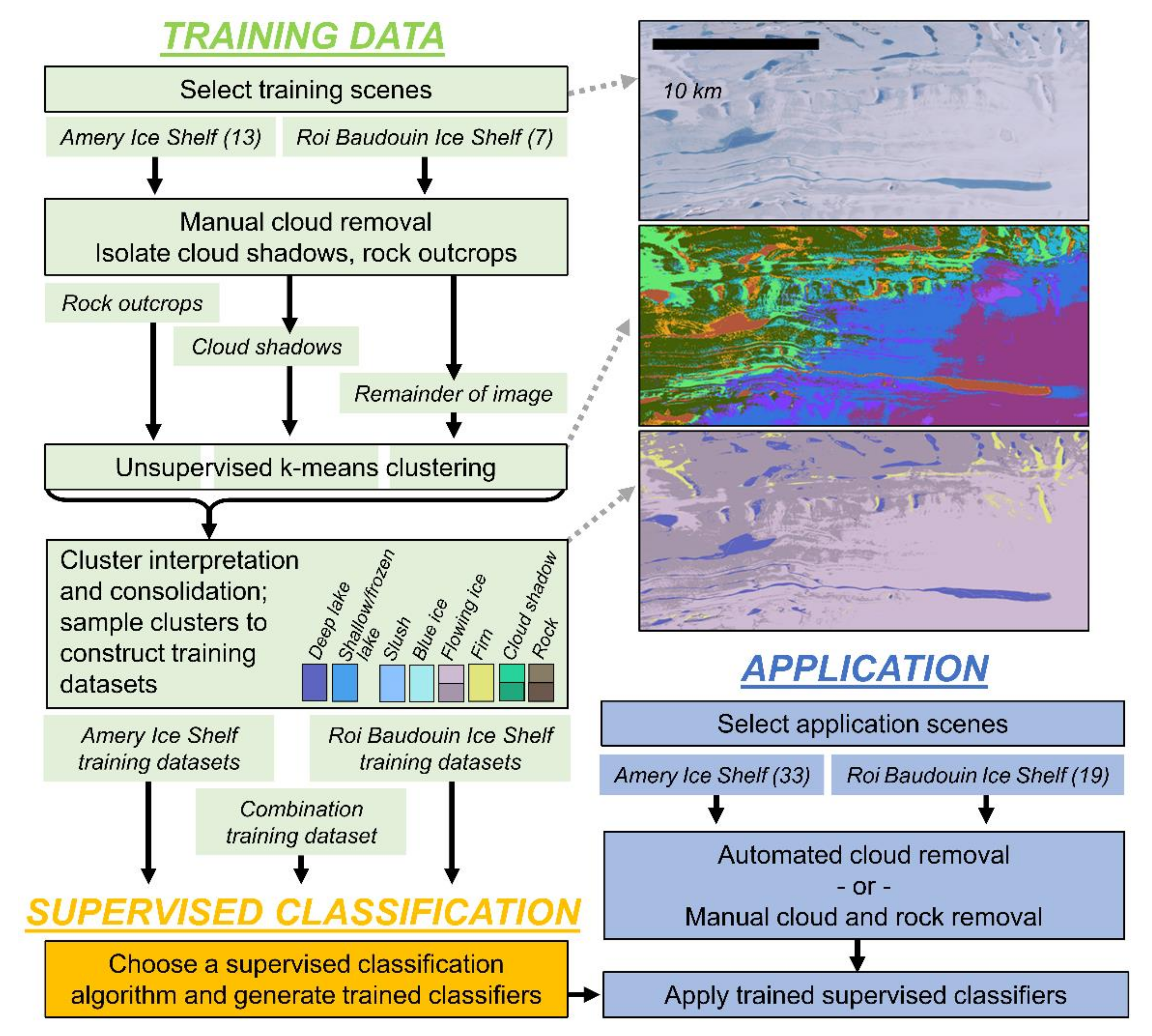
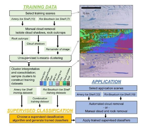
Our approach was to use an unsupervised clustering algorithm to generate statistically differentiable classes and then interpret this output as meaningful inputs into a supervised classification algorithm. Specifically, we used an unsupervised k-means clustering algorithm [80] with efficient estimation of the number of clusters [81] to first identify spectrally unique clusters. We specified a minimum and maximum number of resultant clusters (5 and 80, respectively) for the unsupervised k-means algorithm, which generally produced 30–40 unique clusters. We manually interpreted and consolidated these k-means clusters to generate specific classes of interest (Figure 2; Table 1).
Since meltwater features can be spectrally ambiguous, we tested the sensitivity of our lake mapping algorithm to different numbers of input classes. We randomly sampled 1500 pixels from each class to form training datasets (Table 1) that were named according to the number of training classes and the location of training images. An initial 6-class scheme was based on visual categorization of spectrally unique k-means clusters that represent important drivers of ice sheet process (lake, slush, blue ice, two kinds of flowing ice, firn). We observed that some k-means clusters contained pixels from very shallow lake environments along with slush pixels or non-lake pixels, so we tested splitting the ‘lake’ class into two classes (’deep lake’ and ‘shallow/frozen lake’) to form a 7-class training dataset. Liquid water pooling in lakes over an ice shelf or ice sheet can re-freeze at the lake surface (e.g., [69,82]), creating a transitional meltwater environment that has been omitted from most classification schemes [49]. We grouped these frozen lake environments into the ‘shallow/frozen lake’ training class. Two cloud shadow classes and two rock classes were added to form a 9 and 11 class training dataset, respectively; we manually mapped cloud-shadowed regions to form the cloud shadow classes, and for the rock classes, we deployed the Antarctic-wide rock mask (produced by Burton-Johnson et al. [83], accessed through the Antarctic Digital Database [https://www.add.scar.org] and buffered by 1 km to ensure complete rock coverage). Table 1 provides a summary of these training schemes.
We aim to develop an automated mapping procedure broadly applicable in space and time. Therefore, we investigate spatial transferability of supervised classifiers across both Amery and Roi Baudouin ice shelves. We supplemented the full 11-class training dataset from Amery Ice Shelf (t11A) with an additional training dataset created from Roi Baudouin Ice Shelf (t11B). A combination dataset (t11AB) contains training data from both regions (Table 1). Finally, we also explored object-based (rather than pixel-based) image analysis by constructing a training dataset that includes shape parameters (cluster area, perimeter, compactness, and elongation) in addition to the spectral properties of the individual pixels. We resampled our 11-class training dataset with this extra information about cluster shape produced through image segmentation (tOB11A and tOB11B) [84].

2.3. Supervised Classification

With our training datasets in hand, we proceeded to supervised classification (Figure 2). We generate a suite of different trained supervised classifiers by using each training dataset in Table 1 as input to a supervised classification algorithm. To develop an approach that can be easily upscaled in space and time, we used a suite of established classification algorithms accessible within the Google Earth Engine cloud computing platform. These algorithms include Random Forest, Minimum Distance, Classification and Regression Trees, Naive Bayes, Maximum Entropy, and Support Vector Machine algorithms. We then tested all possible combinations of training datasets and supervised classification algorithms (Table S3).
We compare classification results across a set of application images for both Amery and Roi Baudouin ice shelves (Figure 2). Rock outcrops were masked, and we also manually removed cloudy and cloud-shadowed regions from images prior to applying the unsupervised clustering algorithm, as these can introduce classification ambiguities. Comparing classification results across these heavily curated scenes reflects classifier performance under idealized conditions, without the confounding effect of clouds, cloud shadows and rock. However, individual scene preparation is not feasible at large spatial and temporal scales. Thus, to lay the groundwork for large-scale application of this approach, we also applied all of our 11-class supervised classifiers (including rock and cloud-shadow classes) to scenes with only automated cloud removal based on a multi-band cloud threshold developed by Moussavi et al. [85].

2.4. Validation

By necessity, classification error was quantified from limited validation data because in-situ measurements are not available for validation. We therefore constructed two validation datasets: manually mapped high-confidence lake polygons that allows us to assess only the lake/no lake areas that can be clearly interpreted visually, and a pixel-level dataset that was randomly sampled and then manually interpreted as lake or non-lake.
For the first validation dataset, we constructed high confidence lake polygons instead of a traditional shoreline trace; tracing lake outlines requires visual distinction of an often gradual transition between slush and ponded meltwater using just true-color images, a task with inherent subjective variability (e.g., [86]). Thus, we instead used only the centers of lakes to ensure that any error is due to classification and not validation data. We selected potentially ambiguous areas (slush, cloud shadow, blue ice) to comprise non-lake high-confidence polygons.
To construct our second validation dataset, we manually interpreted individual pixels. We generated 200 randomly sampled pixels within each of 6 scenes, and manually labelled each pixel as either a lake or non-lake pixel. Some of these pixels were visually ambiguous, and could not be interpreted as lake or non-lake with certainty. Instead of discarding these pixels, which would create a sampling bias in our validation dataset by disproportionately representing high confidence pixels and ignoring lake margins that are difficult to classify, we included these ambiguous pixels in the dataset with our best guess at interpretation. We report the percent of pixels with low-confidence interpretations to quantify the amount of uncertainty associated with visual interpretation.
We compared lake identification across a set of 52 application scenes: 33 over the Amery Ice Shelf and 19 over the Roi Baudouin Ice Shelf, spanning a range of sun elevation and collection dates (Table S1). The goal of this manuscript is to reliably map Antarctic lakes, so we also compared our lake identification against lakes identified through multi-band thresholding presented in companion paper Moussavi et al. [85] and previously published lake thresholds from polar regions.

3. Results

3.1. Error Assessment

We evaluate classifier accuracy against our two manually interpreted lake validation datasets: first, the high-confidence lake polygons assessing only the lake/non-lake areas that can be clearly interpreted visually; and second, the lake pixel dataset, which was randomly sampled prior to visual interpretation, representing the full variability of the scene. These validation datasets are used to assess the performance of classifiers generated from different combinations of classification algorithm and training dataset.
Many of the tested supervised classification algorithms produced high accuracies (Table S2; Table S3). When the Random Forest algorithm was used to generate supervised classifiers, those classifiers consistently produced the highest accuracies (e.g., 94.9% and 89.5% for t11AB on Amery and Roi Baudouin ice shelf validation pixels, respectively; Table S3), so we selected this algorithm as the best supervised algorithm and refer to our results using this algorithm from now on unless specified otherwise. Full description of the intercomparison of 11 classification algorithms is given in Section SI.1, which therefore achieves aim (3) of the paper. This allows us to focus on aims (1), (2), and (4), rather than tediously report differences in classification algorithm performance.
We assess the accuracy of classifiers generated from different training classes using our two validation datasets. Classifier accuracy tends to be very high when the high-confidence lake and non-lake polygons were used as the validation dataset (Table 2), demonstrating that our classification scheme is correctly identifying distinct lake and non-lake environments reliably. Manually constructed lake polygons encompass mostly deep centers of large lakes, because these environments can be more easily visually interpreted with high confidence. This presents a possible bias towards assessing accurate classification of deep lakes over shallow lakes.
For the pixel-level validation dataset, all pixels are assigned as either lake or non-lake, and we report the number of low-confidence pixels where this labeling was difficult (Table 3). Low confidence pixels range from only 3.5% to 12.0% of the total validation pixels, so we believe the overall accuracies in Table 3 are a good representation of image processing accuracy. Table 3 shows that with more training classes, classifier accuracy generally increases, although the object-based classifiers (cOB11A and cOB11B) produce lower accuracies than the pixel-based classifiers with the same training classes (c11A and c11B). Accuracy varies across the six sampled Landsat scenes in Table 3 due to differing characteristics (i.e., sun angle, cloud cover); for example, the 2016-12-26 Amery Ice Shelf scene includes more clouds and cloud shadows than the other scenes. Our classifier c11AB, generated from training data from both ice shelves, produces high accuracies over both regions.
Comparing the two validation datasets, we find that the polygon dataset produces higher accuracies than the pixel-based dataset. Mean accuracy for the polygon dataset is 98.6% (standard deviation 2.1%) for all training datasets applied to the corresponding ice shelf, while mean and standard deviation accuracy for the pixel dataset are 92.9% and 6.9%, respectively. In addition, average overall accuracy is much higher for Roi Baudouin than Amery for the pixel dataset, while the polygons show similar accuracy across both environments.

3.2. Lake Areas from Supervised Classification

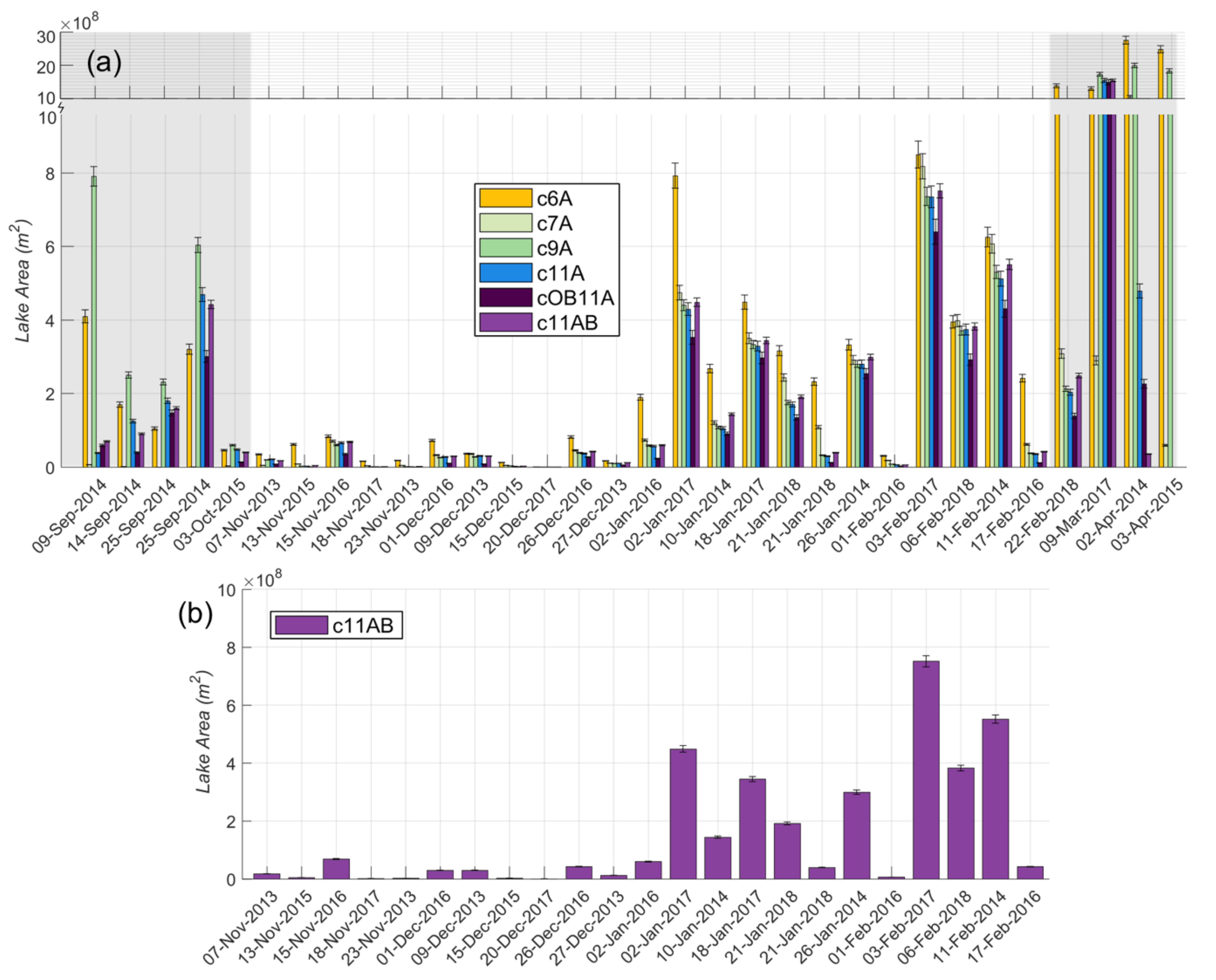
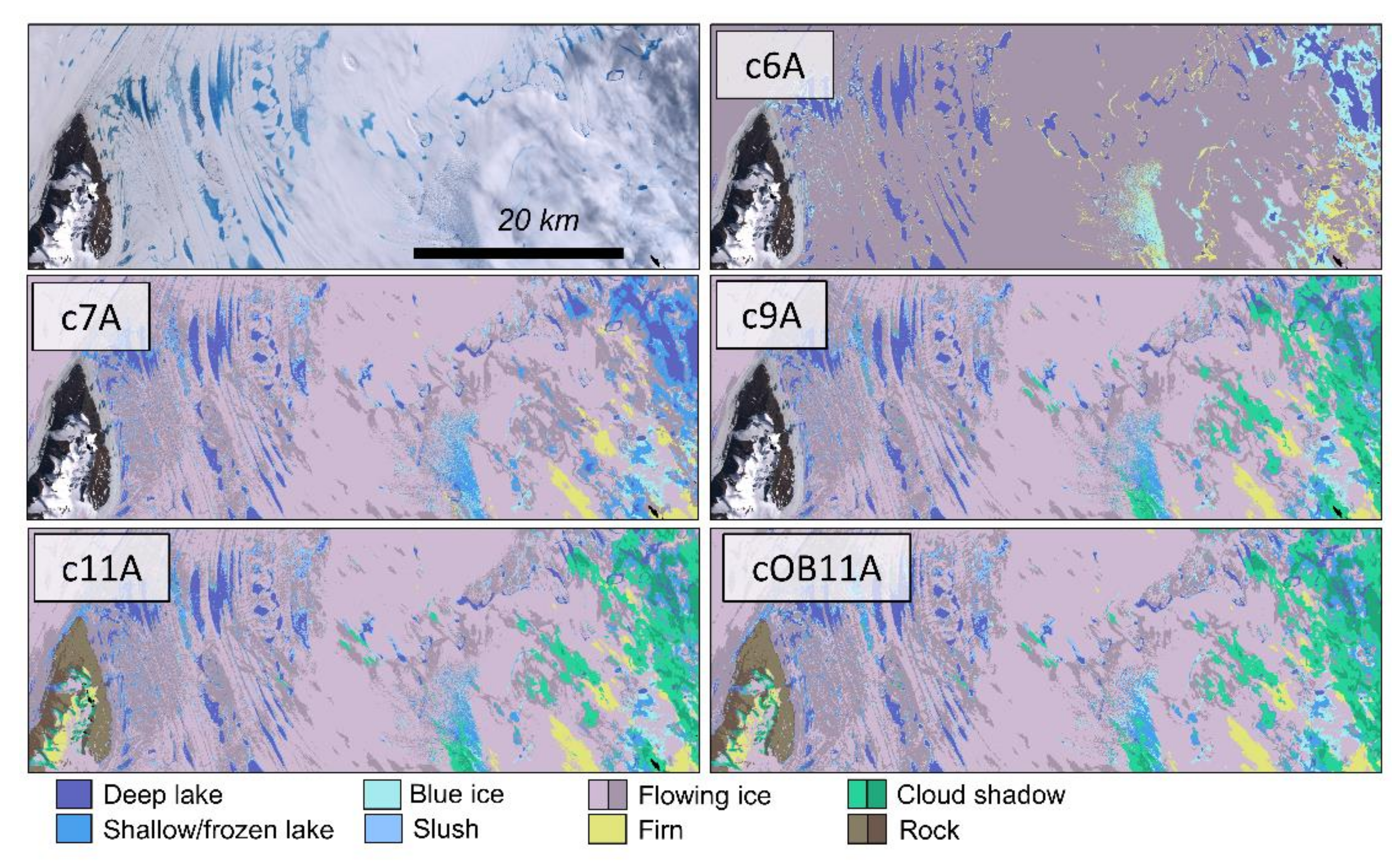
Following our stated aims, we investigated the sensitivity of classified lake areas to different choices a user could make in mapping Antarctic lakes. In addition to the supervised classification algorithm (discussed in Section SI.1.), these choices include the number of training classes and the locations of training classes. Figure 3a shows differences in lake area across training datasets for the Amery Ice Shelf application images. The initial 6-class classifier over Amery Ice Shelf (c6A: lake, slush, blue ice, two kinds of flowing ice, firn; Table 1) often misclassified large swaths of visually slushy or frozen regions as lake (Figure 4), producing relatively high lake areas (Figure 3a). With a distinction between shallow/frozen lakes and deeper lakes, the c7A classifier produced lower lake areas than c6A (Figure 3a; Figure 4). Two cloud shadow classes added to the c9A classifier led to even lower lake areas (Figure 3a; Figure 4). Figure 3a also demonstrates a strong control of sun angle on identified lake area: the shaded grey regions, denoting sun elevations < 20°, contain lake areas that vary widely across training classes or produce much larger lake areas than are physically possible. The confidence intervals on each bar in Figure 3 reveal that while each set of training data produces high-confidence lake areas, the resulting areas are sometimes quite different.
Throughout the melt season, all classifiers produced a consistent lake evolution pattern: a gradual increase in lake area, peaking during the late season, which matches the melt pattern observed at Larsen Ice Shelf [32]. Early melt season scenes (e.g., November and December) recorded zero or very low lake areas; scenes with a small number of identified lakes often captured a few meltwater ponds, or small amounts of cloud shadow misclassification. Classifiers generated from different training datasets diverged in their ability to classify low-sun-elevation scenes; with increasing number of training classes, lake area decreased for these scenes although significant misclassification remains. We obtained the lowest amount of misclassification for low-sun-elevation scenes by combining training data from both Amery and Roi Baudouin Ice Shelf (c11AB; Figure 3b).
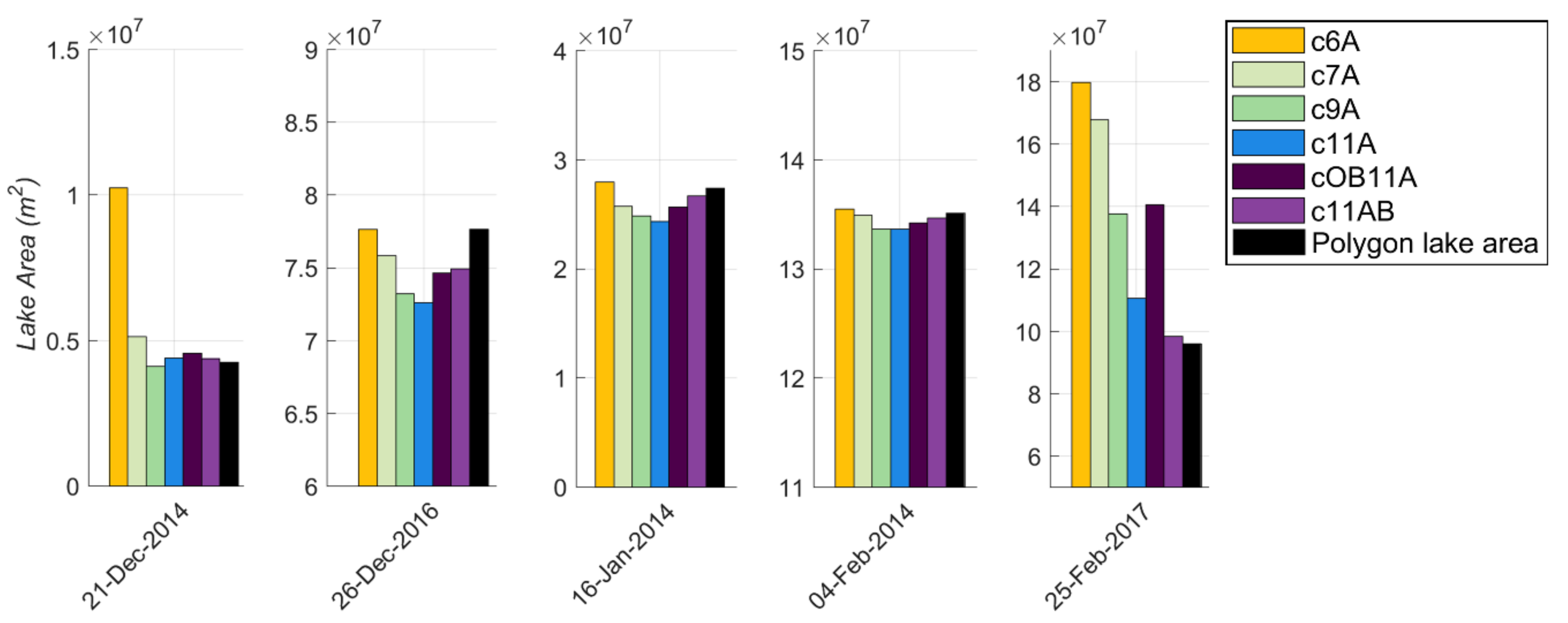
Figure 3 shows total lake area across entire scenes, but we are also interested in a more controlled experiment. Thus, we calculate lake area across all our validation polygons, applying each classifier only within the bounds of these high-confidence lake/non-lake areas to test the effect of training data on lake area calculation. In theory, a correct classification should have the same lake area as our manual lake polygons. Figure 5 compares the summed area of our lake polygons with results from supervised classifiers applied to both lake/non-lake polygons. Two date-specific patterns emerge: a pattern where classifiers match lake area better as more classes are added (21 Dec 2014, 25 Feb 2017) and a pattern where the results are relatively insensitive to the number of training classes (26 Dec 2016, 16 Jan 2014, 04 Feb 2014). Total lake area difference across training data ranged from 8.4 x 10⁷ m2 (87% percent of true area) in 25 Feb 2017 to 0.2 x 10⁷ m2 (1% percent of true area) on 04 Feb 2014.
We also investigated adding object-based classification to our supervised classification scheme. With shape parameters added as training classes, cOB11A produced lower lake areas compared to the otherwise identical pixel-based c11A classifier (Figure 3a) [Note: higher lake areas from cOB11A in the 25 Feb 2017 scene shown in Figure 5 represent cloud shadow commission error]. With object-based classification, image segmentation creates coherent lake regions, ensuring that large numbers of isolated lake pixels do not artificially inflate the calculated lake areas, but it misses some detailed lake patterns evident in the ‘noisy’ pixel-by-pixel classification (Figure 6).

3.3. Classification Transferability across Ice Shelves

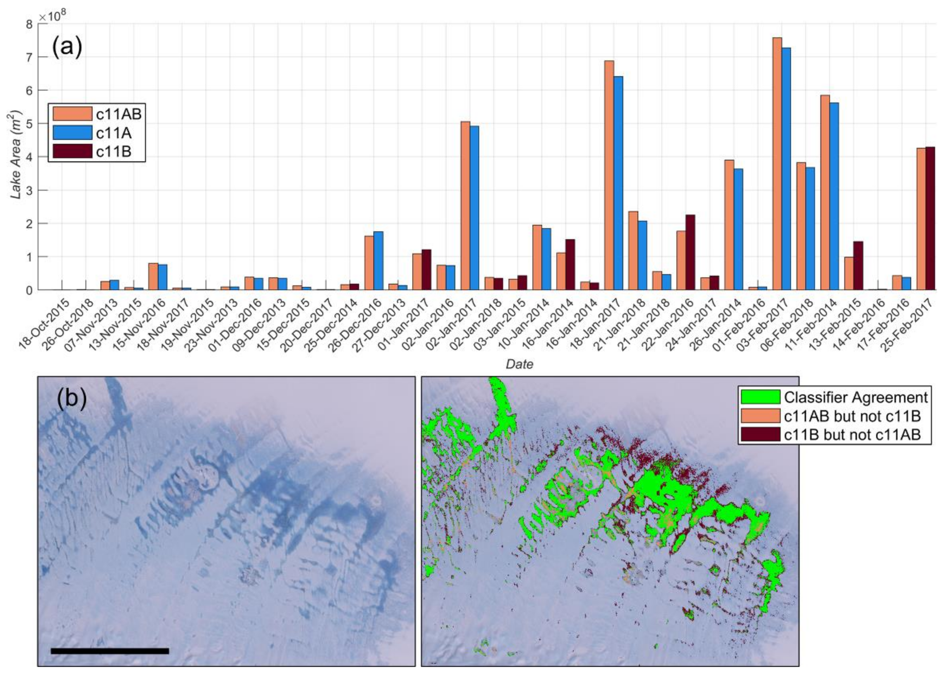
An aim of this paper is to investigate the transferability of our classification scheme across ice shelf locations. Lakes on Amery Ice Shelf are deeper and larger than on Roi Baudouin Ice Shelf, and this physical difference is important to classify correctly. First we compare a classifier generated from Amery Ice Shelf training data (c11A) with a classifier generated from Roi Baudouin Ice Shelf data (c11B) and a combination classifier generated from both regions (c11AB), by applying these classifiers to both Amery and Roi Baudouin Ice Shelf application images (Figure 7a). We observe that the combination classifier (c11AB) produces similar lake areas to both regionally trained classifiers with the same number of training classes (c11A or c11B; Figure 7a). On Roi Baudouin Ice Shelf, c11B identifies more shallow lake extents than c11AB (Figure 7b), although both capture deep lake environments.
Second, we investigate the spatial transferability of supervised classifiers by using training data from one ice shelf as validation data for the other (which renders them independent from one another; for example, a c6A trained classifier was generated from the t6A training dataset and is therefore independent from the t9B training dataset; Table 4 Classifiers generated from Amery Ice Shelf training datasets are relatively unsuccessful when applied to a dataset of interpreted pixels sampled from Roi Baudouin Ice Shelf (i.e., our Roi Baudouin training data), and vice versa. When faced with a combination 11-class dataset containing pixels from both regions, the best-performing regional classifiers (c11A from Amery and c11B from Roi Baudouin) only achieved accuracies of 78% and 66%, respectively. Conversely, the combination classifier c11AB was able to correctly classify the 11-class training datasets from both regions with an accuracy of at least 99%.

4. Discussion

4.1. Sensitivity of Lake Area Results to User Choices and Training Data

We are ultimately interested in accurate supraglacial lake mapping. Our results indicate that seemingly trivial user choices can have significant impacts on calculated lake areas, which, in turn, could lead to erroneous scientific conclusions. Our experiment design has made the effect of each of these choices explicitly clear. Principally, the number of training classes significantly impacts the lake areas identified by trained supervised classifiers (Figure 3a; Figure 4), and more accurate lake areas are obtained by distinguishing deep lakes from shallow or frozen lakes (Figure 5). The addition of cloud shadow classes further improves accuracy of the classifiers; Figure 4 demonstrates how the addition of cloud shadow classes can decrease lake misclassification (commission error). Calculated lake area is relatively insensitive to classification algorithm; similar lake areas are produced across a handful of the best-performing algorithms (Figure S1), although we use Random Forest exclusively throughout this study. Elucidating these impacts required the extensive investigation that we provide here, and would not be apparent if we had selected an ‘off the shelf’ classification method and proceeded without further analysis.
Our approach separates shallow/frozen lakes and deep lakes into different training classes (Table 1), using only the deep lake class to calculate lake area. This approach increases confidence in (deep) lake area calculations but possibly introduces omission errors for shallow lakes. Thus, the user decision regarding what constitutes a ‘lake’ can lead to significant classified lake area discrepancies. This is clear in Figure 3a, where the use of different training classes led to widely different lake areas despite the relatively high accuracy of each classifier (Table 2, Table 3). In other words, our classifiers are accurately detecting what they have been trained to detect, but they may not have been trained to classify the same lake environment. This is especially important in areas with mostly shallow lakes, such as the Roi Baudouin Ice Shelf. Furthermore, the inclusion of frozen or partially frozen lakes can significantly impact meltwater volume calculations. The definition of when ‘slushy’ or ‘shallow/frozen lake’ pixels become ‘deep lake’ pixels has implications for the wider community use of a lake mapping product and should be explicit in a final product.
Our results also show that classifiers generated from training datasets that contain only one lake class (c6A, c6B) can produce lake areas that are much too large (see c6A in Figure 3a), despite generally high classification accuracy (Table 2, Table 3). Thus, classification accuracy by itself can be misleading; high accuracy may not reflect improved understanding of the supraglacial environment, as in this example the high image classification accuracy would have badly misrepresented lake area. We assert that training classes must therefore be curated to best capture the desired lake environment, but this does not mean that adding more classes is always desirable. We argue that there are diminishing returns on addition of further classes; we have split rocks, cloud shadows, and flowing ice into two sub-classes each, but further division of classes blurs their statistical differentiability. Future work should explicitly seek to determine if there is an optimal number of classes for pan-Antarctic study.
The object-based classifier is less accurate compared to the pixel-by-pixel classifier. We hypothesize that our addition of shape parameters reduces classifier accuracy by placing less emphasis on reflectance differences. The four shape parameters we incorporate (area; perimeter; the ratio of area to perimeter; and ratio of width to height) are not unique to lake clusters; many other glacial features exhibit similar shapes as lakes (e.g., patches of blue ice, snow, and cloud shadows). Furthermore, c11A/c11B/c11AB omission error is low for high-confidence lake polygons, suggesting that pixel-based classification is already producing coherent lake areas without the extra step of image segmentation. The success of object-based classification relies on the image segmentation methodology. The initial spacing for image segmentation is set at 5 pixels, and superpixel clusters ‘grow’ from the seeded locations [84]. This spacing is comparable to the minimum lake size for the pixel-based classification method; there is no size threshold for pixel-based classification, but lakes are generally comprised of more than one pixel. The size and clustering method for creating polygons during image segmentation may significantly impact object-based classification results, but further exploration is beyond the scope of this work. As Google Earth Engine tools continue to improve, future incorporation of supervised image classification should explore more sophisticated object-based image analysis as part of the training data production and supervised classification process. Object-based classification provides a valuable minimum estimate of lake area, which could form an important baseline when upscaling lake identification spatially and temporally across Antarctica.

4.2. Spatial and Temporal Upscaling

In this work, we investigated the wider spatial and temporal application of our classification method. We tested the spatial robustness of our classification method by comparing classifier performance across Amery and Roi Baudouin ice shelves. The regional classifier generated from only Roi Baudouin scenes (c11B) is less susceptible to shadow misclassification than the regional Amery classifier (c11A) but misses a few deep lake areas. By incorporating training data from both locations, the combination classifier (c11AB) may underestimate lake area by ignoring some shallower lakes (Figure 7b) but ensures that deeper lakes are included. Combining training datasets leads to better performance for low-sun-elevation scenes (c11AB in Figure 3a) and improves classifier accuracy for cloudy scenes (e.g., scene 2016-12-26 in Table 3).
Across both ice shelves, the combination classifier c11AB performed similarly to the regionally trained classifiers c11A and c11B (Figure 7a) with generally similar accuracy despite the differences in lake characteristics (Table 2; Table 3). Cross-validation of trained classifiers with training datasets for both Amery and Roi Baudouin ice shelves (Table 4) reveals that regionally trained classifiers perform poorly when applied to another ice shelf, but the combination classifier c11AB is accurate across both regions. These observations support the assertion that spatially integrated training data produces more robust lake area identifications. This is encouraging for broad spatial application, as we would otherwise expect that regionally trained classifiers would outperform a multi-region training set. Because c11AB performs well, we have confidence for future broader training data generation.
Removing scenes with sun elevations less than 20° prevents early-season cloud shadow misclassifications. This produces a consistent seasonal lake evolution pattern, evident across both Amery and Roi Baudouin ice shelves (Figure 3, Figure 7a). However, this sun elevation filter can also remove high-melt late-season scenes from analysis, which may be problematic for capturing the full seasonal evolution of surface meltwater. Adding training data from more locations may continue to improve a classifier’s ability to correctly identify lakes in low-sun-elevation scenes. Alternatively, we could envision adding a specific ‘low angle’ set of classes to be applied only during low angle scenes. This partition into two datasets (based on image date) might allow lakes to be mapped reliably throughout the season but requires difficult analysis of early season scenes to generate training data. To continue to successfully upscale across the Antarctic continent, classification techniques will need to be applicable across more variable environments, not only encompassing different lake characteristics but also regions of extensive dirty ice and different rock outcrop lithologies.

4.3. Comparison with Threshold-Based Lake Identification

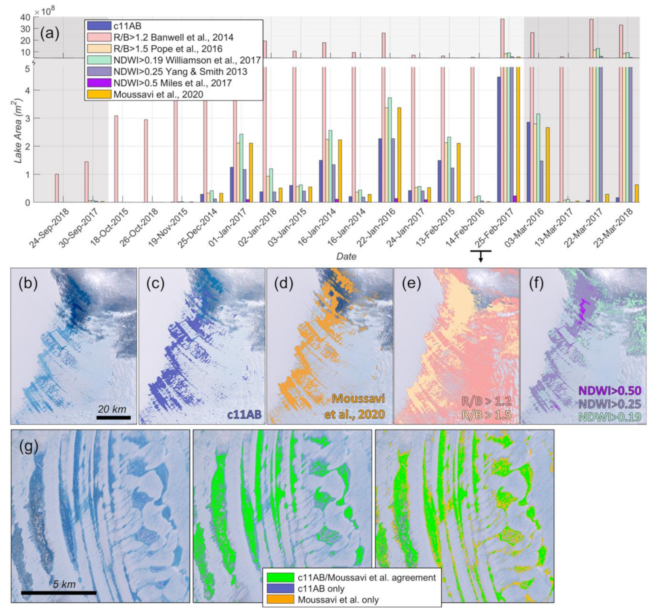
We compare our 11-class supervised classifier (c11AB) lake results to a suite of previously published spectral thresholding algorithms that have been developed for specific glacial regions on the Antarctic or Greenland Ice Sheet. These methods work by selecting single band or multi-band index thresholds to differentiate lakes. These methods are computationally efficient and easily applied at massive scale, and form a status quo in Antarctic lake mapping. Some of the spectral thresholding methods produce roughly similar lake areas as the supervised classifiers developed here, while others diverge significantly (Figure 8), which is unsurprising given the diversity in lake characteristics across polar regions and the different regions of intended application. The advent of Google Earth Engine has enabled our more computationally intensive methods to be used on the same data volumes as these threshold methods. It is not our intent to explicitly compare and evaluate these methods; rather, we highlight the widely varying lake areas that result from applying different ‘off-the-shelf’ classifiers, adding weight to our assertion that a careful treatment of supraglacial training data is crucial for the correct identification of lake area.
We compare our lake results to the multi-band spectral lake identification thresholds developed by Moussavi et al. [85] (Table 2; Table 3; Figure 8). Both methods calculate similar lake areas throughout the melt season and produce a consistent pattern of lake evolution across the melt season (Figure 8a). General similarity of lake areas calculated by the two methods confirms that the spectral signature of lakes established through our supervised classification method is independently consistent with the multi-band spectral thresholds manually derived in Moussavi et al. [85]. The Moussavi et al. [85] spectral thresholds capture more shallow or partially frozen lake environments than our supervised classifier (Figure 8g). The manually interpreted validation datasets (Table 2; Table 3) reveal that our 11-class supervised classifier c11AB is more accurate than multi-band-thresholded lakes [85] for three of the four Amery scenes (lower c11AB accuracy is achieved across the cloudiest Amery scene, 2016-12-26, due to cloud shadow commission error). Both methods used together provide critical information about the range of possible lake areas.

4.4. Classification of Non-Lake Environments and Commission Error

4.4.1. Rock Outcrops

Sunlit rock outcrops emerging from snow- and ice-covered regions have distinct spectral characteristics, but shaded rocks can appear similar to lakes. For many of the application scenes presented here, rock outcrops have been clipped out using the static rock mask. This approach ensures complete rock removal but may omit meltwater generated around exposed rock. Also, rock areas may fluctuate annually as snow cover changes over time, so a flexible rock classification is valuable. The incorporation of two rock classes in our training dataset eliminates the need to use a static rock mask on Landsat scenes prior to classification.
We investigate possible classifier confusion between lakes and shaded rocks by comparing our 9-class and 11-class supervised classifier results (c9A and c11A). We find that c9A and c11A produce very similar lake area calculations when a rock mask is applied (Figure S2), verifying that the c11A classifier does not misclassify deep lakes as rocks; similarly, resubstitution accuracy of the c11A classifier produces virtually zero commission/omission error between rock classes and lake classes. The difference between lake areas classified by c11A with and without the rock mask (Figure S2) reveals the presence of lakes near rock outcrops that are clipped out by the 1-km rock buffering procedure. The successful incorporation of rock classes into our supervised classification scheme suggests that static rock masking is not a necessary procedure for producing consistent supervised lake area classifications.

4.4.2. Cloud Shadows

Especially at low sun elevations, clouds project shadows onto ice that can be mistaken for lakes. We find that scenes with cloud shadows can have significant classification errors. The inclusion of two unique cloud shadow training classes (and two rock training classes) improve these errors but do not eliminate them (for example, Figure S3). Classification error is generally via commission, where shadowed areas are mistakenly identified as lakes. The addition of two cloud shadow classes improves commission error; classifiers with cloud shadow classes (c9A and c11A) correctly calculate smaller lake areas than without explicit cloud shadow classes, although some cloud shadowed regions are still misclassified as lakes (e.g., Figure S3).
Our pixel validation dataset highlights the difficulty of classifying lakes that are visible but shadowed by clouds; the 12-26-2016 Amery Landsat scene (Table 3) is characterized by clouds and cloud shadows, leading to relatively lower accuracies in Table 2 and Table 3. Even the 9- and 11-class supervised classifiers, with cloud shadow training classes, are only able to capture some of the lake areas that appear to underlie cloud shadow. Generally, the confounding effect of cloud shadow can lead to both omission as well as commission errors by our trained supervised classifiers. Supervised classifiers can also be confounded by lake areas shadowed by clouds, because these regions are characterized by both lake and cloud shadow environments. Trained supervised classifiers generally split these areas as partially lake and partially cloud shadow, because a pixel can only belong to one class. Cloud shadow commission error remains an obstacle to large-scale application of supervised classification techniques; best results are achieved through user intervention with careful scene selection and post-classification quality control.

5. Conclusions

Mapping the extent and evolution of surface meltwater is crucial for understanding the role of supraglacial hydrology in Antarctic ice-sheet stability, and it provides important boundary conditions for assessing the stability of the Antarctic Ice Sheet. Our goals for this manuscript were to: (1) present a method for accurate lake identification that is broadly applicable in space and time and is robust for different ice environments; (2) assess the sensitivity of lake identification to training data and training classes; (3) assess the sensitivity of lake identification to classification algorithms; and (4) explore the transferability of our classification scheme across two ice shelf locations. In this work, we developed a method that interprets unsupervised clustering to generate training data for a scalable supervised classification. We extensively iterated our approach across numerous supervised classification algorithms and training datasets to provide a complete analysis of Antarctic lake classification.
We draw the following principle conclusions. For scenes collected with sun elevation greater than 20°, accurate supervised classification of lakes is demonstrated across multiple training datasets and classification algorithms using our method. Although misclassification of cloud shadows remains a hindrance to large-scale application of supervised classifiers, our trained classifiers achieve lake/non-lake classification accuracies of over 90% based on manual lake validation datasets. We show that trained supervised classifiers can be applied across two ice shelf environments and produce a coherent melt season signal in lake area (Amery and Roi Baudouin Ice Shelves), despite differences in lake characteristics across the two regions. We also tested the sensitivity of our classification method to the choice of training dataset and classification algorithm. We found that the best classification is achieved using training datasets that distinguish deep lakes from shallow/frozen lake environments and includes unique training classes for cloud shadows. The Random Forest classification algorithm performed best, although lake area results are similar for other high-performing algorithms. This work represents a successful step towards building supervised classifiers that can be fully upscaled across the Antarctic Ice Sheet. Our method is computationally feasible at large scales and can be easily ported across the entire continent within the Google Earth Engine platform. These results provide a valuable comparison point for informing and cross-validating other methods of lake identification, ultimately geared towards creating and improving Antarctic-wide continental lake maps of surface meltwater evolution throughout the satellite observational record.

Supplementary Materials

The following are available online at https://www.mdpi.com/2072-4292/12/8/1327/s1, Table S1: Landsat product ID and sun elevation for training and application scenes, Section SI.1. Supervised Classification Algorithms, Table S2: Resubstitution accuracy for supervised classifiers using different classification algorithms, Table S3: Validation accuracy for all combinations of training dataset and supervised classification algorithm, Figure S1: Comparison of best-performing supervised classification algorithms across the set of Amery Ice Shelf application scenes, Figure S2: Comparison of rock masking versus classification using rock training classes, Figure S3: Supervised classifiers generated from different numbers of training classes applied to an Amery Ice Shelf scene.

Author Contributions

Initial conceptualization, A.R.W.H. and C.J.G; methodology and investigation, A.R.W.H., M.S.M., A.P., L.D.T., C.J.G.; resources and discussion, R.M.D.; writing—original draft preparation, A.R.W.H.; writing—review and editing, all authors. All authors have read and agreed to the published version of the manuscript.

Funding

AP and MM were funded by NSF GEO Grant 1643715. LDT was funded by NSF GEO Grant 1643733. Publication of this article was partially funded by grant 80NSSC17K0698 to the NASA Sea Level Science Team, and by the National Snow and Ice Data Center, Cooperative Institute for Research in Environmental Sciences, University of Colorado Boulder.

Acknowledgments

We thank two anonymous reviewers and Ian Willis for their thoughtful comments to improve this manuscript.

Conflicts of Interest

The authors declare no conflict of interest.

References

  1. Shepherd, A.; Ivins, E.R.; Geruo, A.; Barletta, V.R.; Bentley, M.J.; Bettadpur, S.; Briggs, K.H.; Bromwich, D.H.; Forsberg, R.; Galin, N.; et al. A reconciled estimate of ice-sheet mass balance. Science 2012, 338, 1183–1189. [Google Scholar] [CrossRef] [Green Version]
  2. Rignot, E.; Mouginot, J.; Scheuchl, B.; van den Broeke, M.; Van Wessem, M.J.; Morlighem, M. Four decades of Antarctic Ice Sheet mass balance from 1979–2017. Proc. Natl. Acad. Sci. USA 2019, 116, 1095–1103. [Google Scholar] [CrossRef] [Green Version]
  3. Harig, C.; Simons, F.J. Mapping Greenland’s mass loss in space and time. Proc. Natl. Acad. Sci. USA 2012, 109, 19934–19937. [Google Scholar] [CrossRef] [Green Version]
  4. Vaughan, D.G.; Comiso, J.; Allison, I.; Carrasco, J.; Kaser, G.; Kwok, R.; Mote, P.; Murray, T.; Paul, F.; Ren, J. Climate Change 2013: The Physical Science Basis; Contribution of Working Group I to the Fifth Assessment Report of the Intergovernmental Panel on Climate Change; Cambridge University Press: Cambridge, UK, 2013. [Google Scholar]
  5. Velicogna, I.; Sutterley, T.C.; Van Den Broeke, M.R. Regional acceleration in ice mass loss from Greenland and Antarctica using GRACE time-variable gravity data. J. Geophys. Res. Sp. Phys. 2014, 41, 8130–8137. [Google Scholar] [CrossRef] [Green Version]
  6. Van Den Broeke, M.R.; Enderlin, E.M.; Howat, I.M.; Kuipers Munneke, P.; Noël, B.P.Y.; Jan Van De Berg, W.; Van Meijgaard, E.; Wouters, B. On the recent contribution of the Greenland ice sheet to sea level change. Cryosphere 2016, 10, 1933–1946. [Google Scholar] [CrossRef] [Green Version]
  7. Noël, B.; Jan Van De Berg, W.; MacHguth, H.; Lhermitte, S.; Howat, I.; Fettweis, X.; Van Den Broeke, M.R. A daily, 1 km resolution data set of downscaled Greenland ice sheet surface mass balance (1958-2015). Cryosphere 2016, 10, 2361–2377. [Google Scholar] [CrossRef] [Green Version]
  8. Mouginot, J.; Rignot, E.; Bjørk, A.A.; van den Broeke, M.; Millan, R.; Morlighem, M.; Noël, B.; Scheuchl, B.; Wood, M. Forty-six years of Greenland Ice Sheet mass balance from 1972 to 2018. Proc. Natl. Acad. Sci. USA 2019, 116, 9239–9244. [Google Scholar] [CrossRef] [Green Version]
  9. Church, J.A.; Clark, P.U.; Cazenave, A.; Gregory, J.M.; Jevrejeva, S.; Levermann, A.; Merrifield, M.A.; Milne, G.A.; Nerem, R.S.; Nunn, P.D. Sea Level Change. Climate Change 2013: The Physical Science Basis; Contribution of working group I to the fifth assessment report of the intergovernmental panel on climate change; Cambridge University Press: Cambridge, UK, 2013; pp. 1137–1216. [Google Scholar]
  10. Winkelmann, R.; Levermann, A.; Ridgwell, A.; Caldeira, K. Combustion of available fossil fuel resources sufficient to eliminate the Antarctic Ice Sheet. Sci. Adv. 2015, 1, e1500589. [Google Scholar] [CrossRef] [Green Version]
  11. Clark, P.U.; Shakun, J.D.; Marcott, S.A.; Mix, A.C.; Eby, M.; Kulp, S.; Levermann, A.; Milne, G.A.; Pfister, P.L.; Santer, B.D.; et al. Consequences of twenty-first-century policy for multi-millennial climate and sea-level change. Nat. Clim. Chang. 2016, 6, 360–369. [Google Scholar] [CrossRef]
  12. Golledge, N.R.; Kowalewski, D.E.; Naish, T.R.; Levy, R.H.; Fogwill, C.J.; Gasson, E.G.W. The multi-millennial Antarctic commitment to future sea-level rise. Nature 2015, 526, 421–425. [Google Scholar] [CrossRef]
  13. Deconto, R.M.; Pollard, D. Contribution of Antarctica to past and future sea-level rise. Nature 2016, 531, 591–597. [Google Scholar] [CrossRef]
  14. Kopp, R.E.; Horton, R.M.; Little, C.M.; Mitrovica, J.X.; Oppenheimer, M.; Rasmussen, D.J.; Strauss, B.H.; Tebaldi, C. Probabilistic 21st and 22nd century sea-level projections at a global network of tide-gauge sites. Earth’s Futur. 2014, 2, 383–406. [Google Scholar] [CrossRef]
  15. Kopp, R.E.; DeConto, R.M.; Bader, D.A.; Hay, C.C.; Horton, R.M.; Kulp, S.; Oppenheimer, M.; Pollard, D.; Strauss, B.H. Evolving Understanding of Antarctic Ice-Sheet Physics and Ambiguity in Probabilistic Sea-Level Projections. Earth’s Futur. 2017, 5, 1217–1233. [Google Scholar] [CrossRef] [Green Version]
  16. Zwally, H.J.; Abdalati, W.; Herring, T.; Larson, K.; Saba, J.; Steffen, K. Surface Melt-Induced Acceleration of Greenland Ice-Sheet Flow. Science 2002, 297, 218–222. [Google Scholar] [CrossRef]
  17. Shepherd, A.; Hubbard, A.; Nienow, P.; King, M.; McMillan, M.; Joughin, I. Greenland ice sheet motion coupled with daily melting in late summer. Geophys. Res. Lett. 2009, 36, 2–5. [Google Scholar] [CrossRef] [Green Version]
  18. Bartholomew, I.; Nienow, P.; Mair, D.; Hubbard, A.; King, M.A.; Sole, A. Seasonal evolution of subglacial drainage and acceleration in a Greenland outlet glacier. Nat. Geosci. 2010, 3, 408–411. [Google Scholar] [CrossRef]
  19. Bartholomew, I.; Nienow, P.; Sole, A.; Mair, D.; Cowton, T.; King, M.A. Short-term variability in Greenland Ice Sheet motion forced by time-varying meltwater drainage: Implications for the relationship between subglacial drainage system behavior and ice velocity. J. Geophys. Res. Earth Surf. 2012, 117, F03002. [Google Scholar] [CrossRef]
  20. Schoof, C. Ice-sheet acceleration driven by melt supply variability. Nature 2010, 468, 803–806. [Google Scholar] [CrossRef]
  21. Sundal, A.V.; Shepherd, A.; Nienow, P.; Hanna, E.; Palmer, S.; Huybrechts, P. Melt-induced speed-up of Greenland ice sheet offset by efficient subglacial drainage. Nature 2011, 469, 521–524. [Google Scholar] [CrossRef]
  22. Hoffman, M.J.; Catania, G.A.; Neumann, T.A.; Andrews, L.C.; Rumrill, J.A. Links between acceleration, melting, and supraglacial lake drainage of the western Greenland Ice Sheet. J. Geophys. Res. Earth Surf. 2011, 116, 1–16. [Google Scholar] [CrossRef] [Green Version]
  23. Joughin, I.; Das, S.B.; Flowers, G.E.; Behn, M.D.; Alley, R.B.; King, M.A.; Smith, B.E.; Bamber, J.L.; Van Den Broeke, M.R.; Van Angelen, J.H. Influence of ice-sheet geometry and supraglacial lakes on seasonal ice-flow variability. Cryosphere 2013, 7, 1185–1192. [Google Scholar] [CrossRef] [Green Version]
  24. Chu, V.W. Greenland ice sheet hydrology: A review. Prog. Phys. Geogr. 2014, 38, 19–54. [Google Scholar] [CrossRef]
  25. Smith, L.C.; Chu, V.W.; Yang, K.; Gleason, C.J.; Pitcher, L.H.; Rennermalm, A.K.; Legleiter, C.J.; Behar, A.E.; Overstreet, B.T.; Moustafa, S.E.; et al. Efficient meltwater drainage through supraglacial streams and rivers on the southwest Greenland ice sheet. Proc. Natl. Acad. Sci. USA 2015, 112, 1001–1006. [Google Scholar] [CrossRef] [PubMed] [Green Version]
  26. Das, S.B.; Joughin, I.; Behn, M.D.; Howat, I.M.; King, M.A.; Lizarralde, D.; Bhatia, M.P. Fracture Propagation to the Base of the Greenland Ice Sheet During Supraglacial Lake Drainage. Science 2008, 320, 778–782. [Google Scholar] [CrossRef] [PubMed] [Green Version]
  27. Tedesco, M.; Willis, I.C.; Hoffman, M.J.; Banwell, A.F.; Alexander, P.; Arnold, N.S. Ice dynamic response to two modes of surface lake drainage on the Greenland ice sheet. Environ. Res. Lett. 2013, 8, 034007. [Google Scholar] [CrossRef]
  28. Doyle, S.H.; Hubbard, A.; Fitzpatrick, A.A.W.; van As, D.; Mikkelsen, A.B.; Pettersson, R.; Hubbard, B. Persistent flow acceleration within the interior of the Greenland ice sheet. Geophys. Res. Lett. 2014, 41, 899–905. [Google Scholar] [CrossRef] [Green Version]
  29. Scambos, T.; Hulbe, C.; Fahnestock, M.; Bohlander, J. The Link between Climate Warming and Ice Shelf Breakups in the Antarctic Peninsula. J. Glaciol. 2000, 46, 516–530. [Google Scholar] [CrossRef] [Green Version]
  30. Scambos, T.; Hulbe, C.; Fahnestock, M. Climate-induced ice shelf disintegration in the Antarctic Peninsula. Antarct. Penins. Clim. Var. Hist. Paleoenviron. Perspect. Antarct. Res. Ser. 2003, 79, 79–92. [Google Scholar]
  31. Banwell, A.F.; MacAyeal, D.R.; Sergienko, O.V. Breakup of the Larsen B Ice Shelf triggered by chain reaction drainage of supraglacial lakes. Geophys. Res. Lett. 2013, 40, 5872–5876. [Google Scholar] [CrossRef] [Green Version]
  32. Van den Broeke, M. Strong surface melting preceded collapse of Antarctic Peninsula ice shelf. Geophys. Res. Lett. 2005, 32, 1–4. [Google Scholar] [CrossRef] [Green Version]
  33. Sergienko, O.; Macayeal, D.R. Surface melting on Larsen Ice Shelf, Antarctica. Ann. Glaciol. 2005, 40, 215–218. [Google Scholar] [CrossRef] [Green Version]
  34. Rignot, E.; Casassa, G.; Gogineni, P.; Krabill, W.; Rivera, A.; Thomas, R. Accelerated ice discharge from the Antarctic Peninsula following the collapse of Larsen B ice shelf. Geophys. Res. Lett. 2004, 31, 2–5. [Google Scholar] [CrossRef] [Green Version]
  35. Scambos, T.A.; Bohlander, J.A.; Shuman, C.A.; Skvarca, P. Glacier acceleration and thinning after ice shelf collapse in the Larsen B embayment, Antarctica. Geophys. Res. Lett. 2004, 31, 2001–2004. [Google Scholar] [CrossRef] [Green Version]
  36. Shuman, C.A.; Berthier, E.; Scambos, T.A. 2001–2009 elevation and mass losses in the Larsen A and B embayments, Antarctic Peninsula. J. Glaciol. 2011, 57, 737–754. [Google Scholar] [CrossRef] [Green Version]
  37. Glasser, N.F.; Scambos, T.A.; Bohlander, J.; Truffer, M.; Pettit, E.; Davies, B.J. From ice-shelf tributary to tidewater glacier: Continued rapid recession, acceleration and thinning of Röhss Glacier following the 1995 collapse of the Prince Gustav Ice Shelf, Antarctic Peninsula. J. Glaciol. 2011, 57, 397–406. [Google Scholar] [CrossRef] [Green Version]
  38. Rott, H.; Müller, F.; Nagler, T.; Floricioiu, D. The imbalance of glaciers after disintegration of Larsen-B ice shelf, Antarctic Peninsula. Cryosphere 2011, 5, 125–134. [Google Scholar] [CrossRef] [Green Version]
  39. Weertman, J. Stability of the Junction of an Ice Sheet and an Ice Shelf. J. Glaciol. 1974, 13, 3–11. [Google Scholar] [CrossRef] [Green Version]
  40. Schoof, C. Ice sheet grounding line dynamics: Steady states, stability, and hysteresis. J. Geophys. Res. Earth Surf. 2007, 112, 1–19. [Google Scholar] [CrossRef] [Green Version]
  41. Bassis, J.N.; Walker, C.C. Upper and lower limits on the stability of calving glaciers from the yield strength envelope of ice. Proc. R. Soc. A Math. Phys. Eng. Sci. 2012, 468, 913–931. [Google Scholar] [CrossRef]
  42. Pollard, D.; DeConto, R.M.; Alley, R.B. Potential Antarctic Ice Sheet retreat driven by hydrofracturing and ice cliff failure. Earth Planet. Sci. Lett. 2015, 412, 112–121. [Google Scholar] [CrossRef] [Green Version]
  43. Robel, A.A.; Banwell, A.F. A Speed Limit on Ice Shelf Collapse Through Hydrofracture. Geophys. Res. Lett. 2019, 46, 12092–12100. [Google Scholar] [CrossRef] [Green Version]
  44. Bell, R.E.; Chu, W.; Kingslake, J.; Das, I.; Tedesco, M.; Tinto, K.J.; Zappa, C.J.; Frezzotti, M.; Boghosian, A.; Lee, W.S. Antarctic ice shelf potentially stabilized by export of meltwater in surface river. Nature 2017, 544, 344–348. [Google Scholar] [CrossRef] [PubMed]
  45. Bell, R.E.; Banwell, A.F.; Trusel, L.D.; Kingslake, J. Antarctic surface hydrology and impacts on ice-sheet mass balance. Nat. Clim. Chang. 2018, 8, 1044–1052. [Google Scholar] [CrossRef]
  46. Xu, H. Modification of normalised difference water index ( NDWI ) to enhance open water features in remotely sensed imagery. Int. J. Remote Sens. 2006, 27, 3025–3033. [Google Scholar] [CrossRef]
  47. Box, J.E.; Ski, K. Remote sounding of Greenland supraglacial melt lakes: Implications for subglacial hydraulics. J. Glaciol. 2007, 53, 257–265. [Google Scholar] [CrossRef] [Green Version]
  48. Doyle, S.H.; Hubbard, A.L.; Dow, C.F.; Jones, G.A.; Fitzpatrick, A.; Gusmeroli, A.; Kulessa, B.; Lindback, K.; Pettersson, R.; Box, J.E. Ice tectonic deformation during the rapid in situ drainage of a supraglacial lake on the Greenland Ice Sheet. Cryosphere 2013, 7, 129–140. [Google Scholar] [CrossRef] [Green Version]
  49. Johansson, A.M.; Brown, I.A. Adaptive classification of supra-glacial lakes on the west greenland ice sheet. IEEE J. Sel. Top. Appl. Earth Obs. Remote Sens. 2013, 6, 1998–2007. [Google Scholar] [CrossRef]
  50. Leeson, A.A.; Shepherd, A.; Sundal, A.V.; Johansson, A.M.; Selmes, N.; Briggs, K.; Hogg, A.E.; Fettweis, X. A comparison of supraglacial lake observations derived from MODIS imagery at the western margin of the Greenland ice sheet. J. Glaciol. 2013, 59, 1179–1188. [Google Scholar] [CrossRef] [Green Version]
  51. Morriss, B.F.; Hawley, R.L.; Chipman, J.W.; Andrews, L.C.; Catania, G.A.; Hoffman, M.J.; Lüthi, M.P. A ten-year record of supraglacial lake evolution and rapid drainage in West Greenland using an automated processing algorithm for multispectral imagery. Cryosphere 2013, 7, 1869–1877. [Google Scholar] [CrossRef] [Green Version]
  52. Yang, K.; Smith, L.C. Supraglacial streams on the Greenland Ice Sheet delineated from combined spectral—Shape information in high-resolution satellite imagery. IEEE Geosci. Remote Sens. Lett. 2013, 10, 801–805. [Google Scholar] [CrossRef]
  53. Arnold, N.S.; Banwell, A.F.; Willis, I.C. High-resolution modelling of the seasonal evolution of surface water storage on the Greenland Ice Sheet. Cryosphere 2014, 8, 1149–1160. [Google Scholar] [CrossRef] [Green Version]
  54. Banwell, A.F.; Caballero, M.; Arnold, N.S.; Glasser, N.F.; Cathles, L.M.; MacAyeal, D.R. Supraglacial lakes on the Larsen B ice shelf, Antarctica, and at Paakitsoq, West Greenland: A comparative study. Ann. Glaciol. 2014, 55, 1–8. [Google Scholar] [CrossRef] [Green Version]
  55. Fitzpatrick, A.A.W.; Hubbard, A.L.; Box, J.E.; Quincey, D.J.; Van As, D.; Mikkelsen, A.P.B.; Doyle, S.H.; Dow, C.F.; Hasholt, B.; Jones, G.A. A decade (2002–2012) of supraglacial lake volume estimates across Russell Glacier, West Greenland. Cryosphere 2014, 8, 107–121. [Google Scholar] [CrossRef] [Green Version]
  56. Moussavi, M.S.; Abdalati, W.; Pope, A.; Scambos, T.; Tedesco, M.; MacFerrin, M.; Grigsby, S. Derivation and validation of supraglacial lake volumes on the Greenland Ice Sheet from high-resolution satellite imagery. Remote Sens. Environ. 2016, 183, 294–303. [Google Scholar] [CrossRef] [Green Version]
  57. Pope, A. Reproducibly estimating and evaluating supraglacial lake depth with Landsat 8 and other multispectral sensors. Earth Sp. Sci. 2016, 3, 176–188. [Google Scholar] [CrossRef]
  58. Pope, A.; Scambos, T.A.; Moussavi, M.; Tedesco, M.; Willis, M.; Shean, D.; Grigsby, S. Estimating supraglacial lake depth in West Greenland using Landsat 8 and comparison with other multispectral methods. Cryosphere 2016, 10, 15–27. [Google Scholar] [CrossRef] [Green Version]
  59. Miles, K.E.; Willis, I.C.; Benedek, C.L.; Williamson, A.G.; Tedesco, M. Toward Monitoring Surface and Subsurface Lakes on the Greenland Ice Sheet Using Sentinel-1 SAR and Landsat-8 OLI Imagery. Front. Earth Sci. 2017, 5, 1–17. [Google Scholar] [CrossRef] [Green Version]
  60. Sundal, A.V.; Shepherd, A.; Nienow, P.; Hanna, E.; Palmer, S.; Huybrechts, P. Evolution of supra-glacial lakes across the Greenland Ice Sheet. Remote Sens. Environ. 2009, 113, 2164–2171. [Google Scholar] [CrossRef]
  61. Selmes, N.; Murray, T.; James, T.D. Fast draining lakes on the Greenland Ice Sheet. Geophys. Res. Lett. 2011, 38, 1–5. [Google Scholar] [CrossRef]
  62. Everett, A.; Murray, T.; Selmes, N.; Rutt, I.C.C.; Luckman, A.; James, T.D.D.; Clason, C.; Leary, M.O.; Karunarathna, H.; Moloney, V.; et al. Annual down-glacier drainage of lakes and water-filled crevasses at Helheim Glacier, southeast Greenland. J. Geophys. Res. Earth Surf. 2016, 121, 1819–1833. [Google Scholar] [CrossRef] [Green Version]
  63. Williamson, A.G.; Arnold, N.S.; Banwell, A.F.; Willis, I.C. A Fully Automated Supraglacial lake area and volume Tracking (“FAST”) algorithm: Development and application using MODIS imagery of West Greenland. Remote Sens. Environ. 2017, 196, 113–133. [Google Scholar] [CrossRef]
  64. Williamson, A.; Willis, I.C.; Arnold, N.S.; Banwell, A.F. Controls on rapid supraglacial lake drainage in West Greenland: An Exploratory Data Analysis approach. J. Glaciol. 2018, 64, 208–226. [Google Scholar] [CrossRef] [Green Version]
  65. Liang, Y.; Colgan, W.; Lv, Q.; Steffen, K.; Abdalati, W.; Stroeve, J.; Gallaher, D.; Bayou, N. A decadal investigation of supraglacial lakes in West Greenland using a fully automatic detection and tracking algorithm. Remote Sens. Environ. 2012, 123, 127–138. [Google Scholar] [CrossRef] [Green Version]
  66. Howat, I.M.; de la Peña, S.; van Angelen, J.H.; Lenaerts, J.T.M.; van den Broeke, M.R. Expansion of meltwater lakes on the Greenland Ice Sheet. Cryosphere 2013, 7, 201–204. [Google Scholar] [CrossRef] [Green Version]
  67. Lettang, F.J.; Crocker, R.I.; Emery, W.J.; Maslanik, J.A. Estimating the extent of drained supraglacial lakes on the Greenland Ice Sheet. Int. J. Remote Sens. 2013, 34, 4754–4768. [Google Scholar] [CrossRef]
  68. Depoorter, M.A.; Bamber, J.L.; Griggs, J.A.; Lenaerts, J.T.M.; Ligtenberg, S.R.M.; Van Den Broeke, M.R.; Moholdt, G. Calving fluxes and basal melt rates of Antarctic ice shelves. Nature 2013, 502, 89–92. [Google Scholar] [CrossRef]
  69. Langley, E.S.; Leeson, A.A.; Stokes, C.R.; Jamieson, S.S.R. Seasonal evolution of supraglacial lakes on an East Antarctic outlet glacier. Geophys. Res. Lett. 2016, 43, 8563–8571. [Google Scholar] [CrossRef]
  70. Lenaerts, J.T.M.; Lhermitte, S.; Drews, R.; Ligtenberg, S.R.M.; Berger, S.; Helm, V.; Smeets, C.J.P.P.; Broeke, M.R.; Van De Berg, W.J.; Van Meijgaard, E.; et al. Meltwater produced by wind-albedo interaction stored in an East Antarctic ice shelf. Nat. Clim. Chang. 2017, 7, 58–62. [Google Scholar] [CrossRef] [Green Version]
  71. Kingslake, J.; Ely, J.C.; Das, I.; Bell, R.E. Widespread movement of meltwater onto and across Antarctic ice shelves. Nature 2017, 544, 349–352. [Google Scholar] [CrossRef] [Green Version]
  72. Stokes, C.R.; Sanderson, J.E.; Miles, B.W.; Jamieson, S.S.; Leeson, A.A. Widespread development of supraglacial lakes around the margin of the East Antarctic Ice Sheet. Sci. Rep. 2019, 9, 13823. [Google Scholar] [CrossRef] [Green Version]
  73. Rignot, E.; Thomas, R.H. Mass balance of polar ice sheets. Science 2002, 297, 1502–1506. [Google Scholar] [CrossRef] [Green Version]
  74. Fricker, H.A.; Hyland, G.; Coleman, R.; Young, N.W. Digital elevation models for the Lambert Glacier-Amery ice shelf system, East Antarctica, From ERS-1 satellite radar altimetry. J. Glaciol. 2000, 46, 553–570. [Google Scholar] [CrossRef] [Green Version]
  75. Mellor, M.; McKinnon, G. The Amery Ice Shelf and its hinterland. Polar Rec. Gr. Brit. 1960, 10, 30–34. [Google Scholar] [CrossRef]
  76. Swithinbank, C. Satellite Image Atlas of Glaciers of of the World: Antarctica; U.S. Geological Survey Professional Paper 1386–B; Unites States Government Printing Office: Washington, DC, USA, 1988; Volume 1386, ISBN 2330-7102. [Google Scholar]
  77. Phillips, H.A. Surface meltstreams on the Amery Ice Shelf, East Antarctica. Ann. Glaciol. 1998, 27, 177–181. [Google Scholar] [CrossRef] [Green Version]
  78. Trusel, L.D.; Frey, K.E.; Das, S.B.; Munneke, P.K.; Van Den Broeke, M.R. Satellite-based estimates of Antarctic surface meltwater fluxes. Geophys. Res. Lett. 2013, 40, 6148–6153. [Google Scholar] [CrossRef] [Green Version]
  79. Bindschadler, R.; Vornberger, P.; Fleming, A.; Fox, A.; Mullins, J.; Binnie, D.; Paulsen, S.J.; Granneman, B.; Gorodetzky, D. The Landsat Image Mosaic of Antarctica. Remote Sens. Environ. 2008, 112, 4214–4226. [Google Scholar] [CrossRef]
  80. Arthur, D.; Vassilvitskii, S. k-means++: The advantages of careful seeding. In Proceedings of the The Eighteenth Annual ACM-SIAM Symposium on Discrete Algorithms, New Orleans, Louisiana, 7–9 January 2007; Society for Industrial and Applied Mathematics: Philadelphia, PA, USA, 2007; pp. 1027–1035. [Google Scholar]
  81. Pelleg, D.; Moore, A.W. X-means: Extending k-means with efficient estimation of the number of clusters. In Proceedings of the Seventeenth International Conference on Machine Learning (ICML 2000), Stanford, CA, USA, 29 June–2 July 2000; pp. 727–734. [Google Scholar]
  82. Hubbard, B.; Luckman, A.; Ashmore, D.W.; Bevan, S.; Kulessa, B.; Kuipers Munneke, P.; Philippe, M.; Jansen, D.; Booth, A.; Sevestre, H.; et al. Massive subsurface ice formed by refreezing of ice-shelf melt ponds. Nat. Commun. 2016, 7, 11897. [Google Scholar] [CrossRef] [Green Version]
  83. Burton-Johnson, A.; Black, M.; Peter, T.F.; Kaluza-Gilbert, J. An automated methodology for differentiating rock from snow, clouds and sea in Antarctica from Landsat 8 imagery: A new rock outcrop map and area estimation for the entire Antarctic continent. Cryosphere 2016, 10, 1665–1677. [Google Scholar] [CrossRef] [Green Version]
  84. Achanta, R.; Susstrunk, S. Superpixels and Polygons using Simple Non-Iterative Clustering. In Proceedings of the 2017 IEEE Conference on Computer Vision and Pattern Recognition (CVPR), Honolulu, HI, USA, 21–26 July 2017; pp. 4895–4904. [Google Scholar]
  85. Moussavi, M.S.; Pope, A.; Halberstadt, A.R.W.; Trusel, L.D.; Cioffi, L.; Abdalati, W. Antarctic supraglacial lake detection using Landsat 8 and Sentinel-2 imagery: Towards continental generation of lake volumes. Remote Sens. 2020, 12, 134. [Google Scholar] [CrossRef] [Green Version]
  86. Paul, F.; Barrand, N.E.; Baumann, S.; Berthier, E.; Bolch, T.; Casey, K.; Frey, H.; Joshi, S.P.; Konovalov, V.; Le Bris, R.; et al. On the accuracy of glacier outlines derived from remote-sensing data. Ann. Glaciol. 2013, 54, 171–182. [Google Scholar] [CrossRef] [Green Version]
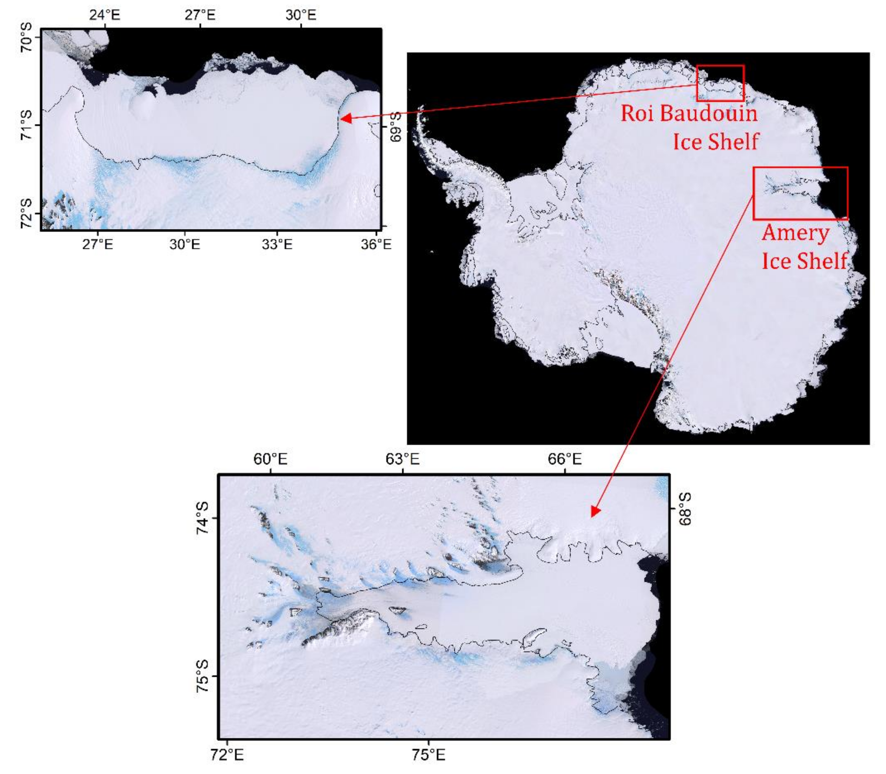
Figure 1. Amery Ice Shelf and Roi Baudouin Ice Shelf locations, with the grounding line (separating floating and grounded ice) shown in black. Imagery is from the Landsat Image Mosaic of Antarctica [79].
Remotesensing 12 01327 g001
Figure 2. Schematic workflow for creating training data (green), generating trained supervised classifiers (orange) and applying the classifiers over Amery and Roi Baudouin ice shelves (blue). Landsat product ID and sun elevation for each training and application scene used in this study are provided in Table S1. An example of the training process is shown for scene LC08_L1GT_128111_20140211. In this example we show results from an 11-class training dataset, although we test numerous training datasets with different training classes in this study (Table 1). In this scene subset, only 4 of the 11 classes are depicted (‘Deep lake’, two types of ’Flowing ice’, and ‘Firn’).
Remotesensing 12 01327 g002
Figure 3. Lake areas are identified across a set of application scenes across the Amery Ice Shelf, categorized by date of image acquisition. Classifiers were generated from different training datasets. Manual cloud/cloud shadow polygons and the rock mask were applied prior to classification. (a) Grey shading indicates scenes with sun elevation below 20°. Note the upper scale is compressed to show the exceedingly high (misclassified) lake areas for some low-sun-elevation scenes. Error bars reflect the validation accuracy of each classifier (Table 3). (b) c11AB classifier results with low-sun-elevation scenes removed. For the final scene (April 3, 2015) the c11A, cOB11A, and c11AB classifiers produced zero lake area.
Remotesensing 12 01327 g003
Figure 4. Results for different trained classifiers (described in Table 1), applied to scene LC08_L1GT_128111_20170118. A rock mask was applied prior to classification when using the c6A, c7A, and c9A classifiers but not for c11A or cOB11A.
Remotesensing 12 01327 g004
Figure 5. For the five scenes with manual high-confidence lake/non-lake polygons, we compare the sum of the lake polygon areas with classified lake areas results across both lake and non-lake polygon areas.
Remotesensing 12 01327 g005
Figure 6. A subset of Landsat scene LC08_L1GT_127111_20140204 is shown in true color (a), alongside results from pixel-based (b) and object-based (c) classifiers.
Remotesensing 12 01327 g006
Figure 7. (a) Classified lake areas from c11A, c11B, and c11AB classifiers applied to both Amery Ice Shelf and Roi Baudouin Ice Shelf. Scenes were filtered to remove imagery with sun elevations less than 20°. (b) An example of classifier difference is shown across shallow lakes on the Roi Baudouin Ice Shelf (scene LC08_L1GT_153109_20160303).
Remotesensing 12 01327 g007
Figure 8. (a) Comparison of our supervised classifier with published band thresholding methods developed for other polar regions, applied to Roi Baudouin Ice Shelf application scenes following automated cloud removal. Grey shading indicates scenes with sun elevation below 20°. Note the upper scale is compressed to show the exceedingly high (misclassified) lake areas for some low-sun-elevation scenes. (b) The true-color image shows a subset of scene LC08_L1GT_154109_20170225 with enhanced contrast to highlight lakes partially visible beneath cloud shadows. Lakes identified by our c11AB classifier (c) are compared to previously published lake identification methods based to the ratio of red to blue reflectance: (d) multi-band thresholding by Moussavi et al. [85]; (e) Red/blue (‘R/B’) thresholds from Banwell et al. [54] for the Larsen B Ice Shelf, Antarctica, and Pope et al. [58] for West Greenland; (f) Normalized Difference Water Index (‘NDWI’) thresholds from Williamson et al. [63] for West Greenland, Yang & Smith [52] for southwestern Greenland, and Miles et al. [59] for West Greenland. (g) Lake results from c11AB are compared to multi-band thresholding for scene LC08_L1GT_128111_20141228.
Remotesensing 12 01327 g008
Table 1. Names and descriptions of training datasets. The corresponding trained supervised classifiers are generated using each training dataset as input to a Random Forest classification algorithm.
Training DatasetClassesDescription of Training DatasetSupervised Classifier
t6A6Lake (blue regions with distinct boundaries); slush (blue regions with diffuse boundaries); blue ice (slightly blue areas with homogenous appearance over large areas, often on the edge of the ice stream), two different kinds of flowing ice (whiter- and darker-colored ice that appears similar to slush or blue ice but covers large regions across the ice stream); and firn (white non-ice-stream areas). Training data selected from Amery Ice Shelf.c6A
t7A7Uses the t6A classes, but ‘lake’ class is separated into shallow lakes (k-means clusters that group areas of high confidence lake interpretation together with uncertain or frozen/lidded lake areas) and deep lakes (high-confidence lake areas only). Training data selected from Amery Ice Shelf.c7A
t9A9Uses the t7A classes, with the addition of two cloud shadow classes (more opaque and less opaque cloud shadows). Training data selected from Amery Ice Shelf.c9A
t11A11Uses the t9A classes, with the addition of two rock classes (sunlit and shadowed rock outcrops). Training data selected from Amery Ice Shelf.c11A
tOB11A11Uses the t11A classes, but this object-based (“OB”) training dataset also includes shape parameters (area, perimeter, area to perimeter ratio, width to height ratio) in addition to band reflectance. Training data selected from Amery Ice Shelf.cOB11A
t6B6Uses the t6A classes, with training data from Roi Baudouin Ice Shelf.c6B
t7B7Uses the t7A classes, with training data from Roi Baudouin Ice Shelf.c7B
t9B9Uses the t9A classes, with training data from Roi Baudouin Ice Shelf.c9B
t11B11Uses the t11A classes, with training data from Roi Baudouin Ice Shelf.c11B
tOB11B11Uses the t11B classes and shape parameters (area, perimeter, area to perimeter ratio, width to height ratio) with training data from Roi Baudouin Ice Shelf.cOB11B
t11AB11Uses the t11A classes, but combining training data from both Amery and Roi Baudouin ice shelves.c11AB
Table 2. High-confidence manual lake and non-lake polygons are produced for five Landsat scenes. The pixels contained by manually traced polygons are classified to calculate the lake/non-lake accuracy assessments shown here. Percentages are classifier lake/non-lake overall accuracy applied to the lake/non-lake polygon dataset. Validation scenes are identified by date (year-month-day); full names are listed in Table S1-C.
Landsat-8 sceneFeb-04-2014Dec-26-2016Dec-21-2014Amery AverageJan-16-2014Feb-25-2017Roi Baudouin Average
AmeryRoi Baudouin
Number of traced lakes; traced lake area47;
39.3 km2
237;
70.5 km2
15;
1.1 km2
35;
8.5 km2
32;
31.6 km2
c11AB99.5%98.8%99.9%99.4%99.3%98.8%99.1%
c11A99.0%97.7%99.9%98.9%96.7%96.7%96.7%
cOB11A99.1%98.0%99.7%98.9%97.2%93.6%95.4%
c9A99.0%98.0%99.9%99.0%97.2%92.8%95.0%
c7A99.3%98.9%99.5%99.2%98.1%88.0%93.1%
c6A99.6%99.5%97.3%98.8%99.1%86.1%92.6%
c11B91.5%87.2%98.7%92.5%99.6%99.9%99.8%
cOB11B92.8%84.9%95.8%91.2%97.9%99.7%98.8%
c9B91.5%87.2%98.7%92.5%99.6%99.9%99.8%
c7B99.3%98.8%97.9%98.7%99.7%88.9%94.3%
c6B93.3%95.6%79.7%89.5%98.1%93.1%95.6%
Moussavi et al.97.9%99.0%99.9%98.9%98.8%99.9%99.4%
Table 3. We use a visually interpreted dataset of individual pixels to validate trained classifiers (Table 1), as well as the multi-band thresholding method from Moussavi et al. [85]. We also report the percentage of low-confidence pixels within our validation dataset, reflecting the potential inaccuracies associated with visual interpretation (Section 2.4.). Percentages are classifier lake/non-lake overall accuracy applied to the lake/non-lake pixels. Validation scenes are identified by date (year-month-day); full names are listed in Table S1-C.
Landsat-8 sceneFeb-04-2014Dec-26-2016Dec-21-2014Jan-02-2017Amery AverageJan-16-2014Feb-25-2017Roi Baudouin Average
AmeryRoi Baudouin
Low-confidence pixels4.0%3.5%6.5%6.0% 12.0%9.5%
c11AB96.5%90.0%94.5%98.0%94.8%91.5%87.5%89.5%
c11A97.0%77.5%94.5%99.0%92.0%68.5%85.0%76.8%
cOB11A94.0%77.5%92.0%95.0%89.6%63.0%74.5%68.8%
c9A95.0%86.5%93.5%98.0%93.3%69.0%90.0%79.5%
c7A97.0%76.5%94.0%99.0%91.6%73.0%87.5%80.3%
c6A97.0%75.0%94.0%99.5%91.4%99.0%92.0%95.5%
c11B74.0%82.5%72.5%84.5%78.4%99.5%97.0%98.3%
cOB11B78.5%75.5%75.5%84.0%78.4%81.5%90.0%85.8%
c9B74.0%82.5%72.5%84.5%78.4%99.5%97.0%98.3%
c7B98.5%76.0%96.5%98.5%92.4%99.0%95.5%97.3%
c6B96.0%68.0%92.5%98.0%88.6%98.5%95.5%97.0%
Moussavi et al.91.5%94.5%89.5%95.5%92.8%99.0%96.5%97.8%
Table 4. Cross-over classification accuracy (reported as a percentage) for Amery and Roi Baudouin ice shelf trained classifiers, using training datasets as validation. Bold text denotes resubstitution accuracy (after the classifier is generated, it is then applied to the original training dataset). The bottom row shows the combination classifier, generated from training data from both ice shelves, which can accurately classify training data from both locations.
Training Dataset
t6At7At9At11At6Bt7Bt9Bt11Bt11AB
Trained Classifierc6A99.385.063.750.223.825.118.813.735.6
c7A93.099.274.258.417.221.816.311.939.8
c9A81.181.699.277.015.319.725.518.653.6
c11A80.781.699.299.315.219.725.145.377.7
c6B30.628.821.517.499.782.762.045.128.0
c7B33.931.723.919.489.899.674.754.333.4
c9B22.520.732.125.989.899.699.672.544.6
c11B23.421.532.244.089.899.699.699.466.2
c11AB81.482.099.199.389.999.799.799.699.4