Abstract
Fallows are widespread in dryland cropping systems. However, timely information about their spatial extent and location remains scarce. To overcome this lack of information, we propose to classify fractional cover data from Sentinel-2 with biased support vector machines. Fractional cover images describe the land surface in intuitive, biophysical terms, which reduces the spectral variability within the fallow class. Biased support vector machines are a type of one-class classifiers that require labelled data for the class of interest and unlabelled data for the other classes. They allow us to extrapolate in-situ observations collected during flowering to the rest of the growing season to generate large training data sets, thereby reducing the data collection requirements. We tested this approach to monitor fallows in the northern grains region of Australia and showed that the seasonal fallow extent can be mapped with >92% accuracy both during the summer and winter seasons. The summer fallow extent can be accurately mapped as early as mid-December (1–4 months before harvest). The winter fallow extent can be accurately mapped from mid-August (2–4 months before harvest). Our method also detected emergence dates successfully, indicating the near real-time accuracy of our method. We estimated that the extent of fallow fields across the northern grains region of Australia ranged between 50% in winter 2017 and 85% in winter 2019. Our method is scalable, sensor independent and economical to run. As such, it lays the foundations for reconstructing and monitoring the cropping dynamics in Australia.
1. Introduction
Fallowing is the dryland farming practice of leaving fields idle for part or all of a growing season to increase stored soil water and accumulate mineralised nitrate to safeguard subsequent crop yields [1,2]. It is a widespread practice that accounts for about 4.4 million km globally (28% of the global cropland extent [3]). Up-to-date data about the extent, frequency, and duration of fallows would provide baseline information for policy-making, resource planning and allocation of water resources, and for mitigating the adverse effects of drought [4,5,6]. However, spatial data about fallows remain so scarce that fallows have been dubbed the “forgotten land-use class” [7].
Remote sensing, owing to its synoptic capabilities, is widely used to map and monitor cropland and crop practices at local, regional and global scales [8,9]. However, there have been relatively few efforts to specifically map fallow from remotely sensed data, even less so in near real-time. Most works have focused on mapping fallows (i) as part of end-of-season crop type maps [10,11,12]; (ii) by elimination from the active cropland [4]; (iii) by analysing normalised time series of vegetation indices [7,13] and spectral matching techniques [14,15]; or (iv) by evaluating a pixel’s greenness status in both space and time [16]. These approaches vastly rely on vegetation indices that are sensitive to soil colour and require vast amount of training data, including for the classes that are not of direct interest. Besides, they often require seasonal/yearly time series, which impedes in-season assessments and increases computational costs. As a result, near real-time monitoring of fallows with remote sensing is still lacking in many regions of the world.
There are two main challenges associated with mapping fallows at scale: the spectral heterogeneity and the training data requirements. First, spectral signatures of fallows are highly variable due to shifting environmental conditions, management practices and combinations thereof. Environmental conditions range from soil type and colour to soil moisture. Management practices include for instance windrowing, stubble retention, cultivation, no-till, and weeds control. As a result of the wide range of existing fallow practices, fallows are often misclassified as being active cropland depending on climatic and soil conditions [13], cropping techniques [17], crop failures [3], or as natural ecosystems due to similar regeneration trajectories. Second, supervised classification algorithms requires widespread and timely field data for training but such field data are often lacking. Accuracy depends, amongst other things, on the characteristics of the training data. It positively correlates with sample size [18,19,20], even though there is evidence that, in small regions, small, carefully-selected data sets yield similar accuracy to larger sets [21,22,23]. Accuracy is also affected by the presence of outliers [20,24,25] and imbalance among classes [19,20,25,26]. In the case of a fallow monitoring system, training a conventional classifier would imply collecting labelled data for the fallow class as well as for the crop classes across development stages, for a variety of plant density, and across a range of environmental and management conditions. At scale, such data would be impractical and costly to collect. One way to reduce training data requirements is to use one-class classifiers because these classifiers solely need labelled data for the class of interest [27,28,29,30]. Here, we propose a novel method to monitor fallows that addresses the class heterogeneity problem and that has parsimonious data collection requirements.
In this paper, we demonstrate that fallows can be monitored in near real-time across the northern grains region of Australia by combining one-class classifiers with fractional cover data. This combination of data and classifier is particularly interesting because it describes fallows in intuitive biophysical terms (sub-pixel proportions of soil and photosynthetic and non-photosynthetic vegetation) and alleviates the need for training data from the non-fallow (negative) class. Simultaneously, it increases scalability and reduces sensor dependency. We tested this method during the 2017 winter and 2018 summer seasons and found that the seasonal fallow extent can be mapped with accuracy up to four months prior to harvest. We also found that our method was also able to detect crop emergence, i.e., the transition from fallow to crop. Finally, we ensembled the optimal classifiers to reduce computing time, and showcased, for six consecutive seasons, how our method can monitor the cropland dynamics.
2. Materials
2.1. Study Area
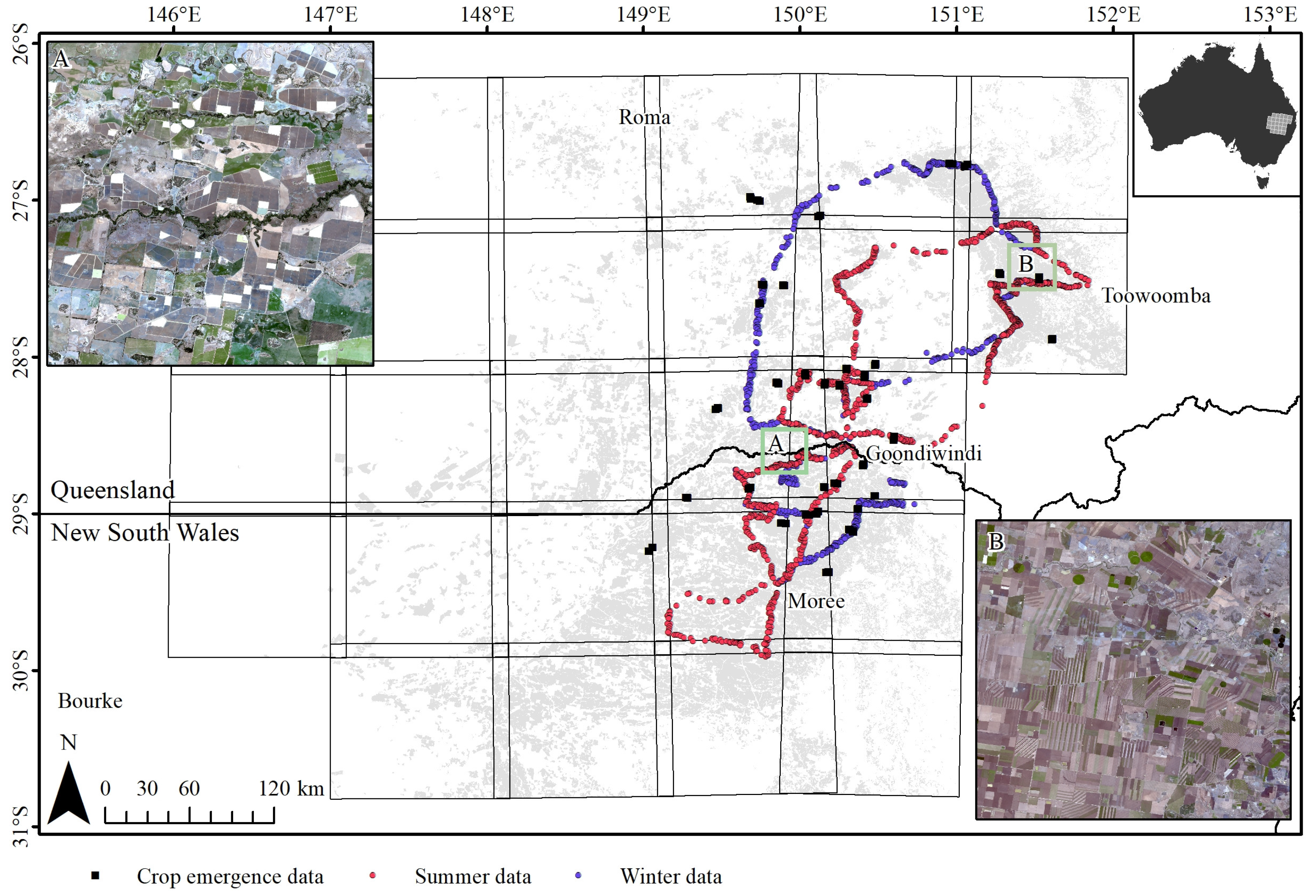
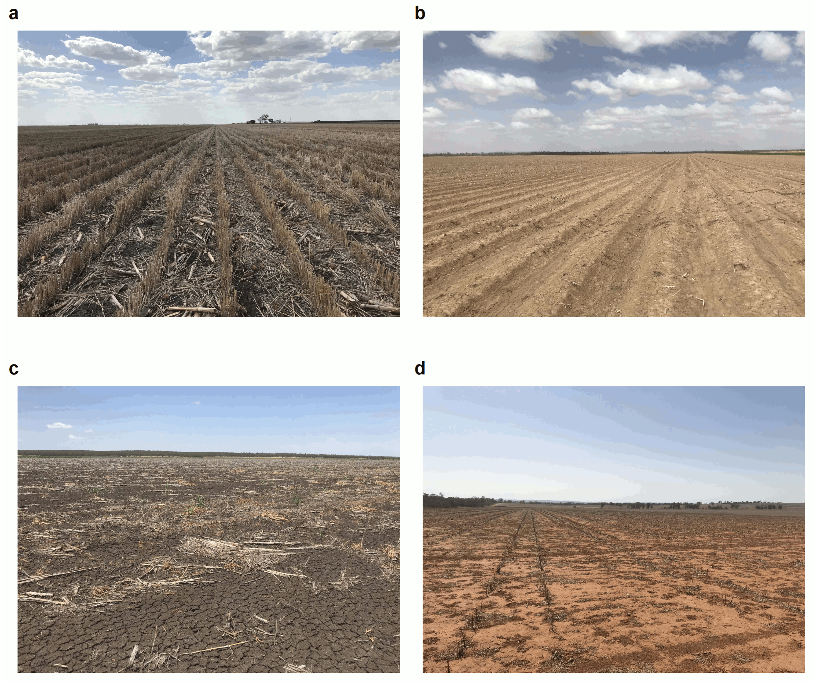
This study focused on an area of circa 250,000 km in the northern grains region of Australia (northern New South Wales and southeastern Queensland; Figure 1). Soil types vary from grey, brown, or black vertosols to red or brown sodosols and red or brown chromosols [31] resulting in strong variations of soil colour (Figure 2). Availability of water is the main factor limiting crop productivity across the region. Most cropping is located between the 500 mm and 650 mm average annual rainfall isohyets. Annual rainfall is summer-dominant and extremely variable, especially in the north and west, with the result that cropping systems have increasingly evolved around opportunistic cropping rather than fixed rotations [32]. Planting for the summer season starts as early as September and harvests can last until late June while the winter season spans from April to December. For cereal crops grown for grain, double-cropping on a routine basis is not regularly practised due to the risk of crop failure as a result of water stress [33]. Previous studies in the area of interest evaluated the cropping intensity from 0.29 to 1.33 crops per year with an average of 0.94 [34]. Cropping intensity can be as low as 58% in the western and northern areas where rainfall is less reliable [32].
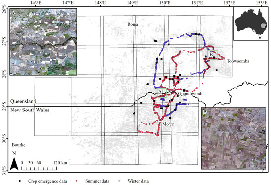
Figure 1.
Location of the area of interest and of the reference data available for training and calibration. Grey areas represent the cropping areas as mapped in ACLUM. Insets A and B correspond to natural-colour Sentinel-2 images acquired on 2017/09/07. Inset A shows an area in the Goondiwindi region, where irrigated cotton is dominant (farm dams can be seen in white); inset B displays a dryland system in the Toowoomba region, where strip cropping is commonplace.
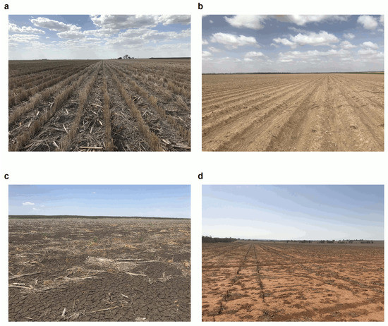
Figure 2.
Types of fallow observed in the area of interest: (a) stubble following a cereal crop; (b) bare soil prepared for a cotton crop; (c) sparse weed cover with sorghum stubble; (d) stubble of skip-row dryland cotton.
Fallows can be characterised according to their duration (short or long), weeds control (chemical or mechanical) and stubble management (stubble retention rate, stubble grazing, wind-rowing, or burning). During long fallows, fields are taken out of production for 12 to 18 months during which weeds are managed so that soil water accumulates. Short fallows last for a shorter period, typically a growing season. During summer fallows (a 5–7-month period between the harvest of last season’s winter crop and the sowing of this season’s wheat crop), rainfall events in excess of 20–30 mm can infiltrate below the evaporative zone and be stored for subsequent crop growth [35]. Fallows of 12–18 months are commonly used to transition from summer to winter crops [32]. Cultivated fallows involve repeated use of tillage implements whereas chemical fallows involve repeated use of non-residual herbicides to control weeds. The advantage of chemical fallows in years of low rainfall and yield potential was shown to result from greater water conservation (53 mm year on average [36]). Efficiency of water capture and use by crops has further been improved by conservation tillage as well as no-till and crop residue retention which has been widely adopted across Australia [37]. The range of stubble management options, e.g., windrowing, can lead to a wide diversity of spectral signatures. All these factors contribute to generating a wide diversity of fallow types across the study area (Figure 2).
2.2. Remotely-Sensed Data and Cropland Map
We sourced 7039 Sentinel-2 images from the Sentinel Australasia Regional Access (SARA; https://copernicus.nci.org.au) covering 25 tiles from 1 January 2017 to 16 November 2019. They were pre-processed following the approach described in Flood et al. [38], which retrieves surface reflectance [39], eliminates bidirectional reflectance effects [40], and masks out water, clouds and cloud shadows [41].
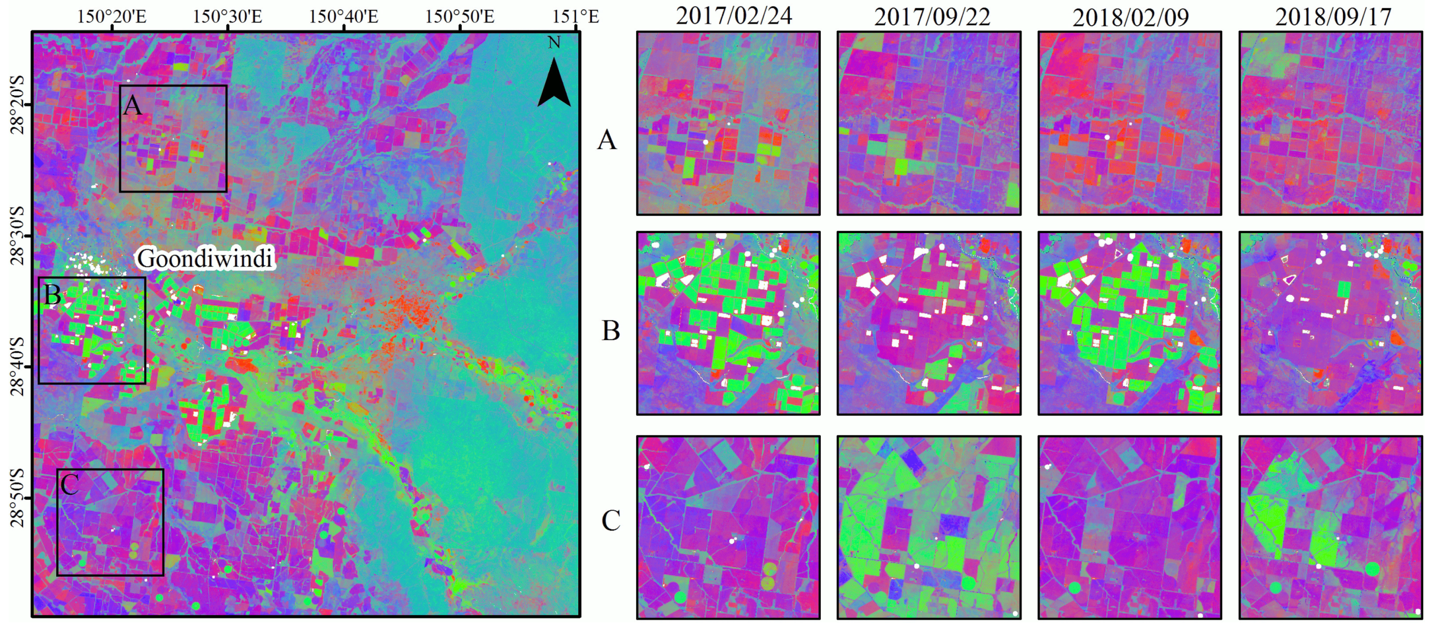
We capitalised on an existing algorithm developed under Australian conditions to convert surface reflectance into cover fractions [42,43,44]. This algorithm uses linear unmixing to quantify the photosynthetic (PV), the non-photosynthetic (NPV) vegetation, and the remaining fraction of bare soil (BS) in each pixel. The unmixing model was initially calibrated with Landsat data based on 1500 in-situ observations covering a wide variety of vegetation, soil and climate types across Australia [42,43]. All in-situ observations were recorded between July 2002 and January 2013 and were concentrated during the southern-hemisphere autumn, winter and spring. The model uses six spectral bands (blue, green, red, near infrared, and two shortwave infrared bands). It sets a hard positivity constraint and a soft sum to 1 constraint, i.e., the model needs to optimise solving for the end member abundances, not that they should sum to one (although they generally do). This initial unmixing model retrieved cover fractions with a Root Mean Squared Error (RMSE) of 11%. Following a cross-sensor calibration procedure, it was recently adapted to Sentinel-2 images to provide a 10-m product, which necessitated resampling all 20-m bands to 10 m using bicubic convolution [44]. With these reflectance adjustments, the coefficients of determination (R) between Landsat and Sentinel-2 bands were and the RMSEs were . Consequently, cover fractions retrieved from Landsat and Sentinel-2 thus strongly agree (R; RMSEs ). The output of the retrieval process is a 10-m four-band image: the first three bands corresponding to the cover fractions (PV-NPV-BS; see Figure 3) and the last band to the model fitting error, which was discarded in further analyses.
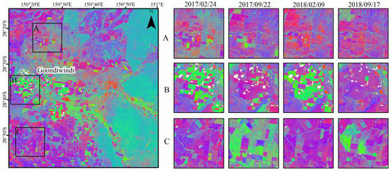
Figure 3.
Fractional cover products in the vicinity of Goondiwindi (Queensland) for several dates. Images present the fractional cover in RGB with R = bare soil, G = photosynthetic vegetation, B=non-photosynthetic vegetation. Insets A, B, and C are 15 km × 15 km.
We sourced detailed information about the cropland extent in Queensland and New South Wales from the Australian Land Use and Management (ALUM) classification (www.agriculture.gov.au/abares/aclump/land-use/data-download). Land use information at catchment scale has been produced for all states in Australia with dates and scales varying depending on when the data was collected and the intensity of land use. ALUM provides a three-tiered hierarchical structure, with primary, secondary and tertiary classes structured by their potential degree of modification and their impact on an initial land cover [45]. The land use features were manually digitised based on visual interpretation of multi-temporal satellite imagery, digital orthophotos, scanned aerial photography as well as ancillary data sets containing land use information and field observations. The reliability scale is 1:10,000 for New South Wales and 1:50,000 for Queensland. At a scale of 1:50,000, the area of the smallest mapped object is two hectares and the minimum width for linear objects is 50 m. The “cropping” class defined the extent of the cropland in our area of interest. It includes categories such as cereals, hay and sillage, oilseeds, cotton, or pulses. Cropland might be over-estimate because areas of pasture which appeared to be harvested for fodder or grazed often were mapped as “cropping”. Overall, ALUM provides an accurate, complete and consistent description of land uses and of the cropland extent across our area of interest.
2.3. Reference Data
We collected reference data during two roadside surveys in September 2017 (winter season) and January 2018 (summer season). Roadside data collection has been shown to be a viable sampling approach for training data collection providing environmental and management gradients are surveyed [46]. For fallow mapping in the northern grains region of Australia, these gradients involve changes in soil colour, soil moisture, stubble retention and tillage. Previous research concluded that changes soil colour or soil moisture did not significantly influence model performance [43]. Sample selection biases are unlikely because fields were observed from a range of roads, from primary roads to dirt tracks. Therefore, sample selection biases due the survey method were unlikely. Field boundaries associated with each point-based label were subsequently drawn using Google Earth and in-season Sentinel-2 imagery. A total of 2009 ground-truth polygons were at hand of which 1133 were collected during summer and 876 were collected in the winter (Figure 1). The average field size was 50 ha (5000 pixels).
A second data set consisting of 44 geolocated data points was collected by private agronomists who visited these fields weekly and recorded emergence when half the plants along a 1-m transect in the sowing row reached emergence.
3. Methods
Our objective was to develop a method to map fallows in near real-time across the northern grains region of Australia. To increase the temporal coverage of field data and reduce fieldwork, we assumed, based on domain knowledge, that fallow labels could be extended across the first half of the growing season. Indeed, the cover fractions of fallows are likely to remain stable over time because, in the northern grains zone of Australia, good management practices involve spraying weeds soon after they emerge. As a result, fallow labels collected during flowering, i.e., when the fallow extent is minimal, can be extended to the first half of the season, thereby extending the temporal coverage of positive data at no cost. By contrast, crop labels cannot be extended because their emergence date is unknown. At best, they can be considered unlabelled, which prevents the use of conventional classifiers and justifies the one-class approach.
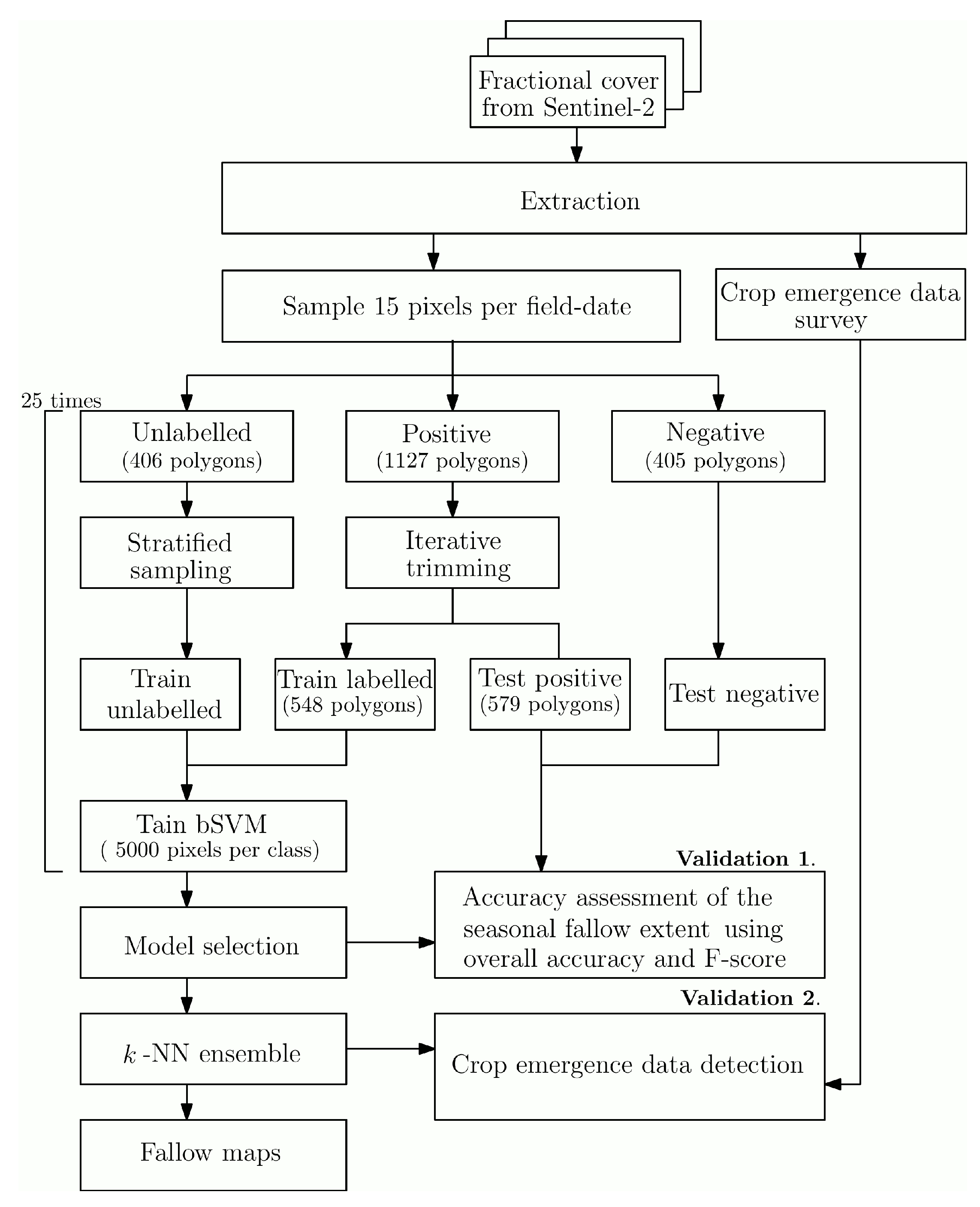
Based on these principles, our classification method has four main steps (Figure 4): (1) extracting fractional cover values and outlier removal; (2) sampling labelled and unlabelled data to generate training and validation sets; (3) training and selecting optimal classifiers; and (4) validating the seasonal fallow extent maps and dynamic fallow detection.
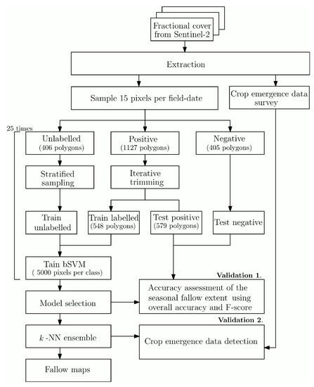
Figure 4.
Flowchart of the proposed classification approach.
3.1. Data Pre-Processing And Resampling
We extracted positive, negative, and unlabelled data from the field observations. The extraction period spanned from 6 April to 2 September for the winter season and from 10 October to 20 January for summer season. To provide reliable estimates of the space-time generalisation accuracy, the surveyed fields were split into two independent sets of polygons (50:50): one set was used for training classifiers and the other for validation. We randomly selected 15 pixels per field-date for both the positive and unlabelled data to reduce redundancy in the data.
Outliers can significantly impact the performance of one-class classifiers [24,25]. As positive data contained outliers due to imperfect cloud and shadow masking, we removed them using nonparametric iterative trimming [47]. Iterative trimming identifies outliers from the data by estimating the probability density function of the data distribution, then removes all data points with a probability density estimate smaller than . Thus, controls how much data are removed in each iteration. This procedure was repeated until no new outliers were identified. Kernel density estimates were obtained using binned kernel approximations [48], which are suitable when a large number of observations are at hand. We tested five values of and selected the optimal one by cross-validation (Table 1).

Table 1.
Parameters of the model optimised by cross-validation.
Given the sheer number of positive and unlabelled pixels, we generated 25 smaller, more manageable training sets of 10,000 pixels (5000 pixels per class) using bootstrapping (iterative sampling with replacement). Positive data were randomly drawn. Unlabelled data were selected following a stratified sampling that maximised the spatial coverage of the feature space. A total of 3228 strata were defined by tessellation of the feature space in regular triangles. Each side of the triangular strata had a length of two per cent fractional cover. We then randomly selected 5000 samples with a maximum of two samples per stratum. Good balance between the positive and unlabelled classes has been shown to improve the performance of one-class classifiers [25].
3.2. Classification Method
One-class classifiers are well-established in remote sensing. They can be grouped in two groups: P-classifiers and PU-classifiers. P-classifiers use only positive data for training, PU-classifiers use both positive and unlabelled data. P-classifiers can lead to unreliable results when the training sample is less representative or when the positive data is insignificantly different from the other class. Therefore, we implemented biased Support Vector Machines (bSVM [49]), a PU-classifier adapted from binary Support Vector Machine [50]. Empirical evidence showed that bSVM performs better than other one-class classification methods [51].
The bSVM classfier transforms the original training set into a high dimension space and constructs a hyperplane that maximises the margin between two or more classes. The margin is the distance from the hyperplane to the closest element on either side. It also includes a regularisation parameter C, which controls the trade-off between maximising the margin and minimising the training error. The core concept of bSVM is to penalise classification errors differently depending on whether the misclassified data were labelled or not [49]. As a significant amount of the unlabelled set will contain positive data, it is relevant to penalise misclassifications of positive data more strongly than of unlabelled data. Thus, misclassification cost terms are defined for each class so that and are the regularisation for positive and unlabelled data, respectively. Our implementation used rather than , which is a multiplier used to define the penalty of positive class based on the regularisation term of the unlabelled class, i.e., .
We selected Gaussian radial basis functions as kernel for the bSVM models in order to create non-linear classifiers. The inverse kernel width () as well as and were optimised using grid search (Table 1).
3.3. Model Selection
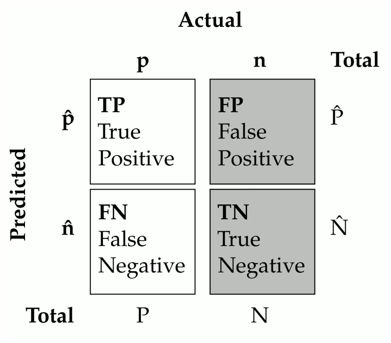
Models are generally selected based on accuracy measures which are derived from the error matrix (Figure 5). In the context of binary or multi-class classification, an array of accuracy metrics is available [52]. The overall accuracy provides the proportion of pixels that were correctly classified:
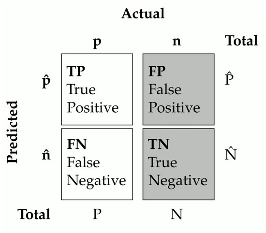
Figure 5.
Illustrative error matrix. Shaded areas represent data that are not available for one-class classifier selection. P, N, , represent the number of positive and negative samples, and the number of samples classified as positive and negative.
The true positive rate (TPR), also known as the producer’s accuracy, is the proportion of correct conditions of positive cases (true positive) over the number of actual negative cases in the data:
The precision, or the user’s accuracy, indicates the probability of correctly detecting a positive case:
The F-score is the harmonic mean of precision and true positive rate [53]:
Precision is not available for one-class problems because only positive samples are known. This poses serious challenges because, if only the true positive rate can be computed, a classifier would naturally tend to classify all data as positive. Thus, specific accuracy metrics have been proposed to capture the specifics of one-class classification. A reliable one-class classifier minimises the number of unlabelled data classified as positive and maximises the amount of positive data that are correctly classified [54]. An oft-used metric is the probability of positive prediction (PPP) that estimates the ratio of pixels classified as positive:
where the total number of observations is given by N+P. A second common metric is PU-performance (puF) which is related to the F-score and combines TPR and PPP [55]:
It follows that the higher the puF, the more accurate the one-class classifier.
Evidence showed that modifying the decision threshold is an inexpensive optimisation that can lead to significant improvement of performance measures [30,51,56]. The bSVM model produces continuous predictions and a threshold is needed to separate the positive and negative classes. By default, this threshold is 0. Piiroinen et al. [54] proposed an approach (herein the min.dist approach) to select the optimal threshold based on the Receiving Operating Characteristics (ROC) curve adapted for one-class problems and on the concept of Pareto dominance. The ROC curve was adapted for one-class classification problems so that TPR is the y-axis and PPP the x-axis. The rationale of the min.dist approach is that the most accurate classifiers have a high TPR and low PPP, i.e., they should be located as close as possible to the upper left corner of the ROC curve plot (TPR = 1 and PPP = 0). The classifier with the optimal threshold is thus the closest to the top-left corner in the TPR-PPP space.
We compared the puF and min.dist models. We tested 50 different thresholds for every combination of parameters to generate the min.dist candidate models. In total, we generated 5 million bSVM models (50 thresholds × 5 values × 10 values × 8 values × 10 values × 25 repetitions). We then assessed the accuracy of the models selected by the two approaches for seven periods of 20 days ranging from 4 April to 2 September and 10 October to 20 January for the winter and summer seasons, respectively. Within each 20-day period, we only considered the predictions of the latest cloud-free observations for each pixel. We selected the best approach based on their overall accuracy and F-score. We assessed the statistical significance of their differences by means of t-tests.
3.4. Assessing the Model Performance and Building an Ensemble
3.4.1. Validating Seasonal Fallow Predictions
As for model calibration, ground truth data distributed along the growing season were lacking. Therefore, we validated the outputs of the bSVM models in two steps: first, we validated maps of the seasonal fallow extent and assessed how soon it could be reliably mapped; and second, we evaluated the accuracy of the dynamic fallow detection during the season using crop emergence data.
The accuracy of seasonal fallow extent was evaluated using an independent set of ground truth data for both the summer and winter seasons. Positive data were derived from bootstrapped subsets of the fallow polygons (579 polygons on average) and negative data were randomly selected from crop observations (405 polygons; Figure 4). Ground truth labels were then compared against those provided by the classifiers for images within a 20-day window around the field survey date so as to fill in gaps due to missing values. To assess performance at both the overall and class levels, we computed the overall accuracy (OA; Equation (1)), the true positive rate (TPR; Equation (2)), the precision (Equation (3)), and the F-score (Equation (4)) across the 25 bootstrapped samples. We compared the accuracy between every mapping period and survey date period using t-tests. Statistical significance was declared if differences in accuracy were > 5%. Note that a decline in accuracy does not automatically imply poor model performance but rather indicates that some late sown crops may not have been sufficiently developed to be remotely distinguished from fallows.
3.4.2. Building an Ensemble
Ensuring a low computational cost is essential for near real-time monitoring applications that need to run at scale. Thus, for inference, we combined the selected models (trained from the 25 training sets) into an ensemble. To that purpose, we applied the 25 bSVM models to every combination of cover fraction regularly spaced by 1% cover, which is the resolution of the retrieval algorithm. The class of each grid point was then determined by majority voting. The ensemble was a k-nearest neighbour (k-NN) algorithm with k set to 1. We benchmarked the CPU time of a single bSVM model against that of the k-NN ensemble. We reported the average CPU time of each approach to process 100 randomly-selected and cloud-free Sentinel-2 images and assessed their difference with a Wilcoxon signed rank test.
Our implementation ran in R version 3.5.0 and relied on the raster, caret, kernlab and oneClass packages. All computations took place on a Dell PowerEdge M630 system where each classification was allocated ten Dual 10 core Intel Xeon E5-2660 V3 processors running at 2.6 GHz with 25 MB cache and 10 GB of RAM.
3.4.3. Validating Near Real-Time Performances
We assessed the accuracy of the dynamic fallow detection by comparing reported and detected crop emergence dates at 71 locations across the study area for the 2017 winter season. For each location, the detected emergence date was defined as the first occurrence of the longest series of non-fallow detection. The most accurate model was selected based on the results of the first validation. The reported emergence date was corrected to account for the delay between emergence and the first actual satellite overpass. We evaluated the agreement between observed and detected crop emergence dates with the and RMSE.
3.5. Mapping the Seasonal Fallow Dynamics
To map the fallow dynamics for six sequential seasons from 2017 to 2019, we classified all images between January and February, and September and October. Then, we summarised all classifications in the period of interest using a mode algorithm to reduce the impact of missing values. We also calculated the fallowed and cropped areas in the period of interest and drew the dynamical flow of cropping from summer 2017 to winter 2019.
4. Results
4.1. Model Selection: puF vs. min.dist
For each of the 25 bootstrapped samples, we trained 200,000 models and selected the best ones following the puF and min.dist criteria. The best models had the following parameters: = 10, = 5.1, = 2, = 0.01 for puF and = 10, = 9.1, = 2, = 0.01 and threshold = 0.938 for min.dist. To compare the best puF and min.dist models, we calculated the average overall accuracy and F-score based on the closest cloud-free observations to the survey dates (Table 2). Both methods achieved high overall accuracy (0.86–0.94) and F-score (0.88–0.94). Tuning the threshold of the decision boundary (min.dist) did not provide a significant increase in accuracy compared to the default decision threshold (puF). Therefore, we retained the bSVM models with the highest puF because they were less computationally demanding to train.

Table 2.
Accuracy metrics obtained from comparison of the classification results with an independent test set from winter 2017 and summer 2018. The accuracy and F-score values are means of 25 iterations with different sub-samples of the reference data.
4.2. Accuracy of Seasonal Fallow Maps and Crop Emergence Detection
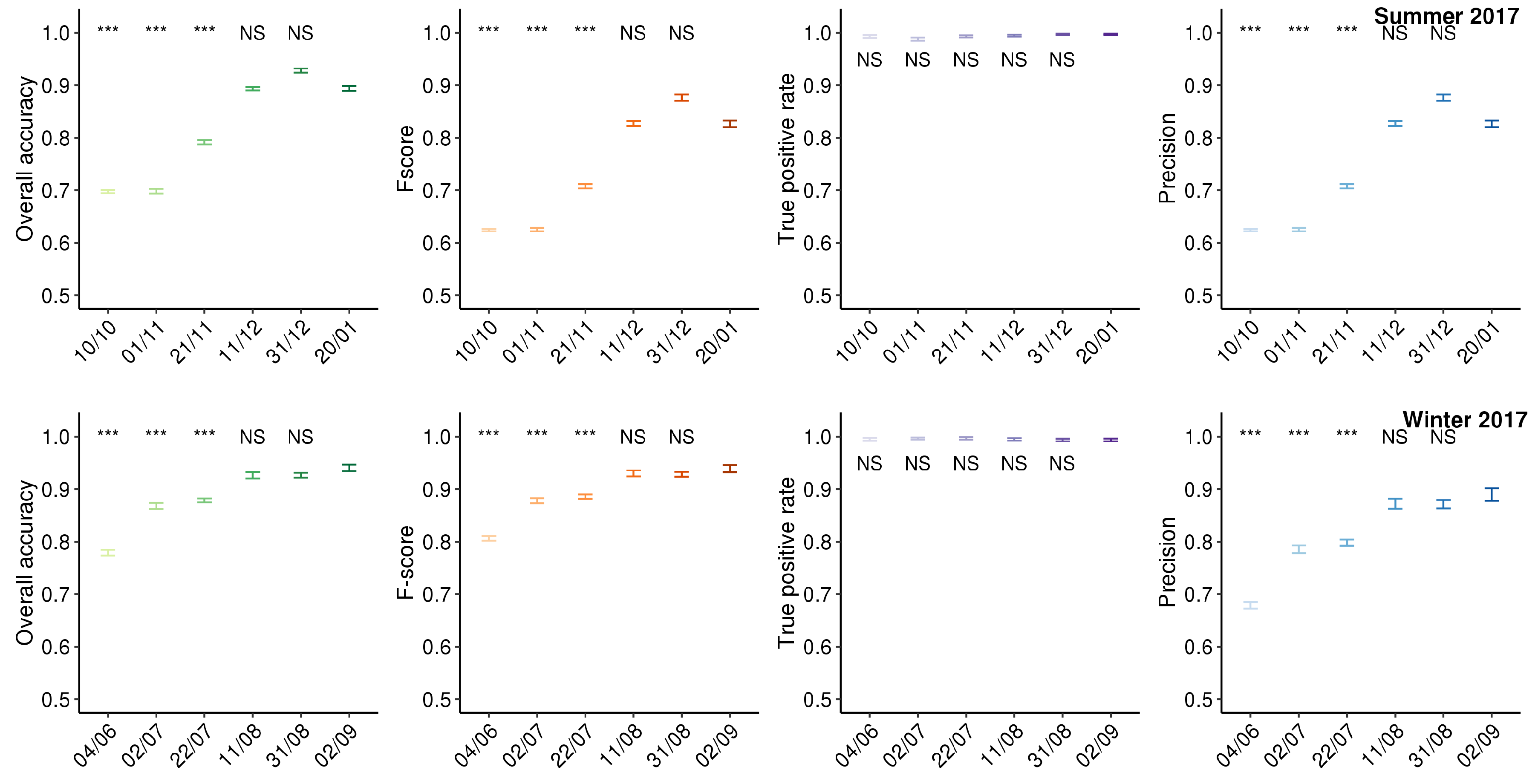
We applied the best puF models to fractional cover images for six 20-day periods preceding the survey to identify how early reliable maps of the fallow extent could be obtained. We then computed the corresponding overall accuracy, F-score, true positive rate, and precision (Figure 6). In winter 2017, the overall accuracy, the precision and the F-score reached about 92% for early August and continued to grow up to 94% in early September. It is important to stress here that the majority “errors” are not actual errors but rather they indicate limitations of extending crop labels prior to crop emergence. The true positive rate did not drop below 99%, indicating that fallows were marginally missed. Accuracy differences were not significant from mid-August on (Wilcoxon tests; p-values > 0.05). Therefore, we concluded that the winter fallow extent could be determined as early as mid-August (or 2–4 months before harvest).
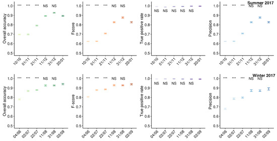
Figure 6.
Accuracy of the seasonal fallow extent predictions over time. NS indicates non-significant differences while *, ** and *** indicate significant differences at the 95%, 99% and 99.9% confidence levels.
With the exception of a slight decrease in late January, similar trends were observed in the summer of 2018. The overall accuracy, the F-score and the precision reached about 90% in late December and decreased to 85% in late January. The true positive rate maintained high accuracy (99%) throughout the season. The drop of accuracy at the end of January ought to be related to the larger sowing windows for summer crops than for winter crops. For instance, sorghum can be sown from early September to late February. Harvests of early-sown sorghum can occur while late-sown sorghum is still maturing. Differences in accuracy were significant until mid-December. Therefore, we concluded that the summer fallow extent could be mapped from mid-December onwards (or 1–4 months before harvest).
The median run time for a single bSVM for processing a cloud-free Sentinel-2 image was 2.7 h (i.e., 67.5 h are necessary for all 25 models of the ensemble to complete). In comparison, the k-NN ensemble ran in 2.5 h, which was a significant reduction in run time (p-value = 0.0450). The ensemble successfully integrated the 25 bSVM models for less than the computational cost of a single bSVM model.
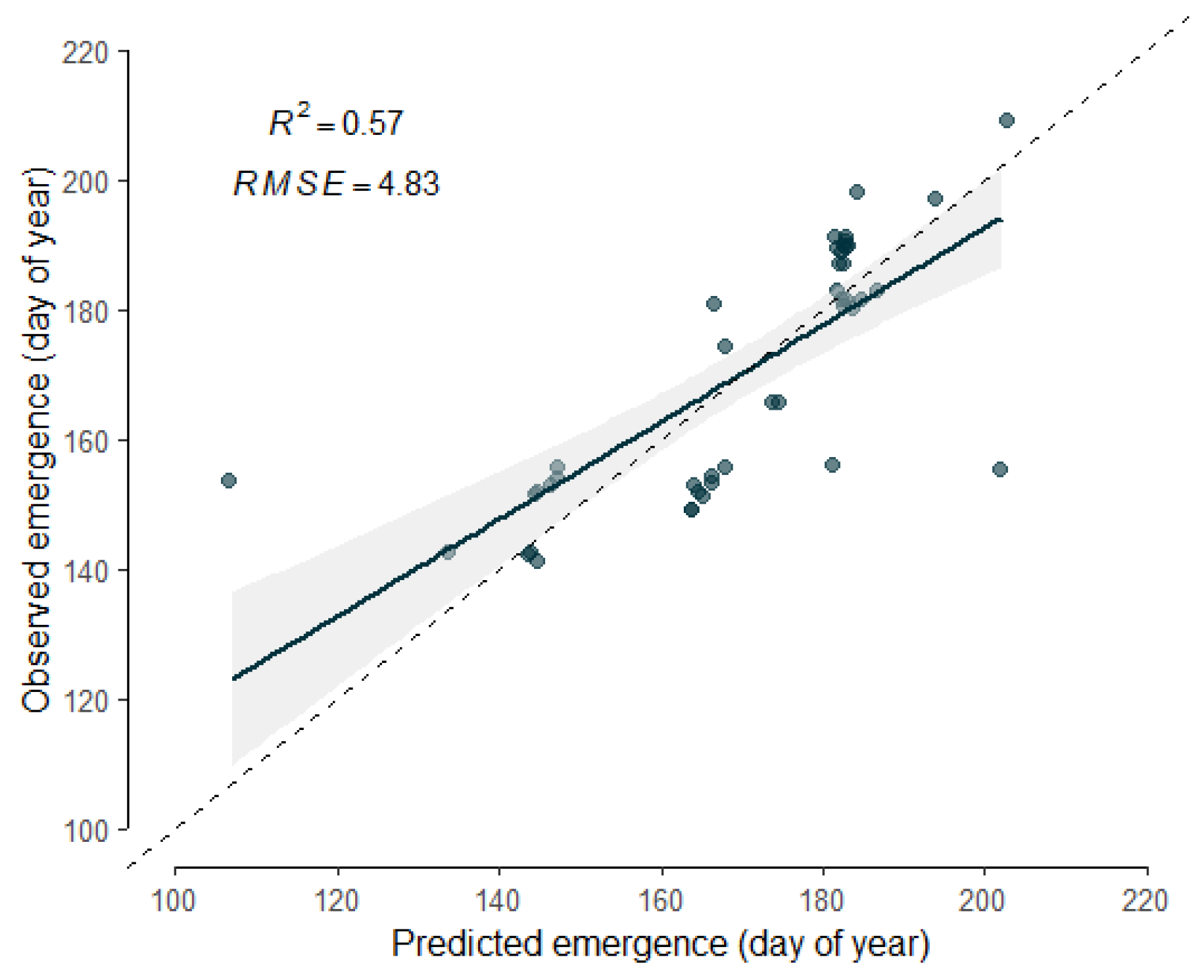
To validate the near real-time detection performance of the ensemble, we compared predicted crop emergence dates against reported ones (Figure 7). The regression had an of 0.57 and an of 4.8 days, which underlines the model’s ability to detect land-use changes in near real-time.
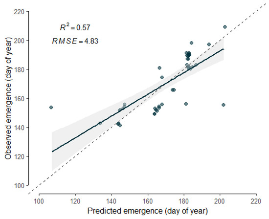
Figure 7.
Relationship between the predicted and the reported emergence dates. ( = 4.83 days; = 0.57; p-value < 0.01)
4.3. Mapping the Seasonal Fallow Extent and the Cropping Dynamics
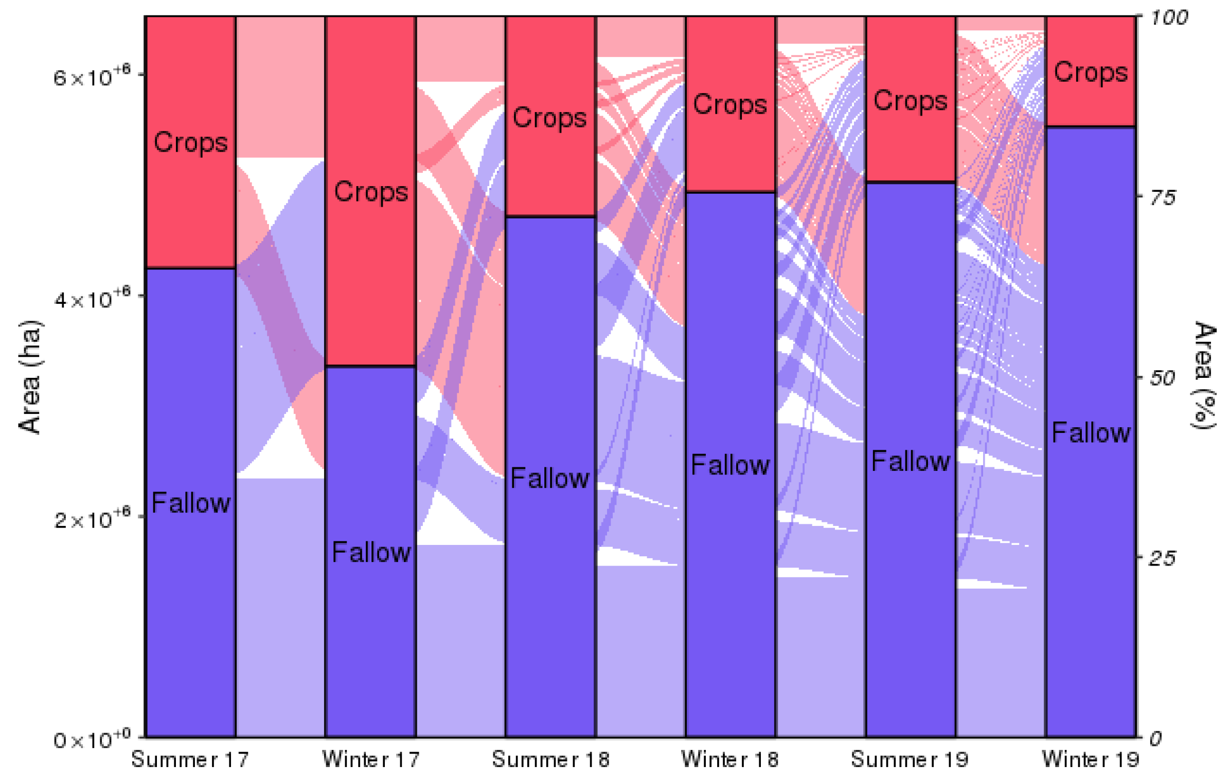
We mapped the seasonal fallow extent for six consecutive seasons from summer 20107 to winter 2019 using the ensemble. Then, we calculated the flow of pixels between the fallow and the cropping pools (Figure 8). Estimates suggested that 20% of the cropland area had a cropping intensity of 2, 30% of 1.5, 23% of 1, 11% of 0.5, and 16% of 0. Pixels with a cropping intensity of 0 were largely found in the western fringe of the cropping area where rainfall is less reliable. The seasonal fallow extent ranges between 50% in winter 2017 (3.3 million ha) and 85% in winter 2019 (5.6 million ha), which underlines the importance of fallowing in the study area. Due to dry conditions across the study area, the cropped area kept on decreasing since record high winter-crop production was achieved in 2016–2017 [57]. The large extent of winter fallows in 2018 and 2019 is consistent with official reports [57,58]. It is related to a lack of sowing opportunities or failed crop establishment because of drought conditions across south-east Queensland and northern New South Wales.

Figure 8.
Cropping dynamics in the study area from summer 2017 to winter 2019.
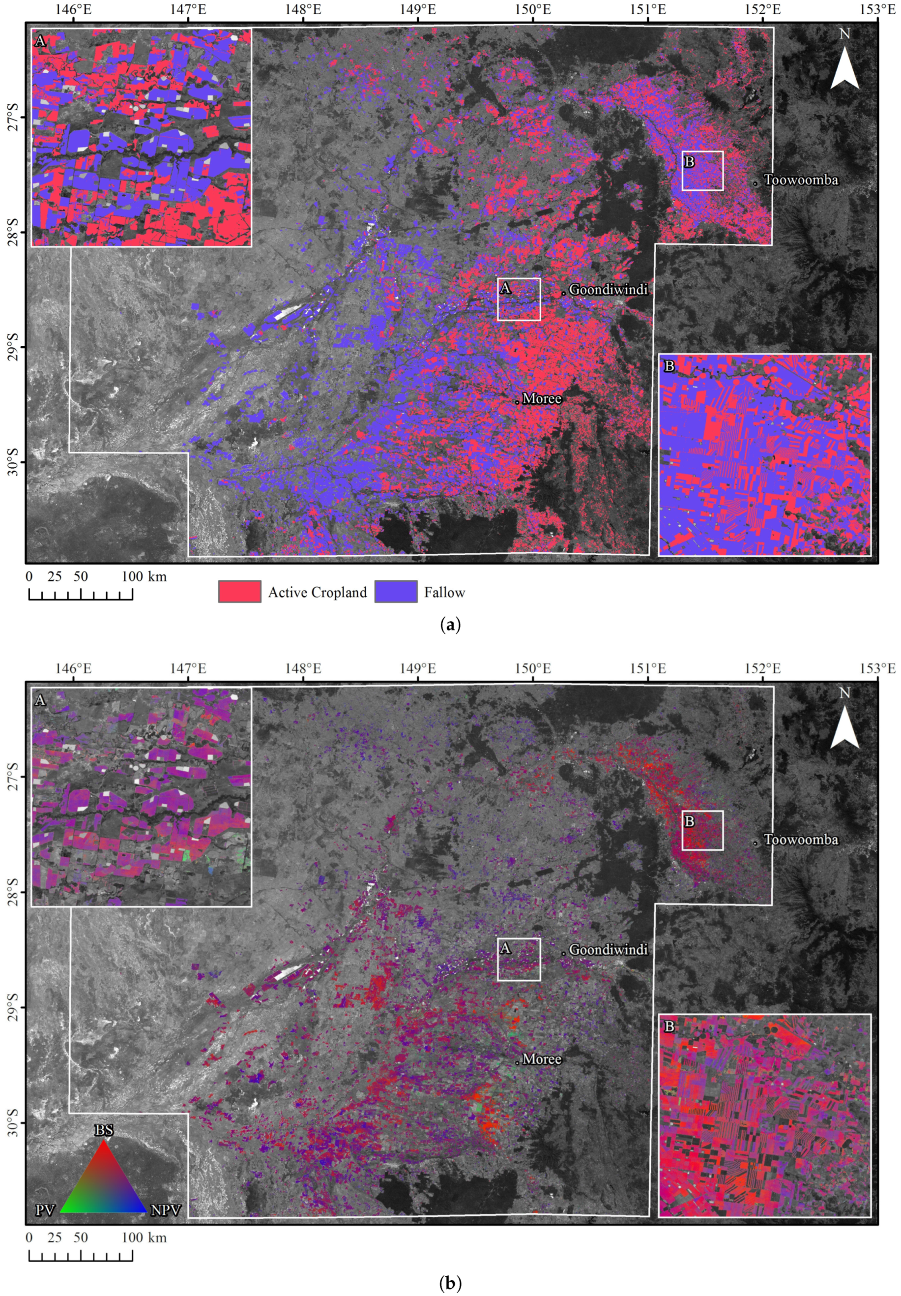
The fallow extent maps captured spatial and temporal patterns in agreement with domain knowledge (Figure 9a). For instance, most fallows were located on the western fringe of the cropping area, which is, on average, drier (500–550 mm of annual rainfall) than the eastern part of the study area (550–750 mm). Fields near dams were largely fallowed before being sown with irrigated cotton crop, which is more profitable (Figure 9b inset A). The average bare soil fraction, photosynthetic fraction and non-photosynthetic fraction were 55%, 10%, and 35%, respectively.
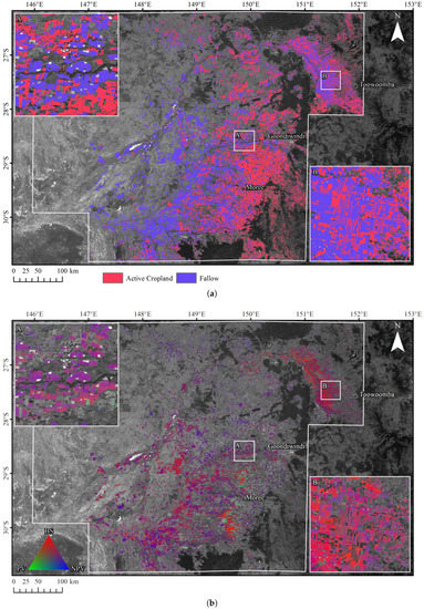
Figure 9.
Maps of (a) the winter 2017 fallow extent and (b) the corresponding cover fractions.
5. Discussion
In this paper, we introduced a new method to estimate the location and extent of fallows across the northern grains region of Australia based on one-class classifiers and fractional cover data. Our method can use single fractional cover images derived from Sentinel-2 at any point in time without re-calibration. The final classifier is an ensemble of 25 bSVM base models with low computing costs and is, therefore, well-suited for repeated, large-scale applications.
The level of accuracy of our method seems to indicate that it is fit for several purposes. First, accurate estimates of the seasonal fallow extent could be obtained by mid-August and mid-December for winter season and summer season respectively (1–4 months before harvest). They can inform early-season estimates of the area cropped, well ahead of the optimal window for crop identification. For instance, the best temporal window for single-date classification of summer crops in south-eastern Australia was February to mid-March [59]. Such timely information would be particularly valuable during drought-stricken years. Second, near real-time information about the extent and location of fallows combined with pixel-level photosynthetic vegetation cover fractions can provide insights about the weed populations that need to be controlled, and therefore are a proxy for herbicide demand. In the region of interest, herbicides represent one of the largest costs to grain growers [60]; not controlling weeds results in a direct loss of yield potential. Third, the model’s ability to detect crop emergence seems promising. Recent attempts to identify sowing dates have leveraged hyper-temporal and hyper-spatial resolutions of CubeSats (e.g., [61]) but these can hardly be scaled due to the cost of such data. While more work is needed to deal with one-off false negatives (false detection of crops), deriving crop emergence from time series of fallow maps is an interesting alternative to most time series approaches which cannot provide timely estimates of crop emergence. Overall, our approach seems fit to serve a range of applications in the study area. We expect that it would perform equally well in other regions of the Australian wheat belt as well as in other cropping systems, where rainfall is the main factor limiting crop production.
One of the benefits of our method is that it reduces the data collection effort to a single roadside survey during the flowering period, which is similar to the surveys used for cropland or crop type mapping [46,62]. We then extended the labels observed around flowering back in time (beyond crop emergence) based on assumptions supported by the knowledge of local fallow management practices. The net effect was a more comprehensive class description, accompanied by a dramatic increase of the number of pixels available for training. We reduced the sample size by randomly sampling 5000 pixels per class. Each bSVM model was trained with data from around 550 fields labelled as fallows and 400 unlabelled crop fields. If the latter are not available, they can be obtained by sampling randomly within the cropland area. The training set size might have been further reduced with minimal impact on the classification accuracy by using more advanced data selection methods are likely to perform [21,22,23]. The ability to lower data collection requirements is advantageous for large-scale applications.
We reduced sensor dependence by choosing cover fractions instead of spectral data. This entails that our model can be ported to other sensors or can integrate data from multiple sensors to coverage in cloud-prone areas. In fact, the unmixing model used was first developed from Landsat. As a result, our approach can make use of the whole archive of Landsat fractional cover products to highlight changes in the fallow patterns or reconstruct spatially the trend towards early sowing [63]. Both in hindcast and nowcast, our model enables several interesting cross-platform national-scale applications. It could readily be deployed on the Australian Geoscience Data Cube [64], which provides timely processing of big earth observation data through its integration within the high-performance computing environment provided by the Australian National Computational Infrastructure.
The fundamental goal of this works was to develop a method for operational fallow monitoring as well a data for future research on cropping dynamics in Australia. This study advanced the capabilities for near real-time monitoring of agriculture in Australia with little data requirements. The general lack of field data over space and time, which makes training and validation difficult, also speaks to the unique value brought in by one-class classification methods. This study also suggests several options for further improvement. Foremost among these is to reduce the uncertainty of the unmixing method (which retrieves cover fractions with an average accuracy of 11.6%) with multi-output machine learning regression models (see [65] for a review). Improvements will propagate and directly boost the accuracy of fallow detection when crop cover is low. Second, accuracy could further be improved by integrating classification outputs (and possibly domain knowledge) across time so as to reduce the occurrence of one-off detections. Third, fallow mapping will benefit from improved cropland masking. It is interesting to note that our method could be used to refine cropland maps. Applied over multiple years, it could identify areas consistently not cropped and areas with permanent vegetation cover and thus progressively improve the cropland map. Fourth, cover fractions could be used to establish a biophysical typology of fallows based for instance on crop residues. This would pave the way to studying issues such as crop residues and their impacts on soil erosion and soil organic carbon [66] or mapping the shift to agricultural systems involving no-tillage across Australia [67]. Finally, future work is needed to evaluate if harvest dates could be detected.
6. Conclusions
We developed a new method to monitor the fallow dynamics in near real-time. Our method combines one-class classifiers (biased support vector machines) with fractional cover images derived from Sentinel-2. One-class classifiers allowed us, based on domain knowledge, to extend the temporal coverage of in-situ observations collected around flowering in order to generate large training data sets, thereby reducing the data collection requirements. Fractional cover images intuitively describe fallows in biophysical terms and increase sensor independence. In the northern grains zone of Australia, the seasonal fallow extent was identified with an average accuracy >92% in both summer and winter. We also showed that reliable maps of the seasonal fallow extent could be obtained as early as mid-August for the winter season (2–4 months before harvest) and mid-December for the summer season (1–4 months before harvest). The method’s ability to identify fallows in near real-time was verified using crop emergence data (R = 0.57). The final classifier was a simple ensemble of 25 one-class classifiers, which significantly reduced computational costs so that inference across large areas is fast. Our method can readily be transferred to other sensors and implemented on the Australian Geoscience Data Cube. This paper provides a clear pathway towards operational monitoring of the fallow and cropland dynamics across Australia.
Author Contributions
L.Z.: Methodology, Software, Formal analysis, Visualisation, Writing—original draft. F.W.: Conceptualisation, Visualisation, Writing—original draft, Writing—review & editing. P.S.: Resources, Writing—original draft, Writing—review & editing. B.M.: Software, Writing—original draft, Writing—review & editing. Z.H.: Resources, Supervision, Writing—original draft, Writing—review & editing. All authors have read and agreed to the published version of the manuscript.
Funding
The authors acknowledged the support of the Digiscape Future Science Platform, funded by the CSIRO.
Conflicts of Interest
The authors declare no conflict of interest.
References
- French, R. The effect of fallowing on the yield of wheat. I. The effect on soil water storage and nitrate supply. Aust. J. Agric. Res. 1978, 29, 653–668. [Google Scholar] [CrossRef]
- French, R. The effect of fallowing on the yield of wheat. II. The effect on grain yield. Aust. J. Agric. Res. 1978, 29, 669–684. [Google Scholar] [CrossRef]
- Siebert, S.; Portmann, F.T.; Döll, P. Global patterns of cropland use intensity. Remote Sens. 2010, 2, 1625–1643. [Google Scholar] [CrossRef]
- Wu, Z.; Thenkabail, P.S.; Mueller, R.; Zakzeski, A.; Melton, F.; Johnson, L.; Rosevelt, C.; Dwyer, J.; Jones, J.; Verdin, J.P. Seasonal cultivated and fallow cropland mapping using MODIS-based automated cropland classification algorithm. J. Appl. Remote Sens. 2014, 8, 083685. [Google Scholar] [CrossRef]
- Melton, F.; Rosevelt, C.; Guzman, A.; Johnson, L.; Zaragoza, I.; Verdin, J.; Thenkabail, P.; Wallace, C.; Mueller, R.; Willis, P.; et al. Fallowed Area Mapping for Drought Impact Reporting: 2015 Assessment of Conditions in the California Central Valley; NASA AMES Research Center: Mountain View, CA, USA, 2015.
- Gumma, M.K.; Thenkabail, P.S.; Teluguntla, P.; Rao, M.N.; Mohammed, I.A.; Whitbread, A.M. Mapping rice-fallow cropland areas for short-season grain legumes intensification in South Asia using MODIS 250 m time-series data. Int. J. Digit. Earth 2016, 9, 981–1003. [Google Scholar] [CrossRef]
- Tong, X.; Brandt, M.; Hiernaux, P.; Herrmann, S.; Rasmussen, L.V.; Rasmussen, K.; Tian, F.; Tagesson, T.; Zhang, W.; Fensholt, R. The forgotten land use class: Mapping of fallow fields across the Sahel using Sentinel-2. Remote Sens. Environ. 2020, 239, 111598. [Google Scholar] [CrossRef]
- Bégué, A.; Arvor, D.; Bellon, B.; Betbeder, J.; De Abelleyra, D.; PD Ferraz, R.; Lebourgeois, V.; Lelong, C.; Simões, M.; R Verón, S. Remote sensing and cropping practices: A review. Remote Sens. 2018, 10, 99. [Google Scholar] [CrossRef]
- Fritz, S.; See, L.; Bayas, J.C.L.; Waldner, F.; Jacques, D.; Becker-Reshef, I.; Whitcraft, A.; Baruth, B.; Bonifacio, R.; Crutchfield, J.; et al. A comparison of global agricultural monitoring systems and current gaps. Agric. Syst. 2019, 168, 258–272. [Google Scholar] [CrossRef]
- Wardlow, B.D.; Egbert, S.L.; Kastens, J.H. Analysis of time-series MODIS 250 m vegetation index data for crop classification in the US Central Great Plains. Remote Sens. Environ. 2007, 108, 290–310. [Google Scholar] [CrossRef]
- Boryan, C.; Yang, Z.; Mueller, R.; Craig, M. Monitoring US agriculture: The US department of agriculture, national agricultural statistics service, cropland data layer program. Geocarto Int. 2011, 26, 341–358. [Google Scholar] [CrossRef]
- Löw, F.; Biradar, C.; Dubovyk, O.; Fliemann, E.; Akramkhanov, A.; Narvaez Vallejo, A.; Waldner, F. Regional-scale monitoring of cropland intensity and productivity with multi-source satellite image time series. GISci. Remote Sens. 2018, 55, 539–567. [Google Scholar] [CrossRef]
- Estel, S.; Kuemmerle, T.; Alcántara, C.; Levers, C.; Prishchepov, A.; Hostert, P. Mapping farmland abandonment and recultivation across Europe using MODIS NDVI time series. Remote Sens. Environ. 2015, 163, 312–325. [Google Scholar] [CrossRef]
- Teluguntla, P.; Thenkabail, P.S.; Xiong, J.; Gumma, M.K.; Congalton, R.G.; Oliphant, A.; Poehnelt, J.; Yadav, K.; Rao, M.; Massey, R. Spectral matching techniques (SMTs) and automated cropland classification algorithms (ACCAs) for mapping croplands of Australia using MODIS 250-m time-series (2000–2015) data. Int. J. Digit. Earth 2017, 10, 944–977. [Google Scholar] [CrossRef]
- Gumma, M.K.; Thenkabail, P.S.; Deevi, K.C.; Mohammed, I.A.; Teluguntla, P.; Oliphant, A.; Xiong, J.; Aye, T.; Whitbread, A.M. Mapping cropland fallow areas in myanmar to scale up sustainable intensification of pulse crops in the farming system. GISci. Remote Sens. 2018, 55, 926–949. [Google Scholar] [CrossRef]
- Wallace, C.S.; Thenkabail, P.; Rodriguez, J.R.; Brown, M.K. Fallow-land Algorithm based on Neighborhood and Temporal Anomalies (FANTA) to map planted versus fallowed croplands using MODIS data to assist in drought studies leading to water and food security assessments. GISci. Remote Sens. 2017, 54, 258–282. [Google Scholar] [CrossRef]
- Tong, X.; Brandt, M.; Hiernaux, P.; Herrmann, S.M.; Tian, F.; Prishchepov, A.V.; Fensholt, R. Revisiting the coupling between NDVI trends and cropland changes in the Sahel drylands: A case study in western Niger. Remote Sens. Environ. 2017, 191, 286–296. [Google Scholar] [CrossRef]
- Shao, Y.; Lunetta, R.S. Comparison of support vector machine, neural network, and CART algorithms for the land-cover classification using limited training data points. ISPRS J. Photogramm. Remote Sens. 2012, 70, 78–87. [Google Scholar] [CrossRef]
- Zhu, Z.; Gallant, A.L.; Woodcock, C.E.; Pengra, B.; Olofsson, P.; Loveland, T.R.; Jin, S.; Dahal, D.; Yang, L.; Auch, R.F. Optimizing selection of training and auxiliary data for operational land cover classification for the LCMAP initiative. ISPRS J. Photogramm. Remote Sens. 2016, 122, 206–221. [Google Scholar] [CrossRef]
- Heydari, S.S.; Mountrakis, G. Effect of classifier selection, reference sample size, reference class distribution and scene heterogeneity in per-pixel classification accuracy using 26 Landsat sites. Remote Sens. Environ. 2018, 204, 648–658. [Google Scholar] [CrossRef]
- Foody, G.M.; Mathur, A. Toward intelligent training of supervised image classifications: Directing training data acquisition for SVM classification. Remote Sens. Environ. 2004, 93, 107–117. [Google Scholar] [CrossRef]
- Foody, G.M.; Mathur, A.; Sanchez-Hernandez, C.; Boyd, D.S. Training set size requirements for the classification of a specific class. Remote Sens. Environ. 2006, 104, 1–14. [Google Scholar] [CrossRef]
- Zheng, B.; Myint, S.W.; Thenkabail, P.S.; Aggarwal, R.M. A support vector machine to identify irrigated crop types using time-series Landsat NDVI data. Int. J. Appl. Earth Obs. Geoinf. 2015, 34, 103–112. [Google Scholar] [CrossRef]
- Song, X.; Fan, G.; Rao, M. Svm-based data editing for enhanced one-class classification of remotely sensed imagery. IEEE Geosci. Remote Sens. Lett. 2008, 5, 189–193. [Google Scholar] [CrossRef]
- Chen, X.; Yin, D.; Chen, J.; Cao, X. Effect of training strategy for positive and unlabelled learning classification: Test on Landsat imagery. Remote Sens. Lett. 2016, 7, 1063–1072. [Google Scholar] [CrossRef]
- Waldner, F.; Chen, Y.; Lawes, R.; Hochman, Z. Needle in a haystack: Mapping rare and infrequent crops using satellite imagery and data balancing methods. Remote Sens. Environ. 2019, 233, 111375. [Google Scholar] [CrossRef]
- Sanchez-Hernandez, C.; Boyd, D.S.; Foody, G.M. One-class classification for mapping a specific land-cover class: SVDD classification of fenland. IEEE Trans. Geosci. Remote Sens. 2007, 45, 1061–1073. [Google Scholar] [CrossRef]
- Li, W.; Guo, Q.; Elkan, C. A positive and unlabeled learning algorithm for one-class classification of remote-sensing data. IEEE Trans. Geosci. Remote Sens. 2010, 49, 717–725. [Google Scholar] [CrossRef]
- Muñoz-Marí, J.; Bovolo, F.; Gómez-Chova, L.; Bruzzone, L.; Camp-Valls, G. Semisupervised one-class support vector machines for classification of remote sensing data. IEEE Trans. Geosci. Remote Sens. 2010, 48, 3188–3197. [Google Scholar] [CrossRef]
- Mack, B.; Roscher, R.; Waske, B. Can i trust my one-class classification? Remote Sensing 2014, 6, 8779–8802. [Google Scholar] [CrossRef]
- Isbell, R.F. A Classification System for Australian Soils (Third Approximation); CSIRO Division of Soils: Townsville, Australia, 1993.
- Bell, M.; Seymour, N.; Stirling, G.; Stirling, A.; Van Zwieten, L.; Vancov, T.; Sutton, G.; Moody, P. Impacts of management on soil biota in Vertosols supporting the broadacre grains industry in northern Australia. Soil Res. 2006, 44, 433–451. [Google Scholar] [CrossRef][Green Version]
- Russell, J.; Jones, P. Continuous, alternate and double crop systems on a Vertisol in subtropical Australia. Aust. J. Exp. Agric. 1996, 36, 823–830. [Google Scholar] [CrossRef]
- Hochman, Z.; Prestwidge, D.; Carberry, P.S. Crop sequences in Australia’s northern grain zone are less agronomically efficient than implied by the sum of their parts. Agric. Syst. 2014, 129, 124–132. [Google Scholar] [CrossRef]
- Verburg, K.; Bond, W.J.; Hunt, J.R. Fallow management in dryland agriculture: Explaining soil water accumulation using a pulse paradigm. Field Crop. Res. 2012, 130, 68–79. [Google Scholar] [CrossRef]
- Cantero-Martinez, C.; O’Leary, G.; Connor, D. Stubble retention and nitrogen fertilisation in a fallow-wheat rainfed cropping system. 1. soil water and nitrogen conservation, crop growth and yield. Soil Tillage Res. 1995, 34, 79–94. [Google Scholar] [CrossRef]
- Whitbread, A.; Davoren, C.; Gupta, V.; Llewellyn, R. Long-term cropping system studies support intensive and responsive cropping systems in the low-rainfall Australian Mallee. Crop. Pasture Sci. 2015, 66, 553–565. [Google Scholar] [CrossRef]
- Flood, N.; Danaher, T.; Gill, T.; Gillingham, S. An operational scheme for deriving standardised surface reflectance from Landsat TM/ETM+ and SPOT HRG imagery for Eastern Australia. Remote Sens. 2013, 5, 83–109. [Google Scholar] [CrossRef]
- Nalli, N.R.; Minnett, P.J.; Van Delst, P. Emissivity and reflection model for calculating unpolarized isotropic water surface-leaving radiance in the infrared. I: Theoretical development and calculations. Appl. Opt. 2008, 47, 3701–3721. [Google Scholar] [CrossRef]
- Chappell, A.; Zobeck, T.M.; Brunner, G. Using bi-directional soil spectral reflectance to model soil surface changes induced by rainfall and wind-tunnel abrasion. Remote Sens. Environ. 2006, 102, 328–343. [Google Scholar] [CrossRef]
- Danaher, T.; Collett, L. Development, optimisation and multi-temporal application of a simple Landsat based water index. Proceeding of the 13th Australasian Remote Sensing and Photogrammetry Conference, Canberra, Australia, 21–24 November 2006; Volume 2024. [Google Scholar]
- Muir, J.; Schmidt, M.; Tindall, D.; Trevithick, R.; Scarth, P.; Stewart, J. Guidelines for Field Measurement of Fractional Ground Cover: A Technical Handbook Supporting the Australian Collaborative Land Use and Management Program; Queensland Department of Environment and Resource Management for the Australian Bureau of Agricultural and Resource Economics and Sciences: Canberra, Australia, 2011.
- Guerschman, J.P.; Scarth, P.F.; McVicar, T.R.; Renzullo, L.J.; Malthus, T.J.; Stewart, J.B.; Rickards, J.E.; Trevithick, R. Assessing the effects of site heterogeneity and soil properties when unmixing photosynthetic vegetation, non-photosynthetic vegetation and bare soil fractions from Landsat and MODIS data. Remote Sens. Environ. 2015, 161, 12–26. [Google Scholar] [CrossRef]
- Flood, N. Comparing Sentinel-2A and Landsat 7 and 8 using surface reflectance over Australia. Remote Sens. 2017, 9, 659. [Google Scholar] [CrossRef]
- ABARES. The Australian Land Use and Management Classification; Version 8; Australian Bureau of Agricultural and Resource Economics and Sciences: Canberra, Australia, 2016.
- Waldner, F.; Bellemans, N.; Hochman, Z.; Newby, T.; de Abelleyra, D.; Verón, S.R.; Bartalev, S.; Lavreniuk, M.; Kussul, N.; Le Maire, G.; et al. Roadside collection of training data for cropland mapping is viable when environmental and management gradients are surveyed. Int. J. Appl. Earth Obs. Geoinf. 2019, 80, 82–93. [Google Scholar] [CrossRef]
- Radoux, J.; Defourny, P. Automated image-to-map discrepancy detection using iterative trimming. Photogramm. Eng. Remote Sens. 2010, 76, 173–181. [Google Scholar] [CrossRef]
- Chacón, J.E.; Duong, T. Multivariate Kernel Smoothing and Its Applications; Chapman and Hall/CRC: Boca Raton, FL, USA, 2018. [Google Scholar]
- Liu, B.; Dai, Y.; Li, X.; Lee, W.S.; Yu, P.S. Building text classifiers using positive and unlabeled examples. In Proceedings of the Third IEEE International Conference on Data Mining (ICDM 2003), Melbourne, FL, USA, 22 November 2003; pp. 179–186. [Google Scholar]
- Mountrakis, G.; Im, J.; Ogole, C. Support vector machines in remote sensing: A review. ISPRS J. Photogramm. Remote Sens. 2011, 66, 247–259. [Google Scholar] [CrossRef]
- Mack, B.; Waske, B. In-depth comparisons of MaxEnt, biased SVM and one-class SVM for one-class classification of remote sensing data. Remote Sens. Lett. 2017, 8, 290–299. [Google Scholar] [CrossRef]
- Stehman, S.V. Selecting and interpreting measures of thematic classification accuracy. Remote Sens. Environ. 1997, 62, 77–89. [Google Scholar] [CrossRef]
- Goutte, C.; Gaussier, E. A probabilistic interpretation of precision, recall and F-score, with implication for evaluation. In Proceedings of the European Conference on Information Retrieval, Santiago de Compostela, Spain, 21–23 March 2005; Springer: Berlin/Heidelberg, Germany, 2005; pp. 345–359. [Google Scholar]
- Piiroinen, R.; Fassnacht, F.E.; Heiskanen, J.; Maeda, E.; Mack, B.; Pellikka, P. Invasive tree species detection in the Eastern Arc Mountains biodiversity hotspot using one class classification. Remote Sens. Environ. 2018, 218, 119–131. [Google Scholar] [CrossRef]
- Lee, W.S.; Liu, B. Learning with positive and unlabeled examples using weighted logistic regression. ICML 2003, 3, 448–455. [Google Scholar]
- Shanahan, J.G.; Roma, N. Improving SVM text classification performance through threshold adjustment. In Proceedings of the European Conference on Machine Learning, Cavtat-Dubrovnik, Croatia, 22–26 September 2003; Springer: Berlin/Heidelberg, Germany, 2003; pp. 361–372. [Google Scholar]
- ABARES. Australian Crop Report; Number 192; Australian Bureau of Agricultural and Resource Economics and Sciences: Canberra, Australia, 2019. Available online: https://www.agriculture.gov.au/abares/research-topics/agricultural-commodities/australian-crop-report (accessed on 27 February 2020).
- ABARES. Australian Crop Report; Number 188; Australian Bureau of Agricultural and Resource Economics and Sciences: Canberra, Australia, 2018. Available online: https://www.agriculture.gov.au/abares/research-topics/agricultural-commodities/australian-crop-report (accessed on 27 February 2020).
- Van Niel, T.G.; McVicar, T.R. Determining temporal windows for crop discrimination with remote sensing: A case study in south-eastern Australia. Comput. Electron. Agric. 2004, 45, 91–108. [Google Scholar] [CrossRef]
- Llewellyn, R.; Ronning, D.; Clarke, M.; Mayfield, A.; Walker, S.; Ouzman, J. Impact of Weeds in Australian Grain Production; Grains Research and Development Corporation: Canberra, Australia, 2016. [Google Scholar]
- Sadeh, Y.; Zhu, X.; Chenu, K.; Dunkerley, D. Sowing date detection at the field scale using CubeSats remote sensing. Comput. Electron. Agric. 2019, 157, 568–580. [Google Scholar] [CrossRef]
- JECAM. JECAM Guidelines for Cropland and Crop Type Definition and Field Data Collection; Technical Report, Last Checked: 12.12.2017; Joint Experiment on Crop Assessment and Monitoring. 2014. Available online: http://jecam.org/wp-content/uploads/2018/10/JECAM_Guidelines_for_Field_Data_Collection_v1_0.pdf (accessed on 27 February 2020).
- Hunt, J.R.; Lilley, J.M.; Trevaskis, B.; Flohr, B.M.; Peake, A.; Fletcher, A.; Zwart, A.B.; Gobbett, D.; Kirkegaard, J.A. Early sowing systems can boost Australian wheat yields despite recent climate change. Nat. Clim. Chang. 2019, 9, 244. [Google Scholar] [CrossRef]
- Lewis, A.; Oliver, S.; Lymburner, L.; Evans, B.; Wyborn, L.; Mueller, N.; Raevksi, G.; Hooke, J.; Woodcock, R.; Sixsmith, J.; et al. The Australian geoscience data cube—Foundations and lessons learned. Remote Sens. Environ. 2017, 202, 276–292. [Google Scholar] [CrossRef]
- Borchani, H.; Varando, G.; Bielza, C.; Larrañaga, P. A survey on multi-output regression. Wiley Interdiscip. Rev. Data Min. Knowl. Discov. 2015, 5, 216–233. [Google Scholar] [CrossRef]
- Rasmussen, P.E.; Allmaras, R.; Rohde, C.; Roager, N. Crop Residue Influences on Soil Carbon and Nitrogen in a Wheat-Fallow System 1. Soil Sci. Soc. Am. J. 1980, 44, 596–600. [Google Scholar] [CrossRef]
- Llewellyn, R.S.; D’Emden, F.H.; Kuehne, G. Extensive use of no-tillage in grain growing regions of Australia. Field Crop. Res. 2012, 132, 204–212. [Google Scholar] [CrossRef]
© 2020 by the authors. Licensee MDPI, Basel, Switzerland. This article is an open access article distributed under the terms and conditions of the Creative Commons Attribution (CC BY) license (http://creativecommons.org/licenses/by/4.0/).

