Change Detection in Aerial Images Using Three-Dimensional Feature Maps

Abstract

Interest in aerial image analysis has increased owing to recent developments in and availability of aerial imaging technologies, like unmanned aerial vehicles (UAVs), as well as a growing need for autonomous surveillance systems. Variant illumination, intensity noise, and different viewpoints are among the main challenges to overcome in order to determine changes in aerial images. In this paper, we present a robust method for change detection in aerial images. To accomplish this, the method extracts three-dimensional (3D) features for segmentation of objects above a defined reference surface at each instant. The acquired 3D feature maps, with two measurements, are then used to determine changes in a scene over time. In addition, the important parameters that affect measurement, such as the camera’s sampling rate, image resolution, the height of the drone, and the pixel’s height information, are investigated through a mathematical model. To exhibit its applicability, the proposed method has been evaluated on aerial images of various real-world locations and the results are promising. The performance indicates the robustness of the method in addressing the problems of conventional change detection methods, such as intensity differences and shadows.

1. Introduction

The rapid development of unmanned aerial vehicles (UAVs) and cameras has provided a major opportunity to obtain high-quality images from low altitudes. The flexibility, availability, and decreased cost of UAVs have made aerial image analysis popular for many remote sensing and surveillance applications in different fields [1,2]. Forest inventory [2], infrastructure inspection [3], search and rescue missions [4], surveillance of urban areas [5], and environmental management [6] are among many applications that require change detection in aerial images. However, comparing images is subject to alterations in viewpoint, lighting conditions, and scale, along with the presence of noise and other factors that introduce errors [7].

Change detection systems conventionally consist of preprocessing steps followed by a change detection step. Image registration is an essential preprocessing step that aligns aerial images taken from different viewpoints to remove geometrical error [7]. Change detection methods are then applied that usually contain feature extraction from multitemporal aerial images followed by analysis of the obtained feature map to distinguish changed from unchanged regions [1]. The algorithms used in the analysis include thresholding (global or local) or more advanced techniques, such as k-means clustering [8] or Markov random field [9,10]. In the context of change detection in aerial images, the use of deep neural networks (DNNs) has been demonstrated to achieve fair performance [11,12]. Additional strategies, such as transfer learning, can be considered to enhance performance. However, DNNs require a large amount of labeled data sets for training in order to perform well. These techniques are also particularly vulnerable to noise (e.g., strong shadows and reflection) and lack generality for various applications.

Furthermore, advancement of image matching algorithms, such as structure from motion (SfM), has yielded highly detailed 3D image point clouds (IPCs) [13]. This has led to approaches that focus on the height and 3D properties of a scene in order to detect changes over time [14,15,16]. These algorithms determine transformations between multiple point clouds to generate 3D models. The obtained 3D models are then compared and analyzed for change or deformation detection. A system for structural change detection for street views using a monocular camera, GPS, and inertial odometry has been presented in [17]. In that work, 3D scene reconstruction is performed at different times for accurate alignment and then a deep deconvolutional architecture is employed for a pixel-wise change detection. Similarly, a building change detection technique using 3D reconstruction from aerial images has been proposed in [18]. By that approach, two sets containing many aerial images at different times are employed in order to create dense point clouds and consequently the depth maps. These depth maps are then analyzed to detect changed buildings while filtering out the unwanted regions using the signature of histograms of orientations descriptor.

An application for a 3D difference has been discussed in [19] for object segmentation and, further on, object discovery and learning. The obtained changes from 3D difference is employed to detect and segment newly discovered objects in a scene using dense depth maps. A 3D difference detection [20] based on depth cameras has been presented that checks the similarity between the 3D geometry of a real object and its virtual 3D model. That method can improve the 3D model based on the detected 3D differences, although the application of common depth cameras is limited in the case of aerial images. In [21], a visual relation detection has been explored to understand relations between entities in the image with emphasis on depth maps. Depth maps are then obtained from RGB images using a fully connected convolutional network. Moreover, the authors of [22] have proposed a projective volume-monitoring method for intrusion detection using stereo images to obtain depth maps in order to represent pixels in terms of 3D Cartesian coordinates. These methods are more robust to noise and changes in illuminations. However, the quantity and distribution of images besides camera parameters are essential components for precise deployment of such techniques [15].

The aforementioned issues related to the conventional methods described highlight the need for a change detection method that is robust to noise, versatile, and, at the same time, computationally easy to implement. The required technique should perform reliably in different scenarios while not demanding a high quantity of images or significant computational power to detect changes in a scene. Therefore, this paper presents a robust change detection method that measures the height information of each pixel corresponding to the points in the physical world from only a pair of aerial images. The obtained 3D feature maps at each instant are then compared to detect the changed regions in a scene over time. Moreover, the main parameters that impact measurements, such as camera sampling rate, image resolution, the height and the speed of the drone, and their relation to the pixel’s height information, are investigated. The main contributions of the proposed system are to address the earlier mentioned drawbacks of limited robustness and versatility and offer reliable measurement with low computational power demand. A patent was published as a result of the work reported in this paper.

This manuscript is organized as follows. Section 2 describes the proposed system methodology, including the mathematical model, image registration, and parallax displacement, along with the 3D comparison model used to distinguish changed regions. Section 3 describes the experimental results of the proposed system and evaluation parameters. Finally, Section 4 provides a summary and discussion of key findings.

2. Proposed Methodology

In this section, the methodology for the proposed system is presented. In the first step of the method, a pair of aerial images ($\mathit{I}\left(t_1\right)$ and $\mathit{I}(t_1+\Delta t)$) is taken with the same camera but with a small time separation. Based on the movement of the platform, the images will have slightly different viewpoints over the area of interest. The uniqueness of our proposed method is that the camera’s intrinsic and extrinsic parameters are not required for further analysis. Thus, a reference surface is defined and a set of keypoints on that surface are extracted and matched for both aerial images. Employing the matched keypoints, the transformation matrix is calculated and the pair of images is registered. In the next step, the parallax displacements between the two images are computed and turned into a 3D feature map, which illustrates the height of each pixel in the image with respect to the reference surface in the physical world.

The same procedure is repeated to acquire a second 3D feature map based on another pair of aerial images, ($\mathit{I}\left(t_2\right)$ and $\mathit{I}(t_2+\Delta t)$), taken at a different time (e.g., one hour or day later). The acquired 3D feature maps are then associated to calculate the 3D comparison model of the multitemporal aerial images. This model determines the changed regions in the aerial images over time based on their different height characteristics at each point.

A detailed description of each step of the proposed algorithm is presented in the following sections.

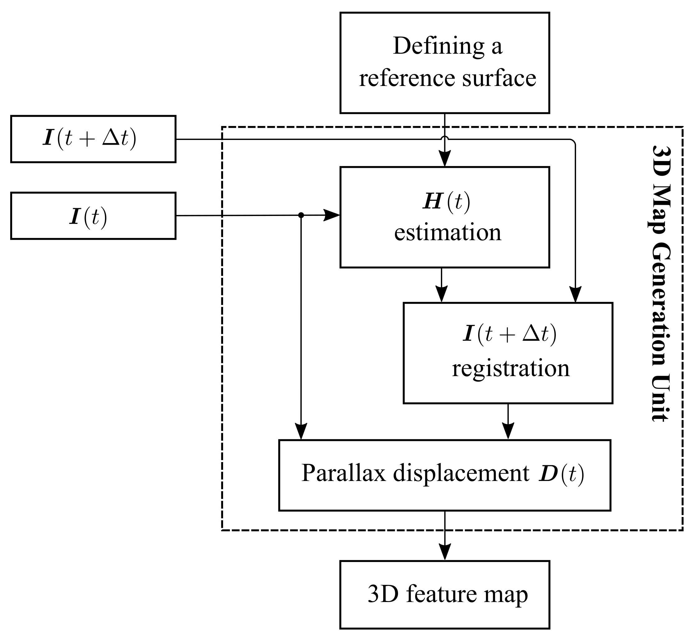
2.1. 3D Map Generation Unit

In this section, the 3D feature map generation using a pair of aerial images is described (see Figure 1). This approach utilizes a pinhole camera model [23] in which light is envisioned from the scene entering the camera from a pinhole. This results in only one ray from any particular point in the scene being projected on the image plane. Therefore, points at various heights from the ground appear on the same image plane with the camera. Upon movement of the camera, the same points appear again on the image plane but with different positions. For simplicity, it can be assumed that the reference surface is on the ground in the physical world and the image planes are parallel to the ground (see Figure 2).

In addition, ground sampling distance ($GSD$) (m/px) can be defined as the relation between scene coverage at the reference surface, S, and the image width as

$$\begin{array}{c}\hfill GSD=\frac{l}{w}=2\frac{h_{UAV}}{w}tan\left(\frac{\alpha }{2}\right)\end{array}$$

(1)

where l (m) is the scene coverage, w (px) is the image width, $h_{UAV}$ (m) is the camera’s height from the ground, and $\alpha$ is the camera’s field of view [24].

The points that were located initially beyond (or below) the reference surface in the physical world will not appear at aligned positions even after projective mapping. This discrepancy is directly proportional to the height of the point from the reference surface in the physical world. Let S be the reference surface, $\mathit{Q}$ a point above the surface, $\mathit{G}$ its projection on the surface, and $\mathit{O}$ and ${\mathit{O}}^{\prime }$ the center of projections for the two images $\mathit{I}\left(t\right)$ and $\mathit{I}(t+\Delta t)$ as portrayed in Figure 3. The projections of $\mathit{Q}$ and $\mathit{G}$ on $\mathit{I}\left(t\right)$ are $\mathit{q}$ and $\mathit{g}$, and their projections on $\mathit{I}(t+\Delta t)$ are ${\mathit{q}}^{\prime }$ and ${\mathit{g}}^{\prime }$, respectively. Furthermore, let $\mathit{M}$ and $\mathit{N}$ be the points that rays $\mathit{OQ}$ and ${\mathit{O}}^{\prime }\mathit{Q}$ intersect the surface, S. After projective mapping, points $\mathit{g}$ and ${\mathit{g}}^{\prime }$ are aligned, while the residual parallax vector, $\overrightarrow{{\mathit{qq}}^{\prime }}$, remains non-zero. The following relation is obtained considering the similar triangles of $▵\mathit{QMN}$ and $▵{\mathit{QOO}}^{\prime }$.

$$\begin{array}{c}\hfill \frac{\parallel \overrightarrow{\mathit{MN}}\parallel }{\parallel \overrightarrow{{\mathit{OO}}^{\prime }}\parallel }=\frac{h_Q}{h_{UAV}-h_Q}\end{array}$$

(2)

where $h_Q$ (m) and $h_{UAV}$ (m) are the distance between $\mathit{Q}$ and $\mathit{O}$ to the surface, S, respectively. The parallax displacement of $\overrightarrow{{\mathit{qq}}^{\prime }}$ is proportional to the physical displacement, $\overrightarrow{\mathit{MN}}$, based on $GSD$ (m/px). In addition, the physical displacement, $\overrightarrow{{\mathit{OO}}^{\prime }}$, is equal to the traveled distance of the drone with the constant speed, $v_{UAV}$ (m/s), and the sampling interval T (s). Thus, we can rewrite the previous equation and organize it according to $h_Q$ (m) as

$$\begin{array}{c}\hfill h_Q=\frac{GSD·h_{UAV}·d}{GSD·d+v_{UAV}·T}\end{array}$$

(3)

where d (px) is the parallax displacement in pixels between $\mathit{q}$ and ${\mathit{q}}^{\prime }$ ($\parallel \overrightarrow{{\mathit{qq}}^{\prime }}\parallel$). It should be noted that $(v_{UAV}·T)$ in the earlier equation can be expressed as the drone traveled distance between samplings in the case of various speed of the drone.

2.1.1. Image Registration

The pair of images ($\mathit{I}\left(t\right)$ and $\mathit{I}(t+\Delta t)$) have slightly different viewpoints, and therefore image registration is required. The different viewpoints are obtained by the displacement of the drone traveling parallel to the ground at a constant speed, $v_{UAV}$ (m/s), with a sampling time of T (s). It can be assumed the speed of the drone, $v_{UAV}$ (m/s), is known and constant, so then the sampling time, T (s), is computed based on $h_{min}$ (m), the minimum height of the objects that are supposed to be detected,

$$\begin{array}{c}\hfill T=\frac{GSD·d·(h_{UAV}-h_{min})}{v_{UAV}·h_{min}}·\end{array}$$

(4)

Equation (4) is derived from Equation (3), which takes into account that a successful 3D point detection (any point above the reference surface) requires at least one pixel parallax displacement between corresponding points ($d=1$ px). According to Equations (3) and (4), theoretically there is an inverse relationship between the sampling time and the minimum detection height for the given speed and height of the drone. Thus, it affects the accuracy of the 3D feature map of a scene. The obtained pair of aerial images are then aligned using a projective mapping.

A projective mapping is a linear transformation from one preferred plane in the first image to the same plane in the second image. Thus, the points on the reference surface in two images are aligned together. This mapping can be expressed in terms of matrix multiplications using homogeneous coordinates and a transformation matrix, $\mathit{H}\left(t\right)$ [25],

$$\begin{array}{c}\hfill \left[\begin{array}{c}x\left(t\right)\\ y\left(t\right)\\ 1\end{array}\right]=\left[\begin{array}{ccc}{h}_{11}& h_{12}& h_{13}\\ h_{21}& h_{22}& h_{23}\\ h_{31}& h_{32}& h_{33}\end{array}\right]\left[\begin{array}{c}{x}^{\prime }(t+\Delta t)\\ y^{\prime }(t+\Delta t)\\ 1\end{array}\right]=\mathit{H}\left(t\right)\left[\begin{array}{c}{x}^{\prime }(t+\Delta t)\\ y^{\prime }(t+\Delta t)\\ 1\end{array}\right],\end{array}$$

(5)

where $\left(x\right(t),y(t\left)\right)$ and $(x^{\prime }(t+\Delta t),y^{\prime }(t+\Delta t))$ are coordinates of corresponding points on the reference surface and $\mathit{H}\left(t\right)$ is a non-singular $3\times 3$ matrix. The main application of the proposed system is change detection for transportation surveillance systems such as at parking spaces in a harbor area. Therefore, the reference surface is considered on the ground/road in order to simplify the detection process of changed regions at other instants.

In this analysis, $\mathit{H}\left(t\right)$ is computed using four corresponding points on each image as only the ratio of the elements of this matrix is significant [23]. Alternatively, in order to estimate $\mathit{H}\left(t\right)$, the keypoints on the reference surface in images with variant viewpoints can be extracted based on a feature detector and descriptor, such as scale-invariant feature transform (SIFT) [26]. The detected keypoints in two images should then be matched by finding the nearest descriptors to each other using the fast-approximate nearest-neighbors (FLANN) algorithm [27].

The computed transformation matrix, $\mathit{H}\left(t\right)$, contains rotation and translation to relate the selected planes in the pair of aerial images ($\mathit{I}\left(t\right)$ and $\mathit{I}(t+\Delta t)$), and thus $\mathit{H}\left(t\right)$ is applied to all pixels on $\mathit{I}(t+\Delta t)$. For a constant sampling time, T, the transformation matrix, $\mathit{H}\left(t\right)$, is required to be computed only once as the relative positions of the two image planes remain the same.

As discussed earlier, if two arbitrary views of the same scene are registered as all points on the reference surface to be aligned, the residual parallax displacement can be used to estimate the height of any point of the image. If the aligned surface is a plane, then the parallax displacement is directly proportional to the height of the point and inversely proportional to its depth from the camera [28].

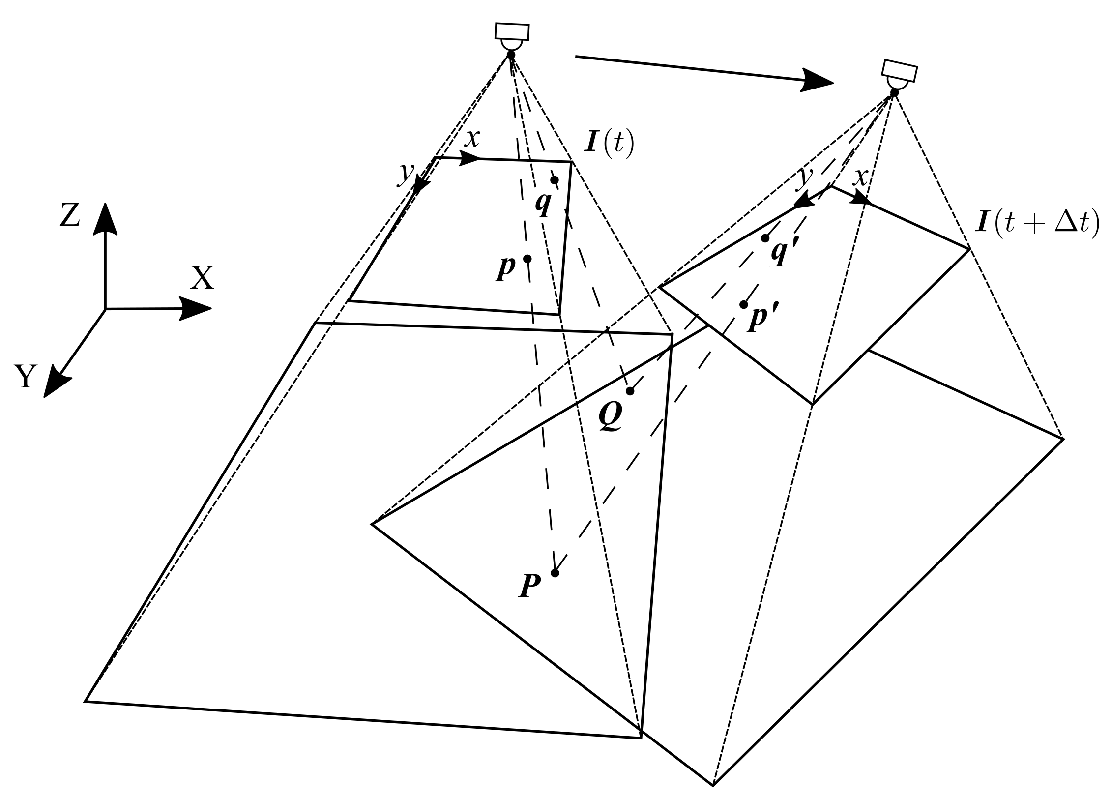
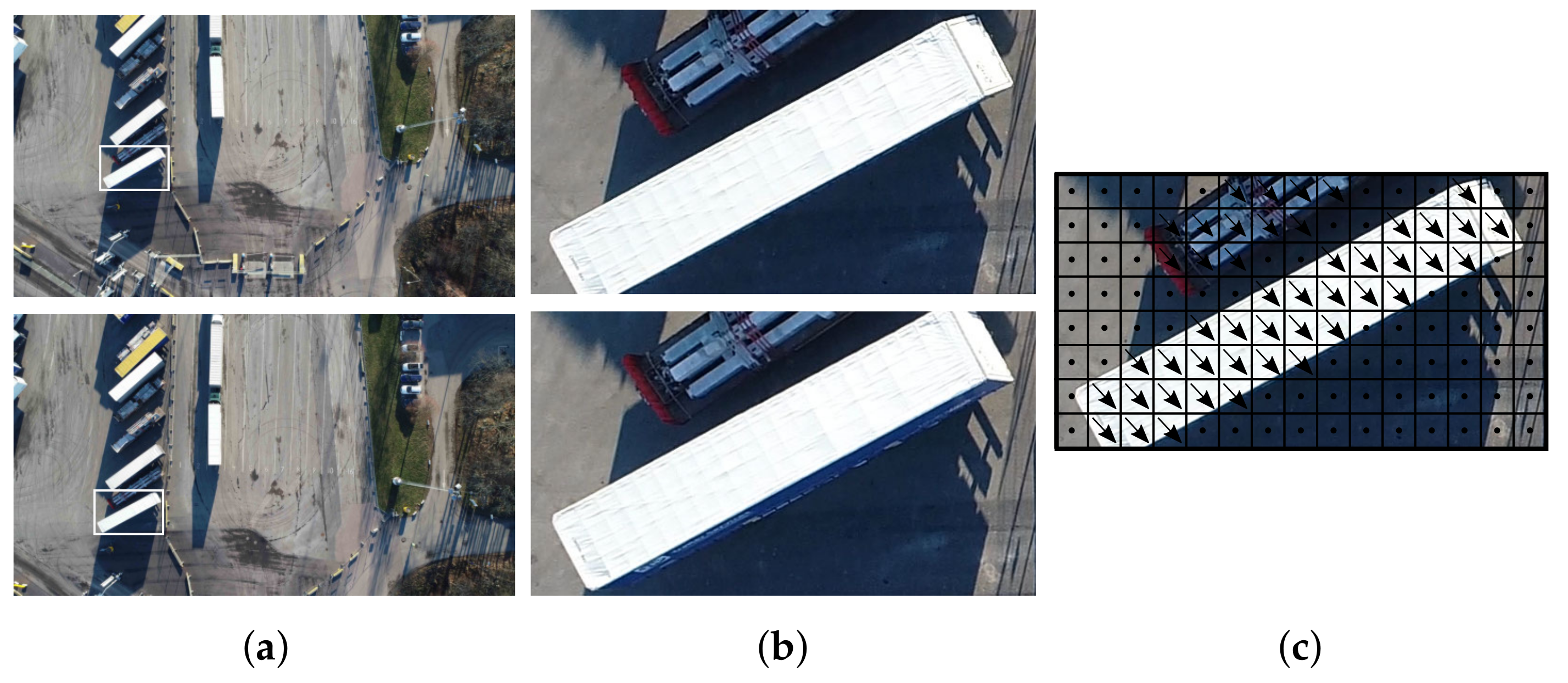
2.1.2. Parallax Displacement $\mathit{D}\left(t\right)$

The parallax displacement, $\mathit{D}\left(t\right)$, of the aerial image for all pixels should be computed in order to determine the height of each point using (3). In theory, the parallax displacement for each pixel is the Euclidean distance between $\left(x\right(t),y(t\left)\right)$ and $(x^{\prime }(t+\Delta t),y^{\prime }(t+\Delta t))$ for corresponding points. However, in practice, this leads to computation of sparse pixel parallax displacements that is not adequate to describe the height of all pixels in the image. Therefore, in this paper, the parallax displacement for each pixel is estimated based on polynomial expansion [29]. This involves estimating a neighborhood of each pixel with a quadratic polynomial function in the first image. By equating the coefficients, the parallax displacement, d, for that pixel can be estimated.

In order to improve approximation and reduce noise, it is assumed that the displacement varies slowly over a neighborhood. Thus, the parallax displacement, d, is computed as a weighted average of parallax displacements over a neighborhood of M around the pixel. The final output is a matrix, $\mathit{D}\left(t\right)$, that is equal in size to the input images which describes the magnitude of the parallax displacement vectors at each pixel (see Figure 4).

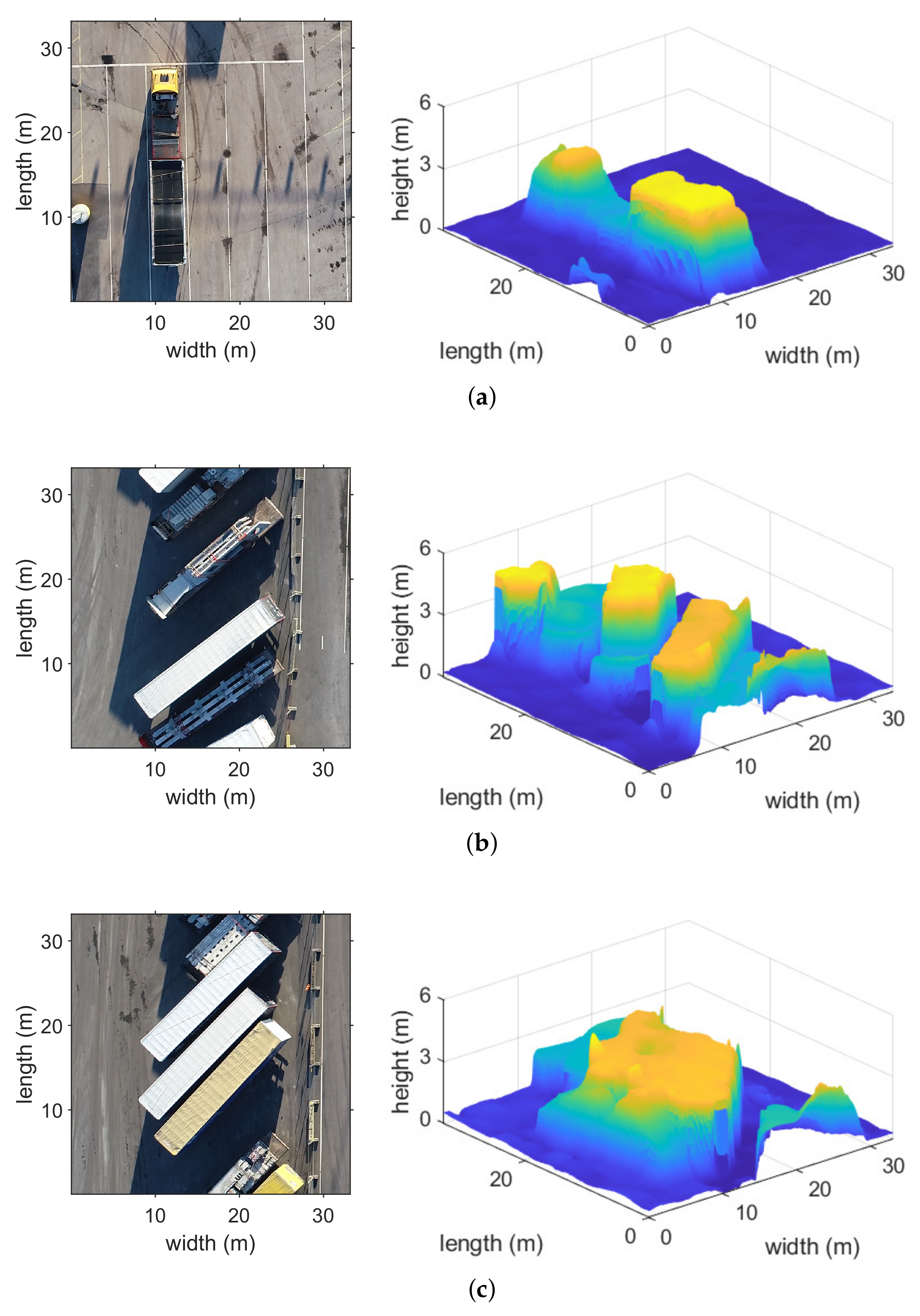
2.1.3. 3D Feature Map $\mathit{J}\left(t\right)$

The 3D feature map $\mathit{J}\left(t_1\right)$ (m) that defines the height of each pixel in the aerial image at time $t_1$ is computed based on the parallax displacements using the following equation,

$$\begin{array}{c}\hfill J_{x,y}\left(t_1\right)=\frac{GSD·D_{x,y}\left(t_1\right)·h_{UAV}}{GSD·D_{x,y}\left(t_1\right)+v_{UAV}·T}·\end{array}$$

(6)

Similarly, the second 3D feature map $\mathit{J}\left(t_2\right)$ is computed using the second pair of images, $\mathit{I}\left(t_2\right)$ and $\mathit{I}(t_2+\Delta t)$. In order to compare these 3D maps with each other, the corresponding regions should be aligned.

2.2. Change Detection Unit

After acquiring the second 3D feature map $\mathit{J}\left(t_2\right)$, the pair of 3D feature maps, $\mathit{J}\left(t_1\right)$ and $\mathit{J}\left(t_2\right)$, are compared to detect 3D point changes in the scene. The comparison model contains the height difference of corresponding pixels in two aerial images, $\mathit{I}\left(t_1\right)$ and $\mathit{I}\left(t_2\right)$. The height difference is compared with a threshold to obtain the changed regions in a scene over time (see Figure 5).

2.2.1. 3D Feature Map Registration

In order to register $\mathit{J}\left(t_2\right)$ based on $\mathit{J}\left(t_1\right)$, a projective mapping is required using the transformation matrix, $\mathit{H}(t_1,t_2)$. The transformation matrix, $\mathit{H}(t_1,t_2)$, is computed with extracted corresponding keypoints on the reference surface on $\mathit{I}\left(t_1\right)$ and $\mathit{I}\left(t_2\right)$. Subsequently, the 3D feature map $\mathit{J}\left(t_2\right)$ is warped according to $\mathit{J}\left(t_1\right)$.

2.2.2. 3D Comparison Model

The aim of the 3D comparison model is to determine the change in the height of points and consequently objects in the scene at two instants, $t_1$ and $t_2$,

$$\begin{array}{c}\hfill \mathit{E}={\mathit{J}}^{\prime }\left(t_2\right)-\mathit{J}\left(t_1\right)\end{array}$$

(7)

where ${\mathit{J}}^{\prime }\left(t_2\right)$ is the transformed 3D feature map $\mathit{J}\left(t_2\right)$.

2.2.3. Change Detection Model

The difference is considered significant if it is greater than a predefined threshold, and therefore a change in the pixel is detected,

$$\begin{array}{c}\hfill C_{x,y}=\left\{\begin{array}{cc}1,\hfill & E_{x,y}>\tau \hfill \\ 0,\hfill & \mathrm{otherwise}\hfill \end{array}\right.\end{array}$$

(8)

where $\tau$ is the predefined threshold based on the specific application.

3. Experimental Results and Discussion

Data were collected at 10 locations over two days using a commercial UAV with a built-in camera. The height of the flights was $h_{UAV}=100$ m, the camera’s field of view was $\alpha ={84}^{\circ }$, $GSD\approx 0.039$ m/px, and the image size was $3840\times 2160$ px. The respective covered area on the ground in each aerial image was approximately 150 m $\times 84$ m. The ground truth of the measurement was obtained manually, representing pixels in the image that are above the reference surface in order to evaluate the detected changes. In addition, the results were compared using an adaptive model known as Kendall’s Tau-d local pattern correlation with the intensity similarity threshold, $\mathit{alpha}=0.7$, and the texture similarity threshold, $\mathit{beta}=0.95$ [30].

The objective of the proposed system was to extract the height information of the pixels from aerial images taken at different times and, consequently, to compare the extracted 3D feature maps in order to determine regions with significant changes in their height profiles. The sampling time is computed to be $T=2.3$ s using (6) by setting the drone speed, $v_{UAV}=4.8$ m/s, and the minimum height of the objects, $h_{min}=0.42$ m.

The evaluation parameters to assess the performance of the proposed change detection system are the accuracy rate (ACC), the true positive rate (TPR), and the false positive rate (FPR).

$$\begin{array}{c}\hfill ACC=\frac{TP+TN}{TP+TN+FP+FN}\end{array}$$

(9)

$$\begin{array}{c}\hfill TPR=\frac{TP}{TP+FN}\end{array}$$

(10)

$$\begin{array}{c}\hfill FPR=\frac{FP}{FP+TN}\end{array}$$

(11)

where $TP$, $FP$, $TN$, and $FN$ are true positive, false positive, true negative, and false negative, respectively.

The robustness and accuracy of the proposed system is closely related to the detection of parallax displacements. Therefore, one of the main parameters that impacts performance is the size of the neighborhood, M, around pixels where the weighted average of parallax displacements is computed. This is particularly important as not all pixels contain dominant keypoints, and thus displacements at those pixels are not reliable [29]. A suitable size for the neighborhood window depends on shape and size of the objects in the scene. In this paper, variant neighborhood window sizes are employed and 3D feature maps are compared against their ground truth. The results are displayed using a receiver operating characteristic (ROC) curve in Figure 6. In this context, positive is considered a pixel above and negative a pixel on the reference surface. Accordingly, the performance of the proposed model with respect to the 3D feature map extraction for variant neighborhood window sizes, M, is presented by the true positive rate and false positive rate computed using Equations (10) and (11).

Based on the obtained ROC curve, the neighborhood window size is set to $M=40$ and $M=50$ and the 3D feature maps are generated for 10 locations over two days. The experimental results are discussed with examples from aerial images in different scenarios in order to evaluate the performance of the proposed model more specifically (see Figure 7).

In the first scenario, a single object, a truck trailer, is observed on a sunny day with strong shadows standing alone in the scene (see Figure 7a). The generated 3D feature map of the scene accurately corresponds to the object and its surroundings. Even the variant height of the trailer section and the wind deflector on the cabin are reflected accurately in the 3D map. The second scenario considers multiple objects in the scene (see Figure 7b). In this case, several trailers with variant heights are located beside each other with strong shadows covering them partially. The generated 3D feature map corresponds to each trailer individually with correct height reconstruction of the scene. The third scenario involves multiple objects with little space in between (see Figure 7c). In this case, the dense objects are reconstructed correctly, and variant heights as well as corresponding covered areas are generated accordingly in the 3D feature map. These results demonstrate the performance of the proposed model under various scenarios using only a pair of aerial images.

The analysed surfaces in focus for change detection in this work were mainly vehicles and trailers in a harbour area as for transportation applications. In addition, it was observed that construction of 3D feature maps from homogeneous surfaces (areas with a uniform appearance, e.g., a truck trailer’s roof) raised difficulty due to having less distinctive keypoints [31]. Thus, as mentioned earlier, the parallax displacement was computed over a neighborhood window, M, in order to compensate for the lack of distinctive keypoints. As a result, the obtained 3D feature maps were more reliable especially for homogeneous surfaces; however, it introduced some errors over the edges. Moreover, the proposed method can potentially be applied for more complex surfaces such as hilly and even urban areas as we have partially observed in the experimental results.

It is worth mentioning that there are available commercial algorithms in order to achieve 3D reconstruction of a scene [32,33]. However, the main goal of the proposed method is to perform change detection in a scene by utilizing 3D feature maps. Moreover, the 3D feature map is acquired using only one pair of aerial images rather than several. The precision of the 3D feature maps might be compromised while it is computationally highly efficient to detect changed regions over large areas.

The aligned 3D feature maps are then compared, and regions with significant changes are detected and compared against the ground truth. In addition, regions with similar heights but above the reference surface are also marked. This information is particularly important when studying the utilization of the scene in the physical world. Figure 8 illustrates change detection examples for three regions on two different days using the corresponding generated 3D feature maps. In the first and second regions, vans have disappeared on the second day; therefore, there are changes in the respective scenes over time. However, in the second region the vehicle’s color was very similar to the background that makes it more difficult for the conventional change detection methods. In the third region, several trailers have been replaced with some other trailers with variant heights, positions and colors in a more challenging scenario. The absolute difference in the corresponding pixel heights successfully establishes the amount of detected changes in the respective regions for all three scenarios (see Figure 8c,f,i).

Table 1. The performance evaluation of the proposed model and Kendall’s Tau-d model.

Comparison Model	FPR (%)	TPR (%)	ACC (%)
Kendall’s Tau-d model	19.49	57.07	73.11
with $\mathit{alpha}=\mathbf{0.7}$ and $\mathit{beta}=\mathbf{0.95}$
3D model with $\mathbf{M}=\mathbf{40}$	17.89	88.65	84.17
3D model with $\mathbf{M}=\mathbf{50}$	22.21	92.93	82.56

demonstrates the change detection results over two days using the proposed system on 10 pairs of aerial images on each day. The smallest observed objects were passenger vehicles approximately $2m$ by $4m$ with a height of $1.5m$. In order to compare the results of the proposed system with another model, a local pattern correlation descriptor called Kendall’s Tau-d is implemented and the obtained results are presented. The change detection results using the proposed 3D change detection approach are more accurate than those obtained using the intensity model. The main reason for this is that any intensity comparison model is highly dependent on brightness and illumination within two different instances of time. In contrast, the proposed 3D comparison model is affected by brightness conditions only at nearly the same time to construct a 3D feature map and the comparison of the 3D feature maps can accommodate changes in illumination. Moreover, the amount of noise in the image based on reflection (e.g., having a wet surface), strong shadows, and other factors can be very high at two different times, potentially affecting intensity methods negatively. Furthermore, intensity comparison methods cannot distinguish between objects with similar patterns and colors (e.g., white trailers in aerial images), meaning they fail to detect changes. On the contrary, the proposed 3D model features height information of objects in the scene at both instants.

The computation time of the presented method can be considered in two parts: first, to create the 3D feature maps and second to detect changes using the obtained 3D feature maps. The computation time of the first part for creating the 3D feature map at each instant from a pair of aerial images with sizes of $3840\times 2160$ px was approximately $1.76$ s. Then, it took ~$0.06$ s to compute the changed regions in a scene for the second part. In comparison, a well-known commercial software [32] was used to create the 3D feature map with the same pair of aerial images and giving four pair of corresponding keypoints to define the reference surface. The total computation time of the software to perform this task was approximately $28.32$ s that includes aligning the images, building the dense cloud, and finally building the mesh. Furthermore, the Kendall’s Tau-d model [30] determined changes in aerial images over time in ~$33.03$ s (non-vectorized implementation). These computation times show a significant improvement in the processing time and, consequently, the computational cost as the result of the proposed method.

In addition, the proposed method can be used to detect 3D objects with respect to the reference surface in oblique aerial images (see the Section 5). However, in the case of oblique images (in contrast to orthogonal aerial images), perspective distortion causes significant depth variation. Nevertheless, using the described method, the relative position of any pixel to the reference surface can be determined so that 3D objects can be detected in the scene.

4. Conclusions

Change detection in multitemporal aerial images is challenging because of variant brightness, shadows, colors, and surface conditions at two or more instants. The proposed method in this paper determines changes in the scene regardless of the aforementioned undesired conditions. This method is based on height extraction of each point in the aerial images of a scene. The height information is computed using the parallax displacements and then related to the actual distance from the reference surface in the physical world. Consequently, the computed 3D feature maps are aligned and compared at different times to detect changes in the scene. The experimental results show that the proposed system effectively detects changed regions in the scene with an accuracy rate and true positive rate of $82.56$% and $92.93$%, respectively. Furthermore, this method is able to accommodate changes in illumination, strong shadows, and noise at different instants. In addition, a mathematical model is presented to calculate the suitable image sampling rate based on the minimum height of interest. It can be concluded that the proposed method determines changed regions in multitemporal aerial images quickly, efficiently, and with relatively low computational cost as an alternative to conventional intensity and pattern correlation comparison models.

5. Patent

Pettersson, M.I.; Javadi, S.; Dahl, M. A method for detecting changes of objects in a Scene. Swedish Patent 1850695-6, filed 8 June 2018, and expected to be issued 1 May 2020.

References

1. Zhan, Y.; Fu, K.; Yan, M.; Sun, X.; Wang, H.; Qiu, X. Change detection based on deep siamese convolutional network for optical aerial images. IEEE Geosci. Remote Sens. Lett. 2017, 14, 1845–1849. [Google Scholar] [CrossRef]
2. Ali-Sisto, D.; Packalen, P. Forest change detection by using point clouds from dense image matching together with a liDAR-derived terrain model. IEEE J. Sel. Top. Appl. Earth Obs. Remote Sens. 2017, 10, 1197–1206. [Google Scholar] [CrossRef]
3. Jordan, S.; Moore, J.; Hovet, S.; Box, J.; Perry, J.; Kirsche, K.; Lewis, D.; Tse, Z. State-of-the-art technologies for UAV inspections. IET Radar Sonar Navig. 2018, 12, 151–164. [Google Scholar] [CrossRef]
4. Yan, J.; Peng, Z.; Hong, H.; Chu, H.; Zhu, X.; Li, C. Vital-SAR-imaging with a drone-based hybrid radar system. IEEE Trans. Microw. Theory Tech. 2018, 66, 5852–5862. [Google Scholar] [CrossRef]
5. Bazi, Y.; Melgani, F. Convolutional SVM networks for object detection in UAV imagery. IEEE Trans. Geosci. Remote Sens. 2018, 56, 3107–3118. [Google Scholar] [CrossRef]
6. Stockdale, C.A.; Bozzini, C.; Macdonald, S.E.; Higgs, E. Extracting ecological information from oblique angle terrestrial landscape photographs: Performance evaluation of the WSL monoplotting tool. Appl. Geogr. 2015, 63, 315–325. [Google Scholar] [CrossRef]
7. Song, F.; Dan, T.; Yu, R.; Yang, K.; Tang, Y.; Chen, W.; Gao, X.; Ong, S. Small UAV-based multi-temporal change detection for monitoring cultivated land cover changes in mountainous terrain. Remote Sens. Lett. 2019, 10, 573–582. [Google Scholar] [CrossRef]
8. Celik, T. Unsupervised change detection in satellite images using principal component analysis and k-means clustering. IEEE Geosci. Remote Sens. Lett. 2009, 6, 772–776. [Google Scholar] [CrossRef]
9. Benedek, C.; Szirányi, T. Change detection in optical aerial images by a multilayer conditional mixed Markov model. IEEE Trans. Geosci. Remote Sens. 2009, 47, 3416–3430. [Google Scholar] [CrossRef] [Green Version]
10. Singh, P.; Kato, Z.; Zerubia, J. A multilayer Markovian model for change detection in aerial image pairs with large time differences. In Proceedings of the 2014 22nd International Conference on Pattern Recognition, Stockholm, Sweden, 24–28 August 2014; pp. 924–929. [Google Scholar] [CrossRef] [Green Version]
11. Liu, J.; Gong, M.; Qin, K.; Zhang, P. A deep convolutional coupling network for change detection based on heterogeneous optical and radar images. IEEE Trans. Neural Netw. Learn. Syst. 2018, 29, 545–559. [Google Scholar] [CrossRef] [PubMed]
12. Ma, W.; Yang, H.; Wu, Y.; Xiong, Y.; Hu, T.; Jiao, L.; Hou, B. Change Detection Based on Multi-Grained Cascade Forest and Multi-Scale Fusion for SAR Images. Remote Sens. 2019, 11, 142. [Google Scholar] [CrossRef] [Green Version]
13. Hirschmuller, H. Stereo processing by semiglobal matching and mutual information. IEEE Trans. Pattern Anal. Mach. Intell. 2008, 30, 328–341. [Google Scholar] [CrossRef] [PubMed]
14. Zang, Y.; Yang, B.; Li, J.; Guan, H. An accurate TLS and UAV image point clouds registration method for deformation detection of chaotic hillside areas. Remote Sens. 2019, 11, 647. [Google Scholar] [CrossRef] [Green Version]
15. James, M.R.; Robson, S.; Smith, M.W. 3-D uncertainty-based topographic change detection with structure-from-motion photogrammetry: Precision maps for ground control and directly georeferenced surveys. Earth Surf. Process. Landf. 2017, 42, 1769–1788. [Google Scholar] [CrossRef]
16. Barber, D.M.; Holland, D.; Mills, J.P. Change detection for topographic mapping using threedimensional data structures. Int. Arch. Photogramm. Remote Sens. Spat. Inf. Sci. 2008, 37, 1177–1182. [Google Scholar]
17. Alcantarilla, P.F.; Stent, S.; Ros, G.; Gherardi, R. Street-view change detection with deconvolutional networks. Auton. Robot. 2018, 42, 1301–1322. [Google Scholar] [CrossRef]
18. Chen, B.; Deng, L.; Duan, Y.; Huang, S.; Zhou, J. Building change detection based on 3D reconstruction. In Proceedings of the IEEE International Conference on Image Processing (ICIP), Quebec City, QC, Canada, 27–30 September 2015; pp. 4126–4130. [Google Scholar] [CrossRef]
19. Finman, R.; Whelan, T.; Kaess, M.; Leonard, J.J. Toward lifelong object segmentation from change detection in dense RGB-D maps. In Proceedings of the European Conference on Mobile Robots, Barcelona, Spain, 25–27 September 2013; pp. 178–185. [Google Scholar] [CrossRef] [Green Version]
20. Kahn, S.; Bockholt, U.; Kuijper, A.; Fellner, D.W. Towards precise real-time 3D difference detection for industrial applications. Comput. Ind. 2013, 64, 1115–1128. [Google Scholar] [CrossRef]
21. Sharifzadeh, S.; Baharlou, S.M.; Berrendorf, M.; Koner, R.; Tresp, V. Improving visual relation detection using depth maps. arXiv 2019, arXiv:1905.00966. [Google Scholar]
22. Tyagi, A.; Drinkard, J.; Tani, Y.; Kinoshita, K. Method and Apparatus for Projective Volume Monitoring. U.S. Patent US20160203371A1, 14 July 2016. [Google Scholar]
23. Kaehler, A.; Bradski, G. Camera models and calibration. In Learning OpenCV 3: Computer Vision in C++ with the OpenCV Library, 1st ed.; O’Reilly Media Inc.: Newton, MA, USA, 2016; pp. 637–664. [Google Scholar]
24. Rumpler, M.; Tscharf, A.; Mostegel, C.; Daftry, S.; Hoppe, C.; Prettenthaler, R.; Fraundorfer, F.; Mayer, G.; Bischof, H. Evaluations on multi-scale camera networks for precise and geo-accurate reconstructions from aerial and terrestrial images with user guidance. Comput. Vis. Image Underst. 2017, 157, 255–273. [Google Scholar] [CrossRef] [Green Version]
25. Hartley, R.; Zisserman, A. Pojective geometry and transformations of 2D. In Multiple View Geometry in Computer Vision, 2nd ed.; Cambridge University Press: Cambridge, MA, USA, 2003; pp. 32–37. [Google Scholar]
26. Lowe, D.G. Object recognition from local scale-invariant features. In Proceedings of the 7th IEEE International Conference on Computer Vision, Kerkyra, Greece, 20–25 September 1999; pp. 1150–1157. [Google Scholar] [CrossRef]
27. Muja, M.; Lowe, D.G. Fast approximate nearest neighbors with automatic algorithm configuration. In Proceedings of the International Conference Computer Vision Theory and Applications, Lisboa, Portugal, 5–8 February 2009; pp. 331–340. [Google Scholar]
28. Kumar, R.; Anandan, P.; Hanna, K. Direct recovery of shape from multiple views: A parallax based approach. In Proceedings of the 12th IAPR International Conference on Pattern Recognition—Conference A: Computer Vision & Image Processing, Jerusalem, Israel, 9–13 October 1994; pp. 685–688. [Google Scholar] [CrossRef]
29. Farnebäck, G. Two-frame motion estimation based on polynomial expansion. In Proceedings of the 13th Scandinavian Conference on Image Analysis, Halmstad, Sweden, 29 June–2 July 2003; pp. 363–370. [Google Scholar] [CrossRef] [Green Version]
30. Javadi, S.; Dahl, M.; Pettersson, M.I. Change detection in aerial images using a Kendall’s TAU distance pattern correlation. In Proceedings of the 2016 6th European Workshop on Visual Information Processing (EUVIP), Marseille, France, 25–27 October 2016; pp. 1–6. [Google Scholar] [CrossRef]
31. Popielski, P.; Wróbel, Z. The feature detection on the homogeneous surfaces with projected pattern. In Information Technologies in Biomedicine. Lecture Notes in Computer Science; Piętka, E., Kawa, J., Eds.; Springer: Berlin/Heidelberg, Germany, 2012; pp. 118–128. [Google Scholar] [CrossRef]
32. Agisoft Metashape. Available online: https://www.agisoft.com (accessed on 7 April 2020).
33. Pix4Dmapper. Available online: https://www.pix4d.com (accessed on 7 April 2020).
Figure 1. The 3D feature map of a scene using a pair of aerial images.
Remotesensing 12 01404 g001
Figure 2. A pair of aerial images, I ( t ) and I ( t + Δ t ) (the camera’s image planes). Point P is considered to be on the reference surface and point Q above it. The projections of these points on their respective image planes are shown as p and q on I ( t ) and p , and q on I ( t + Δ t ) .
Remotesensing 12 01404 g002
Figure 3. The projective planes of I ( t ) and I ( t + Δ t ) taken at height h U A V above the ground with the centre of projections at O and O , respectively, observing a point at Q at the height h Q above the ground.
Remotesensing 12 01404 g003
Figure 4. Parallax displacement calculation: (a) a pair of aerial images; (b) region of interest in both images after alignment based on the reference surface; (c) vector of parallax displacement for each pixel where its magnitude is considered D ( t ) .
Remotesensing 12 01404 g004
Figure 5. The 3D comparison and change detection models based on the 3D feature maps.
Remotesensing 12 01404 g005
Figure 6. The receiver operating characteristic (ROC) curve for variant neighborhood window sizes, 5 M 125 , and their performance.
Remotesensing 12 01404 g006
Figure 7. Examples of generated 3D feature maps under different scenarios: (a) single object; (b) multiple objects; (c) dense multiple objects.
Remotesensing 12 01404 g007
Figure 8. Change detection in three regions using generated 3D feature maps: (a,d,g) day 1; (b,e,h) day 2; (c,f,i) 3D comparison model E showing the differences in height properties of the respective scenes.
Remotesensing 12 01404 g008