Article

An Optimal Troposphere Tomography Technique Using the WRF Model Outputs and Topography of the Area

1
Faculty of Civil Engineering and Geosciences, Delft University of Technology, Stevinweg 1, 2628 CN Delft, The Netherlands
2
Faculty of Geodesy and Geomatics Engineering, K. N. Toosi University of Technology, Tehran 15433-19967, Iran
3
Institute of Geodesy and Geoinformatics Wroclaw, University of Environmental and Life Sciences, Grunwaldzka 53, 50-357 Wroclaw, Poland
*
Author to whom correspondence should be addressed.
Remote Sens. 2020, 12(9), 1442; https://doi.org/10.3390/rs12091442
Submission received: 20 March 2020 / Revised: 29 April 2020 / Accepted: 30 April 2020 / Published: 2 May 2020
(This article belongs to the Section Atmospheric Remote Sensing)

Abstract

:
The water vapor content in the atmosphere can be reconstructed using the all-weather condition troposphere tomography technique. In common troposphere tomography, the water vapor of each voxel is represented by an unknown parameter. This means that when the desired spatial resolution is high or study area is large, there will be a huge number of unknown parameters in the problem that need to be solved. This defect can reduce the accuracy of troposphere tomography results. In order to overcome this problem, an optimal voxel-based troposphere tomography using the Weather Research and Forecasting (WRF) model is proposed. The new approach reduces the number of unknown parameters, the number of empty voxels and the role of constraints required to enhance the spatial resolution of tomography results in required areas. Furthermore, the effect of considering the topography of the study area in the tomography model is examined. The obtained water vapor is validated by radiosonde observations and Global Positioning System (GPS) positioning results. Comparison of the results with the radiosonde observations shows that using the WRF model outputs and topography of the area can reduce the Root Mean Square Error (RMSE) by 0.803 gr/m3. Validation using positioning shows that in wet weather conditions, the WRF model outputs and topography reduce the RMSE of the east, north and up components by about 17.42, 10.46 and 20.03 mm, which are equivalent to 46.01%, 35.78% and 53.93%, respectively.

1. Introduction

The accurate reconstruction of water vapor is very important for weather forecasting and other applications, such as the early warning of weather disasters. There are many instruments all over the world for measuring water vapor, such as meteorological sensors on in space, air and ground -based platforms, but they all have provide low spatiotemporal resolution and have high costs [1,2]. The troposphere tomography technique is nowadays known as one of the most powerful and accurate methods for the three-dimensional (3D) reconstruction of water vapor. The troposphere tomography technique has been investigated for the first time by Flores et al. (2000) and Hirahara (2000) [3,4]. Tomography is a powerful technique for the reconstruction of atmospheric layers, especially the troposphere and the ionosphere [5]. Tropospheric tomography is generally performed using the voxel-based method. Many researchers have tried to improve the accuracy of the results by optimizing different aspects of the voxel-based troposphere tomography: (1) improving the inversion process [6,7], (2) reformatting the model geometry [8,9,10,11,12], (3) applying advance optimization techniques [13], (4) using the signals penetrating into the side face of the tomography model and using the data from Global Navigation Satellites System (GNSS) observations outside the study region [8,10,14,15,16]. An important overview of the benefits and deficiencies of current tomography models could be found in [17]. Water vapor reconstruction using voxel-based troposphere tomography is an inverse problem. According to previous articles, the most common way to solve this problem is to use regularization methods [12]. In most of the currently used models [17] this method uses only one unknown parameter to represent the water vapor in each voxel and cannot compute the water vapor distribution within a voxel. Another issue related to model geometry is topography, which is usually not present in the voxel parametrization [7]. Therefore, the number of voxels or number of unknown parameters increases when there is a need for high spatial resolution water vapor reconstruction, which is of interest in complex terrains. Increasing the number of unknown parameters decreases the degree of freedom of the problem, decreases the accuracy of the results and may also increase the need to use constraints to solve the problem.
In this paper, to overcome the complex model geometry problem, two ideas are introduced: (1) an optimal voxel-based troposphere tomography based on the WRF model outputs, (2) precise representation of the model topography. These new ideas can increase the spatial resolution of the tomography results in required areas. This method also reduces the number of unknown parameters and the number of required constraints. The proposed method was tested using a Global Positioning System (GPS) network in North America in different weather conditions. The Global Forecast System analysis (GFS) and ERA5 data were used as inputs to the WRF model and to perform the 3D ray tracing technique, respectively. Finally, the obtained results were validated with the radiosonde measurements; also, the GPS precise point positioning technique was adopted to verify the impact of accurate troposphere tomography modelling. In the following, the basics of the voxel-based troposphere tomography and the new method are provided (Section 2). Then, the study area and data set are presented (Section 3). The obtained results and validation are presented in the last section.

2. The Principle of the Voxel-Based Troposphere Tomography

2.1. General Approach

The slant water vapor (SWV) is one of the most important indicators that can be used as an input for the troposphere tomography problem and is expressed as follows [18]:
S W V = Rec . S a t . ρ ( s ) d s     ,
where s represents the path of the ray and ρ is the water vapor density (WVD). It can be estimated using following equation [18]:
S W V = 10 R w [ ( k 3 / T m ) + k 2 ] S W D ,
where k 2 = 16.48 Khpa 1 ,   k 3 = 3.776 × 10 5 K 2 hpa 1 and R w = 461 JKg 1 K 1 are specific gas constants, Tm is the weighted mean tropospheric temperature and SWD is the slant wet delay of the ray. The SWD can be estimated using [3]:
S W D = ( m f w e t × Z W D ) + ( m f w e t × cot ( α ) × ( ( G N S W × cos φ ) + ( G E W W × sin φ ) ) ) + R ,
where mfwet is the non-hydrostatic mapping function, α is the satellite elevation, φ is the azimuth, R is the modeled residual and GNSW and GEWW are non-hydrostatic delay gradients in N-S and E-W directions. ZWD is the zenith wet delay, which can be estimated by subtracting the zenith hydrostatic delay (ZHD) from the zenith total delay (ZTD). ZTD and ZHD can be computed accurately using the Global Navigation Satellites System (GNSS) processing and empirical models, respectively [19].
In the voxel-based troposphere tomography method, the tomography area is divided into a number of voxels in which the WVD is considered as a constant during the specified period of time. Therefore, the equation between the SWV and the WVD of Equation (1) can be discretized as follows [20]:
S W V P = i m d i P   ρ i ,
where m is the number of voxels in the tomography model, P is the counter of rays, d i P is the distance travelled by the ray P in the voxel i and ρ i is the WVD in the voxel i. Equation (4) can be written in the matrix form:
L r × 1 = A r × m X m × 1 ,
where r is the number of GNSS rays, A is the coefficient matrix and X is the vector of the unknown WVD in each voxel. In order to form the coefficients matrix, it is necessary to calculate the distance traveled by the rays is each voxel. In this paper, the 3D ray tracing technique based on eikonal equations is used to calculate the distance [11,12]. The model resolution matrix is used to select the optimal resolution and geometry for the tomography model [11]. In the troposphere tomography problem, the coefficient matrix has a rank deficiency, for example because some voxels may not be passed by any ray or due to large distances between stations. To overcome this problem, the most common method is to impose constraint information. In this study, the horizontal constraint was performed based on the assumption that the WVD in a voxel is a mean value of its horizontally near neighbors [8]. In order to form the vertical constraints, the negative exponential function is used [3]. The troposphere tomography is a large and ill-conditioned inverse problem due to the high number of observations, wide area of modelling, number of intersections and the unavailability of observations from the sides of the model. Therefore, the use of regularization methods is necessary to solve the problem. In this paper, the least-squares QR (LSQR) iterative regularization method is used [11,12].
The RMSE and Pearson product-moment correlation coefficient (PCC) have been used for statistical analysis of the obtained results. The PCC is commonly used to measure the correlation between two data series [21]:
P C C = i = 1 N ( X i X i ¯ ) ( Y i Y i ¯ ) i = 1 N ( X i X i ¯ ) 2 i = 1 N ( Y i Y i ¯ ) 2 .

2.2. Optimal Approach Based on the WRF Model and Topography of the Area

The purpose of this new idea was to increase the spatial resolution of the tomography model in required areas in addition to reducing the number of unknown parameters. For this purpose, a high-resolution model for the tomography problem was considered. It was clear that in this case, due to the large number of unknown parameters, the use of a huge number of constraints was inevitable. Therefore, in the next step, before solving the problem, neighboring voxels with small differences in water vapor are merged to each other. Using this idea, the tomography results could be obtained with a high spatial resolution in areas with large water vapor variations. In order to implement this approach, the use of weather forecasting models such as WRF was inevitable. Based on the WRF model outputs at any epoch, it could be concluded which voxels could be merged before solving the tomography problem. In the following, the criteria for merging voxels is discussed. It was necessary to know how much of the water vapor variations did not have a significant effect on the GPS tropospheric wet delay and positioning results. For this aim, a sensitivity analysis was performed using meteorological data under different weather conditions and in different locations of the area. The ZWD could be obtained using following formula [18]:
Z W D = 10 6 h ( k 2 e T + k 3 e T 2 ) d h = 10 6 i ( k 2 e i T i + k 3 e i T i 2 ) Δ h ,
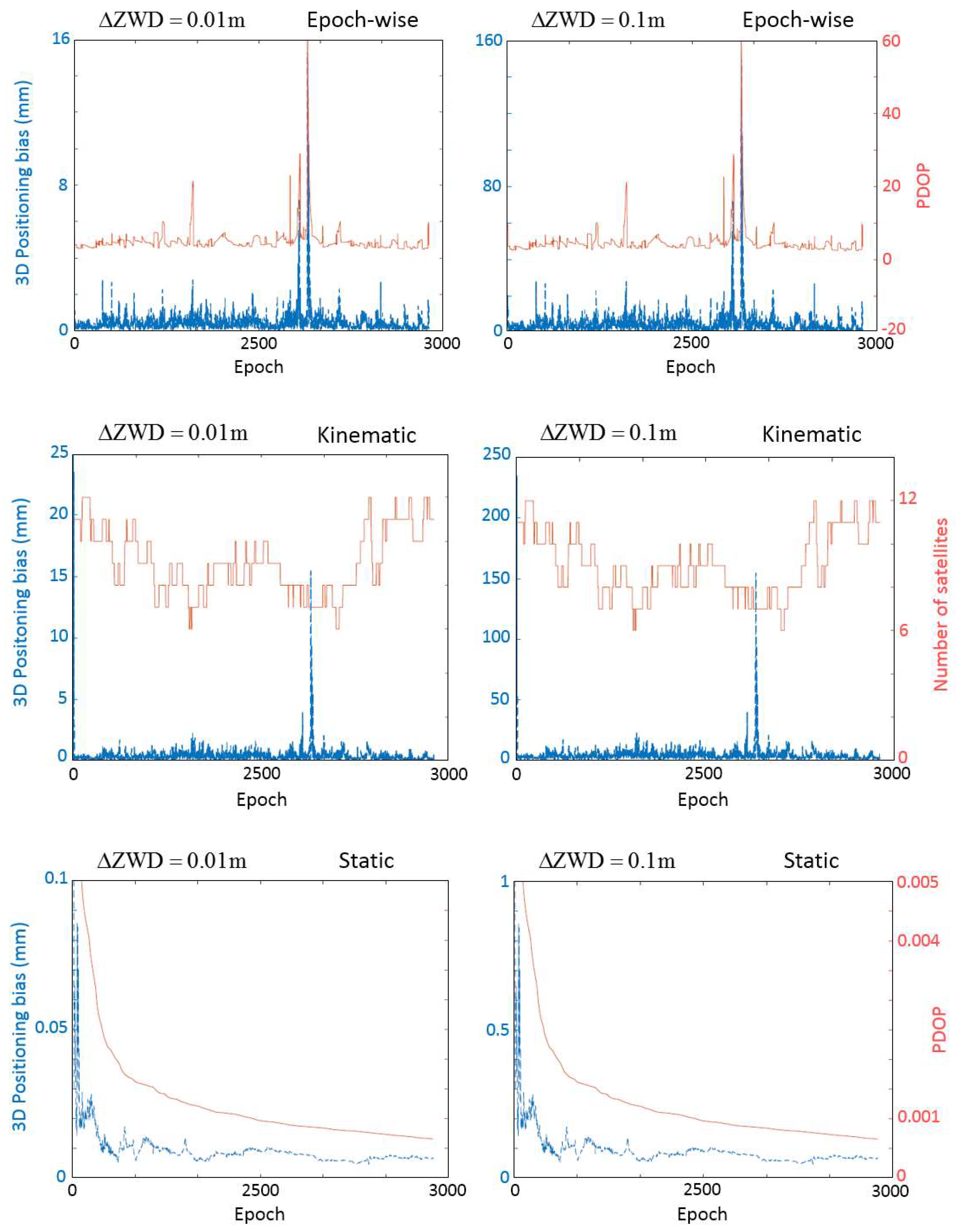
where e is the water vapor pressure (hPa), T is the temperature (K), Δ h is the thickness of the vertical layers and i is the number of layers. Based on the Equation (7), a sensitivity analysis was performed using ERA5 data. The ZWD was computed from the surface to the height of 10 km, which is a normal height for troposphere tomography models. An example of this analysis is visible in Figure 1. Based on this analysis, it can be said that one unit increase in water vapor pressure in each vertical layer causes an average increase of 12 mm in ZWD. After this step, in order to complete the sensitivity analysis, it was necessary to evaluate the effect of ZWD offsets on the positioning. This effect was investigated in three different positioning modes, including epoch-wise, kinematic and static. To investigate the impacts of the ZWD offsets on the positioning solution, a simulation was set up to verify the tolerance of the variable tropospheric delay for the positioning solution. A tightly constrained process noise was given to the tropospheric delay parameter, since both the simulation and the following real data test were in a normal weather condition. Figure 2 shows the 3D positioning bias due to the ZWD offsets ( Δ Z W D ), position dilution of precision (PDOP) and number of satellites.
Based on the Figure 2, it can be said that the ZWD offset has a direct relationship with the positioning bias. In static mode, a 10-meter offset in the tropospheric wet delay generates a bias of less than one millimeter in position. It can be concluded that the effect of the ZWD offset on the position in the kinematic mode is greater than in the other modes. According to the results presented in Figure 1 and Figure 2, a 0.8-unit change in water vapor pressure, which is a value between 0.5 and 1, is considered as a permissible limit for voxel integration. On the basis of the above mentioned, the following algorithm can be considered for this new idea (Figure 3).
As can be seen, the number of voxels that are free of radiation will be reduced if the voxels near the edge of the tomography model can be merged. Therefore, this method has three advantages. First, it reduces the number of unknown parameters. Second, the spatial resolution of the tomography results is increased in the required areas where water vapor variations are large. Third, the need to use external constraints is reduced.
In this paper, the impact of considering the topography of the area is investigated in addition to examining the effect of using the WRF model outputs. It is expected that the use of topography also reduces the number of empty voxels and required constraints and increases the accuracy of the results, similar to applying the WRF model.

3. Study Area and Data Set

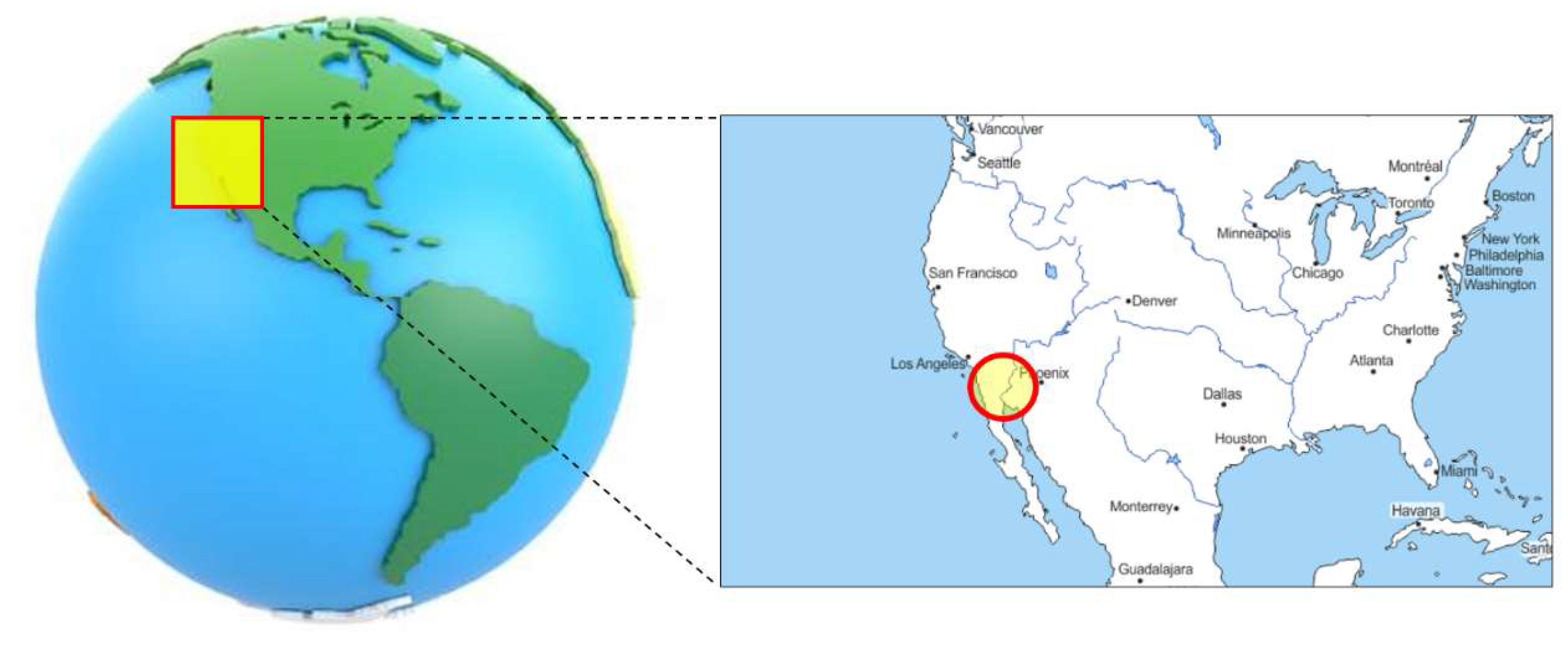
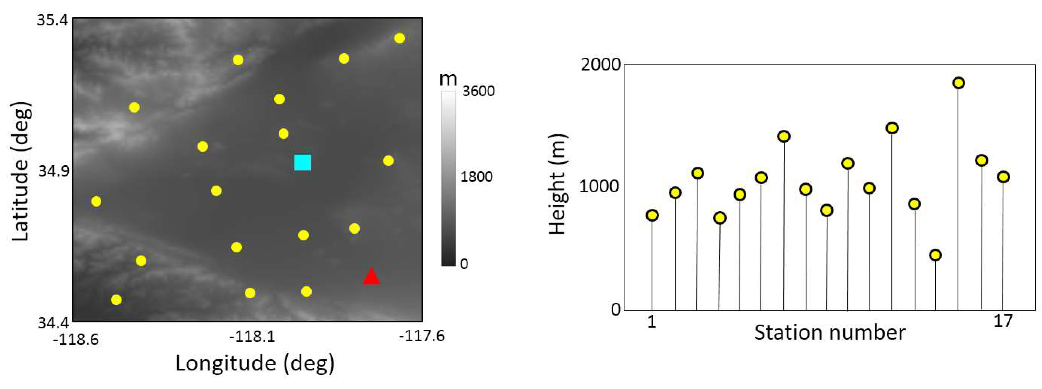
In order to implement the new idea, a region in North America was selected (Figure 4). Observations of 17 GPS stations located in this area under different weather conditions were used for this study. The distribution of the GPS stations and the topography of the study area can be seen in Figure 5. In order to obtain reliable and representative results, 10 Days of Year (DOYs) with different weather conditions were selected.
In this research, the ERA5 reanalysis data published by the European Centre for Medium-Range Weather Forecasts (ECMWF) were used to perform the 3D ray tracing technique. Previous studies have shown that this data is very useful in a variety of fields, including geodynamics and geodesy [22,23]. The ERA5 is a climate reanalysis dataset, covering the period from 1950 to the present. The ERA5 contains most parameters available in its predecessor, ERA-Interim, and ERA5 has some additional parameters. This model presented values of meteorological data on 37 pressure levels. The spatial resolution of this data was about 31 km [24].
The Global Forecast System analysis (GFS) data were used to run the WRF model and predict meteorological data. The GFS is a numerical weather forecast model presented by the National Centers for Environmental Prediction (NCEP). Many of the atmospheric and land-soil variables are available through this dataset. The WRF model is a useful mesoscale numerical weather prediction system that is used for both atmospheric research and operational weather forecasting. This model is equipped with a data assimilation system and software with a parallel processing system. The WRF model is used in a wide range of meteorological applications in different resolutions, from tens of meters to thousands of kilometers. The WRF model can produce simulations based on actual atmospheric conditions or idealized conditions [25].
The obtained results were validated using available radiosonde stations in the area. Radiosonde measurements can present accurate WVD profiles. Therefore, the use of these data is one of the most common approaches to evaluate the results of troposphere tomography. Radiosonde balloons are usually launched daily at 00:00 and 12:00 UTC.
In order to comprehensively compare the results, the positioning technique was also used to evaluate the obtained water vapor.

4. Configuration and Processing

4.1. GPS Processing

The GPS observations were processed using Bernese 5.2 software to determine the tropospheric delay [26]. First, the cycle slip and outliers were detected using the RNXSMT program and the RINEX (Receiver Independent Exchange) American Standard Code for Information Interchange (ASCII) format observation files. The format was converted to the Bernese format using the RXOBV3 program. The PRETAB and ORBGEN programs were used to create the standard orbits. The CODSPP and MAUPRP programs were run for clock synchronization and to resolve multipath and cycle slip, respectively. Finally, the GPSEST program was used for parameter estimation [26]. The ionosphere-free linear combination equation and ZTD interval (1 hr) were considered for this processing. The RESRMS program could be used to screen the post–fit residuals produced in a GPSEST run to identify outliers.

4.2. Design of Tomography Model

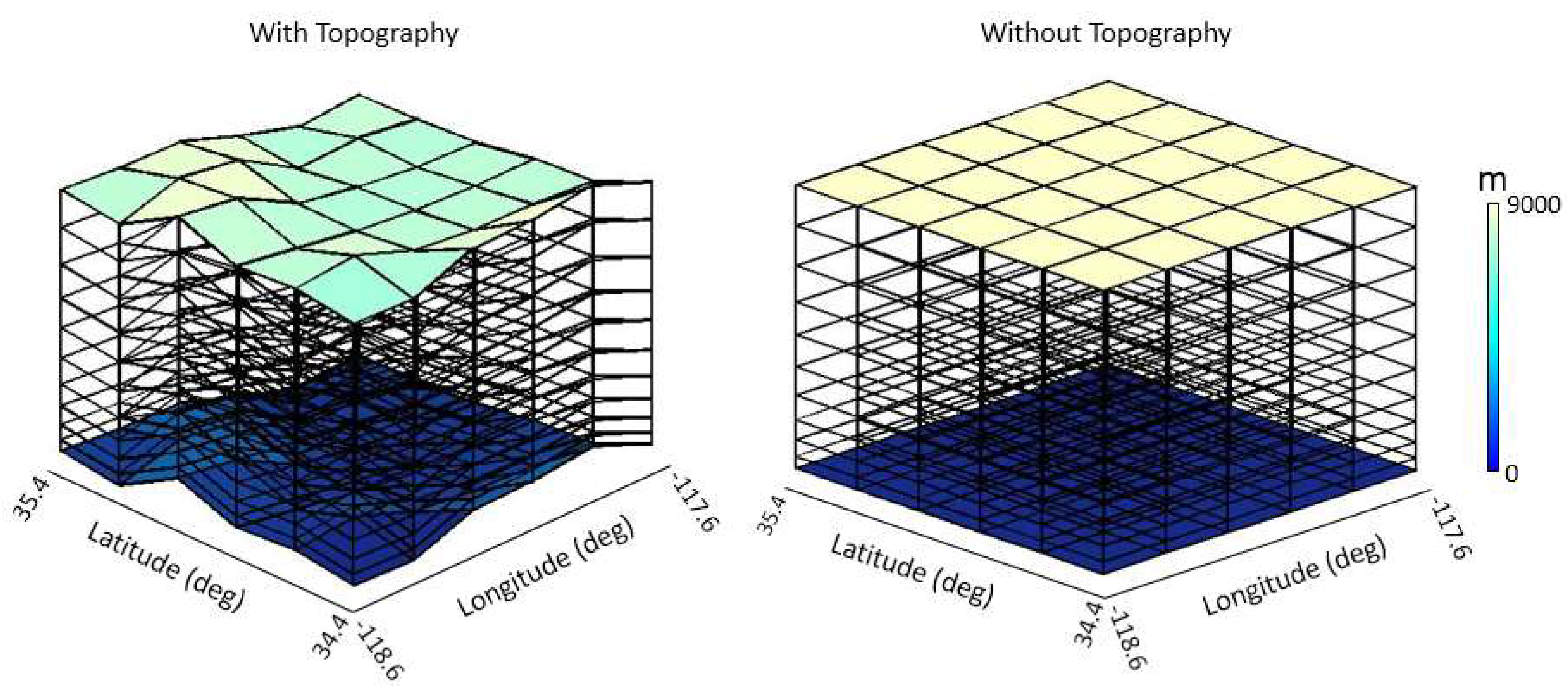
According to previous studies, the resolution of the tomography model should be selected based on the resolution matrix [11,27]. The model resolution matrix is one of the characteristics of the coefficient matrix and reflects the geometry and optimal resolution of the tomography model [11,27]. If any of the diagonal elements of the resolution matrix are trivial, the relevant parameters will be resolved poorly. The resolution matrix reflects the geometry and can be calculated during processing to access the optimal resolution for the tomography model. An optimal design of the tomography model results in a resolution matrix which is close to identity [11]. According to the resolution matrix, a horizontal resolution of 0.2 degrees was chosen for the basic tomography model (Figure 6). In this study, it was necessary to have a high resolution at the lower part of the tomography model in order to more accurately compare the variations. Therefore, the thickness of the vertical layers of the tomography model increases with the height (Figure 6). To analyze the effect of the topography, the processes were done in two different schemes. First, the tomography model was built without considering the topography of the study area. Second, the tomography model was built considering the topography of the area (Figure 6).

4.3. WRF Model Configuration

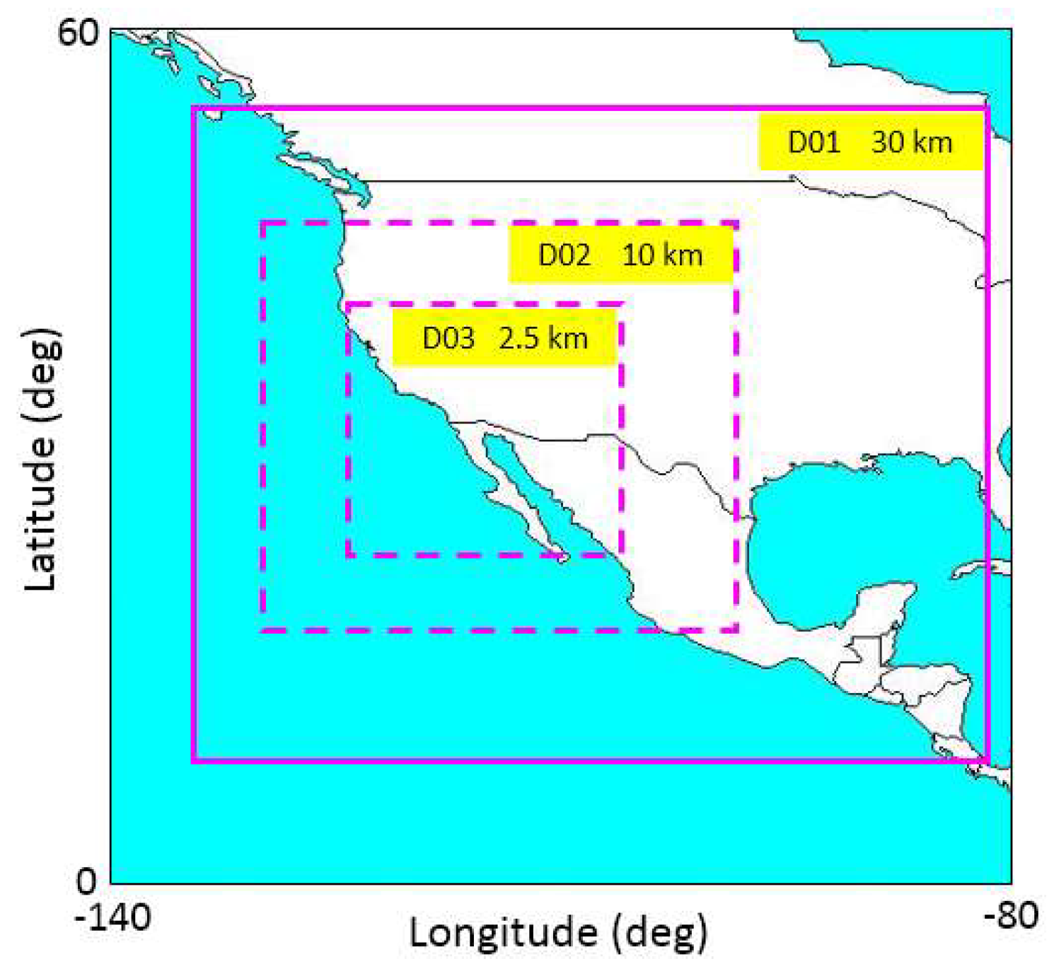
According to the above mentioned, the idea of this paper was to merge voxels based on the WRF model outputs. For this purpose, the WRF model should have been run at each epoch and before the tomography processing. In this paper, The WRF model version 3.8 was used with a set of parameters [28]. To run the WRF model, two nested domains (D02 and D03) were considered inside a parent outer domain (D01). The configuration of the domains and their resolution can be seen in Figure 7.
The list of physics schemes used in this model can be seen in Table 1. In the domain 03, the cumulus parameterization was turned off. In the larger domains, the Kain–Fritsch cumulus parameterization was used [29].
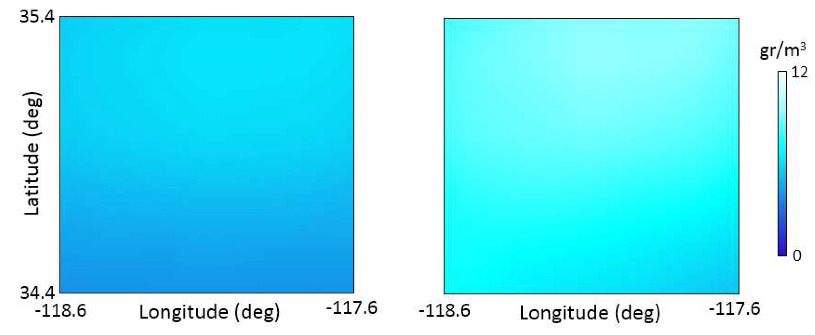
Figure 8 shows examples of the extracted WVD from the WRF model outputs.

5. Results and Discussion

In order to study the effect of using the WRF model and the topography of the area, the process was performed in four ways:
  • Scheme 1: using the topography and WRF model outputs.
  • Scheme 2: considering the topography of the area without using the WRF model.
  • Scheme 3: by applying the WRF model without using the topography.
  • Scheme 4: without the use of the topography and WRF model outputs.
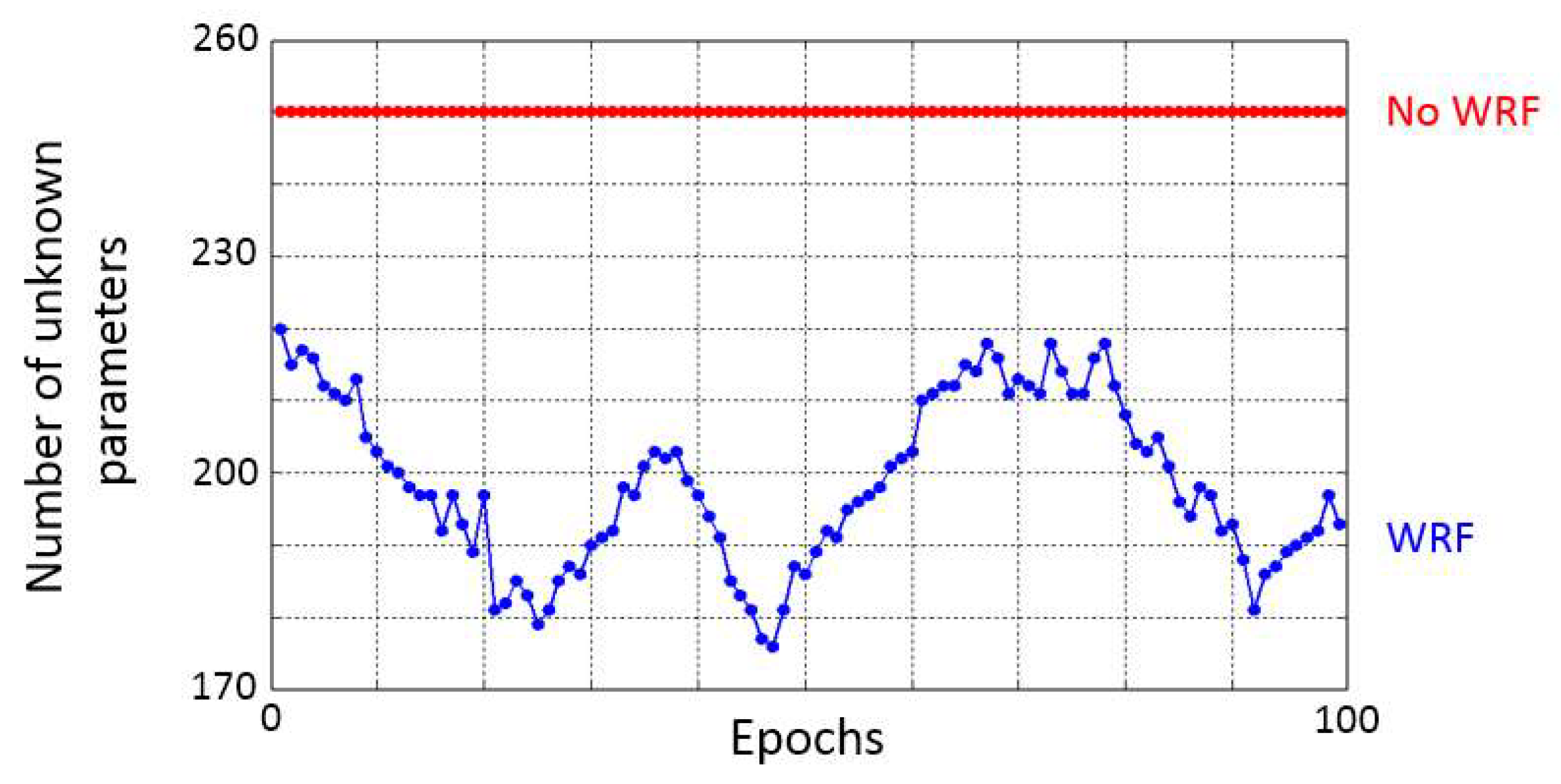
Figure 9 shows the role of using the WRF model to reduce the number of unknown parameters of the troposphere tomography problem.
Figure 10 shows an example of the estimated WVD field from four different schemes at a sample epoch.
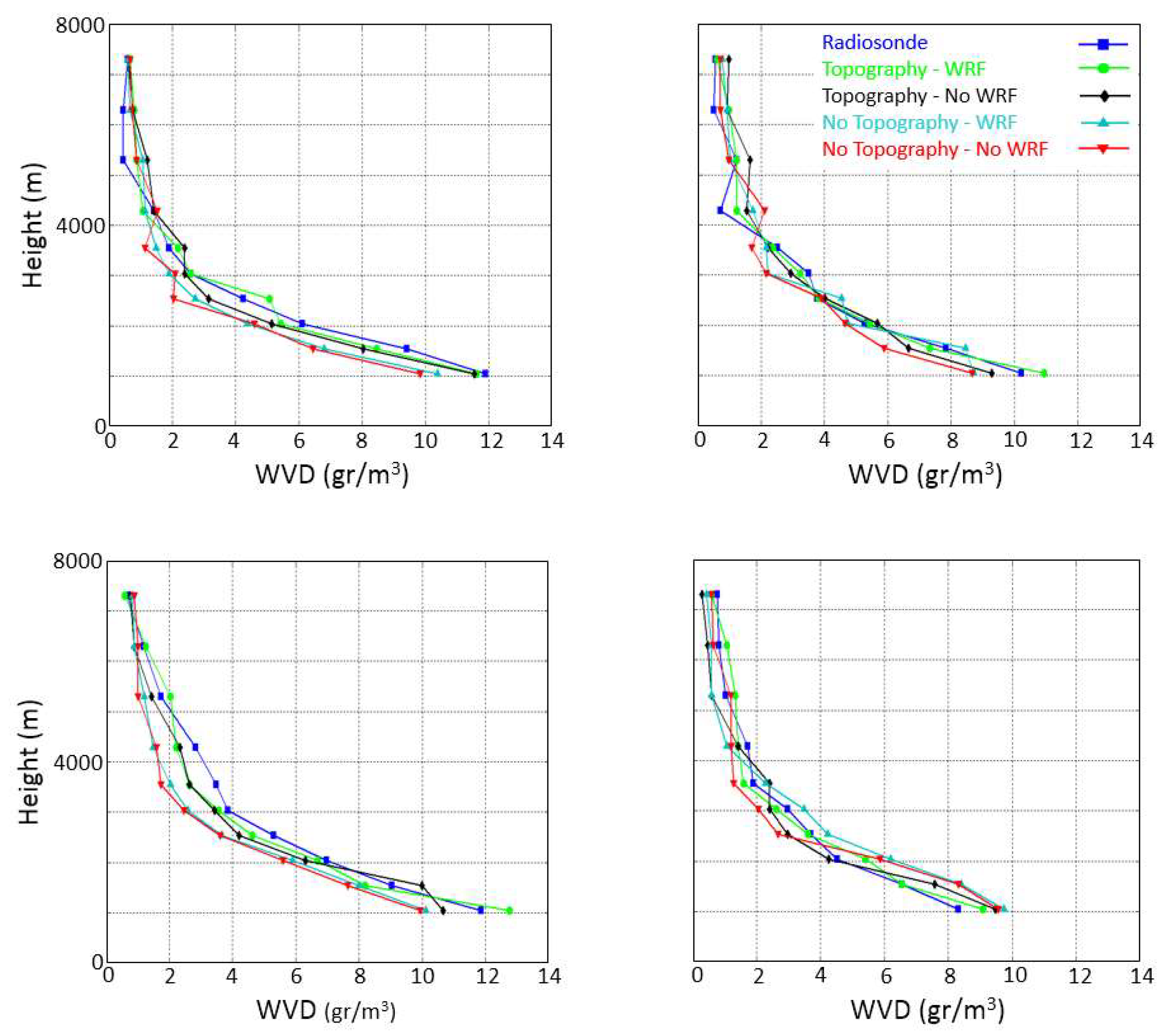
In order to validate the WVD from the four schemes, the results for the location of the radiosonde station wee compared with the radiosonde data for the experimental period. The examples of this comparison for four different epochs are visible in Figure 11 and Figure 12.
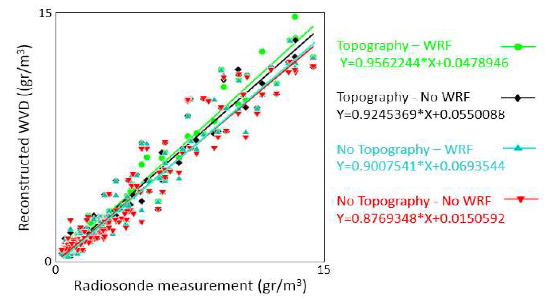
Table 2 shows the statistical parameters of the results obtained with the four troposphere tomography schemes and radiosonde measurements over the tested period. A scatter plot was used to better compare the obtained WVD (Figure 13).
The statistical results in Table 2 and the slope of the fitted lines in Figure 13 show that the water vapor obtained from the first scheme (Topography–WRF) is more consistent with the radiosonde observations. The worst results are related to the schemes that did not consider the topography of the area. This conclusion indicates the importance of using topography in the troposphere tomography problem. It can also be stated that using the WRF model outputs has a significant impact on improving the accuracy of the results. In order to compare these schemes more precisely, it is necessary to evaluate the results in another area of the tomography model. Therefore, the precise point positioning (PPP) technique was used for this purpose. Observations from one of the GPS stations in the tomography area were used for this validation.
First, the position time series of this station on the considered days was extracted from the Plate Boundary Observatory (PBO) GPS network (http://unavco.org).
The GPS tropospheric delay was computed using the obtained WVD from the four tomography schemes. Then, the code and phase observations of this GPS station were corrected using these four types of corrections. After this step, point positioning was performed using the PPP technique. Previous research has proved that the difference between tropospheric delay correction methods is more significant in wet weather conditions.
Therefore, the comparison was performed in two different weather conditions. The first category included days with an average humidity of more than 60% and the second group included days with an average humidity of less than 60%. Finally, the RMSE between the positions obtained using the four tomography schemes and the position obtained from the PBO GPS network was calculated (Figure 14, Table 3).
On days with less than 60% humidity, the difference between the RMSE computed from the first scheme and the other schemes is significant. The difference between the RMSE of the first two schemes in computing the up component is about 8 mm. This demonstrates the importance of using the WRF model outputs to improve the accuracy of the tomography results. The RMSEs obtained from the third and fourth schemes are close to each other. The importance of using the topography of the area is also clear in this comparison.
On days with more than 60% humidity, the difference between the RMSE of the two first schemes in the east, north and up components is about 8, 7 and 14 mm, respectively. Considering the accuracy of the PPP technique, these differences are significant and cannot be ignored. The highest and lowest differences between these two schemes are observed in the up and north components. Similar to the previous comparison, the role of topography in improving the accuracy is remarkable.
Based on all these validations, it can be concluded that the use of the WRF model outputs to eliminate redundant unknown parameters and to reduce the number of required constraints can significantly increase the accuracy of the troposphere tomography results. In addition, the topography of the area is one of the most important parameters that have a decisive role in the tomography results and should not be ignored.

6. Conclusions

In this article, an applicable idea based on the WRF model outputs was presented to optimize the troposphere tomography technique by merging voxels. In addition, the role and importance of using the topography of the area to improve the accuracy of the results was investigated. In conventional tomography, increasing the spatial resolution of the tomography model leads to an increase in the number of the unknown parameters of the problem and an increase in the required constraints. Based on the idea proposed in this paper, a high spatial resolution basic tomography model can be considered, but it is necessary to integrate the neighboring voxels with small differences in water vapor. This method can model water vapor with a higher accuracy wherever variations in this parameter are high. It also reduces the number of unknown parameters of the troposphere tomography problem. The WRF model outputs were used to merge the voxels before solving the tomography problem. The voxel integration criteria were determined based on a sensitivity analysis. In this paper, in addition to validating the ability of the new idea, the role and importance of using the topography of the area were also evaluated. The troposphere tomography was performed in four different schemes and then the obtained results were evaluated using radiosonde observations and the PPP technique. The four schemes were: Topography–WRF, Topography–No WRF, No Topography–WRF and No Topography–No WRF. Validation using the radiosonde data showed that the first scheme method had more power in reconstructing the WVD. Next, the PPP technique was used to evaluate the results in another area of the tomography model in different weather conditions. The results of this evaluation showed that considering the topography of the area and applying the WRF model outputs can lead to more accurate results in the troposphere tomography technique.

Author Contributions

Conceptualization, S.H.-A. and Y.A.; formal analysis, S.H.-A.; sensitivity analysis, H.M.; writing—original draft, S.H.-A; supervision—review and editing, Y.A., S.V. and W.R. All authors have read and agreed to the published version of the manuscript.

Funding

This research received no external funding.

Acknowledgments

Authors would like to appreciate the UNAVCO for the GPS observations and for providing high-accuracy station position time series. We are also grateful to the ECMWF for publishing ERA5 data.

Conflicts of Interest

The authors declare no conflict of interest.

References

  1. Merrikhpour, M.H.; Rahimzadegan, M. Improving the Algorithm of Extracting Regional Total Precipitable Water Vapor Over Land from MODIS Images. IEEE Trans. Geosci. Remote Sens. 2017, 55, 5889–5898. [Google Scholar] [CrossRef]
  2. Merrikhpour, M.H.; Rahimzadegan, M. Analysis of temporal and spatial variations of total precipitable water vapor in western Iran using radiosonde and MODIS measurements. J. Appl. Remote Sens. 2019, 13, 044508. [Google Scholar] [CrossRef]
  3. Flores, A.; Ruffini, G.; Rius, A. 4D tropospheric tomography using GPS slant wet delays. Ann. Geophys. Ger. 2000, 18, 223–234. [Google Scholar] [CrossRef]
  4. Hirahara, K. Local GPS tropospheric tomography. Earth Planets Space 2000, 52, 935–939. [Google Scholar] [CrossRef] [Green Version]
  5. Razin, M.R.G.; Voosoghi, B. Modeling of ionosphere time series using wavelet neural networks (case study: N-W of Iran). Adv. Space Res. 2016, 58, 74–83. [Google Scholar] [CrossRef]
  6. Rohm, W.; Bosy, J. Local tomography troposphere model over mountains area. Atmos. Res. 2009, 93, 777–783. [Google Scholar] [CrossRef]
  7. Rohm, W.; Zhang, K.; Bosy, J. Limited constraint, robust Kalman filtering for GNSS troposphere tomography. Atmos. Meas. Tech. 2014, 7, 1475–1486. [Google Scholar] [CrossRef] [Green Version]
  8. Yao, Y.; Zhao, Q. Maximally Using GPS Observation for Water Vapor Tomography. IEEE Trans. Geosci. Remote Sens. 2016, 54, 7185–7196. [Google Scholar] [CrossRef]
  9. Zhao, Q.; Yao, Y.; Cao, X.; Zhou, F.; Xia, P. An Optimal Tropospheric Tomography Method Based on the Multi-GNSS Observations. Remote Sens. 2018, 10, 234. [Google Scholar] [CrossRef] [Green Version]
  10. Zhao, Q.; Yao, Y.; Yao, W.; Xia, P. An optimal tropospheric tomography approach with the support of an auxiliary area. Ann. Geophys. 2018, 36, 1037–1046. [Google Scholar] [CrossRef] [Green Version]
  11. Haji-Aghajany, S.; Amerian, Y. Three dimensional ray tracing technique for tropospheric water vapor tomography using GPS measurements. J. Atmos. Solar Terr. Phys. 2017, 164, 81–88. [Google Scholar] [CrossRef]
  12. Haji-Aghajany, S.; Amerian, Y. Hybrid Regularized GPS Tropospheric Sensing Using 3-D Ray Tracing Technique. IEEE Geosci. Remote Sens. Lett. 2018, 15, 1475–1479. [Google Scholar] [CrossRef]
  13. Heublein, M.; AlShawaf, F.; Erdnüß, B.; Zhu, X.X.; Hinz, S. Compressive sensing reconstruction of 3D wet refractivity based on GNSS and InSAR observations. J. Geod. 2018, 93, 197–217. [Google Scholar] [CrossRef] [Green Version]
  14. Zhao, Q.; Yao, Y. An improved troposphere tomographic approach considering the signals coming from the side face of the tomographic area. Ann. Geophys. 2017, 35, 87–95. [Google Scholar] [CrossRef] [Green Version]
  15. Zhao, Q.; Zhang, K.; Yao, Y.; Li, X. A new troposphere tomography algorithm with a truncation factor model (TFM) for GNSS networks. GPS Solut. 2019, 23, 64. [Google Scholar] [CrossRef]
  16. Zhao, Q.; Yao, W.; Yao, Y.; Li, X. An improved GNSS tropospheric tomography method with the GPT2w model. GPS Solut. 2020, 24, 1–13. [Google Scholar] [CrossRef]
  17. Brenot, H.; Rohm, W.; Kačmařík, M.; Möller, G.; Sá, A.; Tondaś, D.; Rapant, L.; Biondi, R.; Manning, T.; Champollion, C. Cross-Comparison and Methodological Improvement in GPS Tomography. Remote Sens. 2019, 12, 30. [Google Scholar] [CrossRef] [Green Version]
  18. Bevis, M.; Businger, S.; Herring, T.; Rocken, C.; Anthes, R.A.; Ware, R.H. GPS meteorology: Remote sensing of atmospheric water vapor using the global positioning system. J. Geophys. Res. Space Phys. 1992, 97, 15787. [Google Scholar] [CrossRef]
  19. Saastamoinen, J. Contributions to the theory of atmospheric refraction. J. Geod. 1973, 107, 13–34. [Google Scholar] [CrossRef]
  20. Chen, B.; LiuiD, Z. Voxel-optimized regional water vapor tomography and comparison with radiosonde and numerical weather model. J. Geod. 2014, 88, 691–703. [Google Scholar] [CrossRef]
  21. Rodgers, J.L.; Nicewander, W.A. Thirteen Ways to Look at the Correlation Coefficient. Am. Stat. 1988, 42, 59. [Google Scholar] [CrossRef]
  22. Haji-Aghajany, S.; Voosoghi, B.; Yazdian, A. Estimation of north Tabriz fault parameters using neural networks and 3D tropospherically corrected surface displacement field. Geomat. Nat. Hazards Risk 2017, 8, 918–932. [Google Scholar] [CrossRef] [Green Version]
  23. Haji-Aghajany, S.; Voosoghi, B.; Amerian, Y. Estimating the slip rate on the north Tabriz fault (Iran) from InSAR measurements with tropospheric correction using 3D ray tracing technique. Adv. Space Res. 2019, 64, 2199–2208. [Google Scholar] [CrossRef]
  24. Hersbach, H.; Dee, D. ERA5 Reanalysis is in Production; ECMWF Newsletter 147; ECMWF: Reading, UK, 2016. [Google Scholar]
  25. Michalakes, J.; Dudhia, J.; Gill, D.; Henderson, T.; Klemp, J.; Skamarock, W.; Wang, W. The Weather Reseach and Forecast Model: Software Architecture and Performance. In Proceedings of the 11th ECMWF Workshop on the Use of High Performance Computing in Meteorology, 25−29 October 2004; Mozdzynski, G., Ed.; ECMWF: Reading, UK, 2004. [Google Scholar]
  26. Dach, R.; Lutz, S.; Walser, P.; Fridez, P. (Eds.) Bernese GNSS Software Version 5.2. User Manual, Astronomical Institute; Open Publishing; University of Bern: Bern, Switzerland, 2015; ISBN 978-3-906813-05-9. [Google Scholar] [CrossRef]
  27. Bender, M.; Stosius, R.; Zus, F. GNSS water vapour tomography – Expected improvements by combining GPS, GLONASS and Galileo observations. Adv. Space Res. 2011, 47, 886–897. [Google Scholar] [CrossRef]
  28. Skamarock, W.C.; Klemp, J.B.; Dudhia, J.; Gill, D.O.; Barker, M.; Duda, K.G.; Huang, Y.; Wang, W.; Powers, J.G. A Description of the Advanced Research WRF; Version 3; National Center for Atmospheric Research Boulder Co Mesoscale and Microscale Meteorology Div: Boulder, CO, USA, 2008; pp. 1–113. [Google Scholar]
  29. Kain, J.S. The Kain–Fritsch Convective Parameterization: An Update. J. Appl. Meteorol. 2004, 43, 170–181. [Google Scholar] [CrossRef] [Green Version]
  30. Hong, S.-Y.; Lim, J.-O.J. The WRF single-moment 6-class microphysics scheme (WSM6). J. Korean Meteorol. Soc. 2006, 42, 129–151. [Google Scholar]
  31. Iacono, M.J.; Delamere, J.S.; Mlawer, E.J.; Shephard, M.W.; Clough, S.A.; Collins, W. Radiative forcing by long-lived greenhouse gases: Calculations with the AER radiative transfer models. J. Geophys. Res. Space Phys. 2008, 113, 13103. [Google Scholar] [CrossRef]
  32. Chou, M.-D.; Suarez, M.J. A Solar Radiation Parameterization for Atmospheric Studies. In Technical Report Series on Global Modeling and Data Assimilation; NASA/TM-1999-104606; NASA: Washington, DC, USA, 1999; Volume 15. [Google Scholar]
  33. Niu, G.-Y.; Yang, Z.; Mitchell, K.E.; Chen, F.; Ek, M.B.; Barlage, M.; Kumar, A.; Manning, K.; Niyogi, D.; Rosero, E.; et al. The community Noah land surface model with multiparameterization options (Noah-MP): 1. Model description and evaluation with local-scale measurements. J. Geophys. Res. Space Phys. 2011, 116. [Google Scholar] [CrossRef] [Green Version]
  34. Hong, S.Y.; Noh, Y.; Dudhia, J. A new vertical di_usion package with an explicit treatment of entrainment processes. Mon. Weather Rev. 2006, 134, 2318–2341. [Google Scholar] [CrossRef] [Green Version]
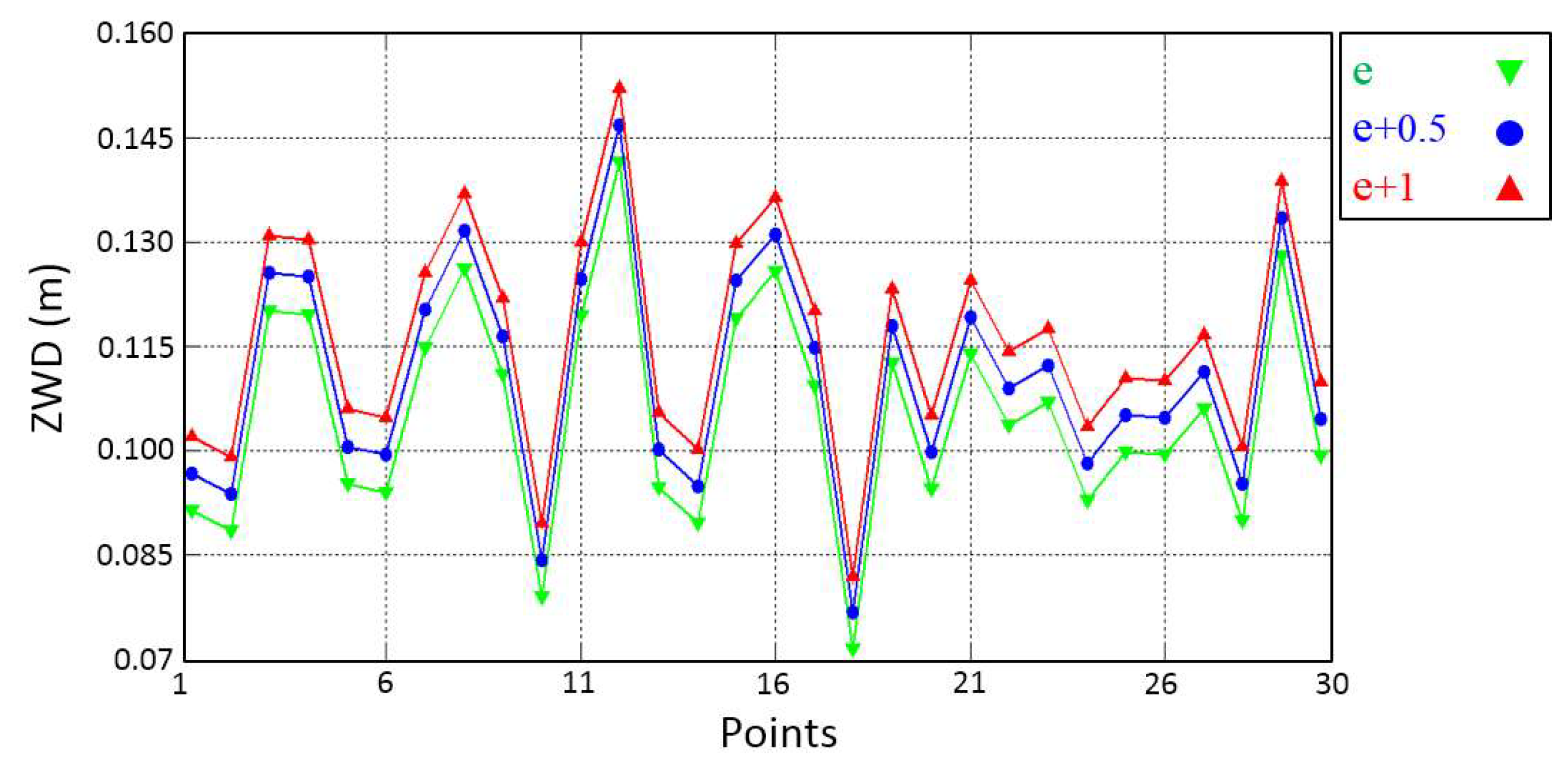
Figure 1. An example of the sensitivity analysis of the zenith wet delay (ZWD) to changes in water vapor pressure e [hPa]. The green line shows the computed ZWD using the actual e. The blue and red lines indicate the computed ZWD using changed e in all layers.
Remotesensing 12 01442 g001
Figure 2. The effect of on the estimated position (blue lines) in different modes and for different ZWD offsets. The orange lines show the position dilution of precision (PDOP)/number of satellites.
Remotesensing 12 01442 g002
Figure 3. The process of performing the merging voxels based on the Weather Research and Forecasting (WRF) model.
Remotesensing 12 01442 g003
Figure 4. Geographical location of the study area.
Remotesensing 12 01442 g004
Figure 5. Topography of the study area and the distribution of the Global Positioning System (GPS) stations. The blue square represents the radiosonde station and the red triangle shows the position of the station used to evaluate the results.
Remotesensing 12 01442 g005
Figure 6. Considered basic tomography models for this study.
Remotesensing 12 01442 g006
Figure 7. Configuration of the domains around the study area.
Remotesensing 12 01442 g007
Figure 8. Obtained water vapor density (WVD) from the WRF model at a pressure level of 900 mb at two sample epochs.
Remotesensing 12 01442 g008
Figure 9. Comparison of the number of unknown parameters at different epochs.
Remotesensing 12 01442 g009
Figure 10. An example of the obtained WVD field.
Remotesensing 12 01442 g010
Figure 11. Two examples of comparison between the obtained WVD and radiosonde observations.
Remotesensing 12 01442 g011
Figure 12. Two examples of the absolute value of the difference between the radiosonde observations and the obtained results.
Remotesensing 12 01442 g012
Figure 13. Scatter plot between the reconstructed WVD and radiosonde measurements.
Remotesensing 12 01442 g013
Figure 14. Positioning RMSE in different weather conditions.
Remotesensing 12 01442 g014
Table 1. The physics schemes used in the WRF configuration.
CategorySchemeReference
Longwave radiationWRF single-moment 6 class[30]
Shortwave radiationRapid Radiative Transfer Model[31]
Land surfaceGoddard[32]
Planetary boundary layerNoah-MP (multi physics)[33]
microphysicsYonsei University[34]
Table 2. Statistical comparison between the obtained WVD and radiosonde data.
SchemeRMSE
(gr/m3)
Bias
(gr/m3)
Min-Diff
(gr/m3)
Max-Diff
(gr/m3)
PCC
Topography–WRF0.6120.0090.0610.9610.981
Topography–No WRF0.9710.0140.0821.3780.972
No Topography–WRF1.2340.0210.1232.6180.944
No Topography–No WRF1.4150.0240.1372.960.931
Table 3. Comparison of the obtained RMSE.
RMSE in Days with Humidity Less than 60% (mm)RMSE in Days with Humidity More than 60% (mm)
EastNorthUpEastNorthUp
Topography–WRF12.9210.1314.0120.4418.7717.11
Topography–No WRF19.8116.6321.1927.9125.5330.67
No Topography–WRF23.8428.1430.1536.4529.4838.65
No Topography–No WRF29.0521.5931.8737.8629.2337.14