Structure-From-Motion Photogrammetry of Antarctic Historical Aerial Photographs in Conjunction with Ground Control Derived from Satellite Data


Abstract
:
1. Introduction
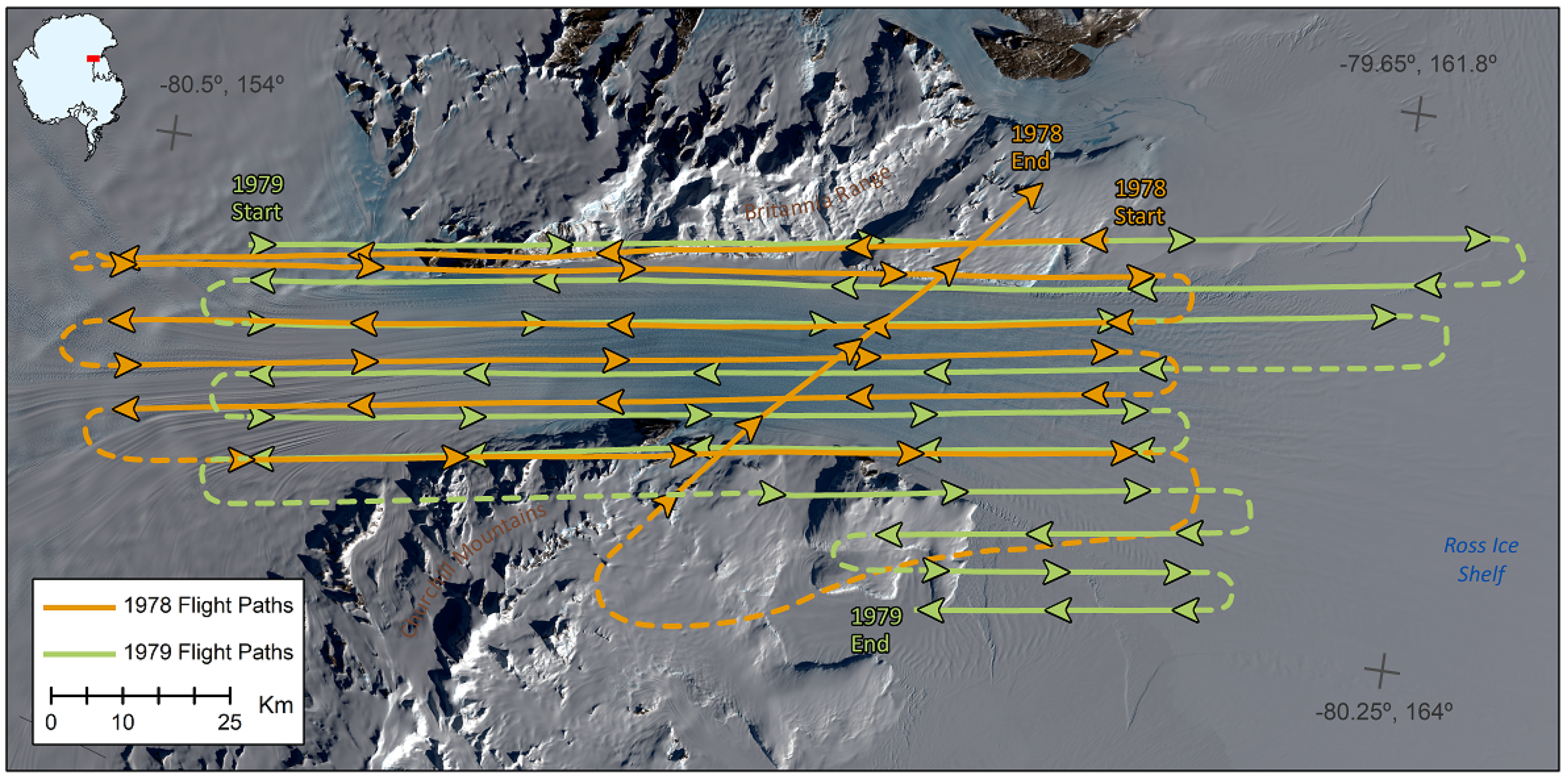
2. Study Site
3. Materials
3.1. Aerial Photography
3.1.1. Imagery
3.1.2. Original Study
3.2. High-Resolution DEM
3.3. Rock Mask
3.4. GPS Data
3.5. Ice Thickness
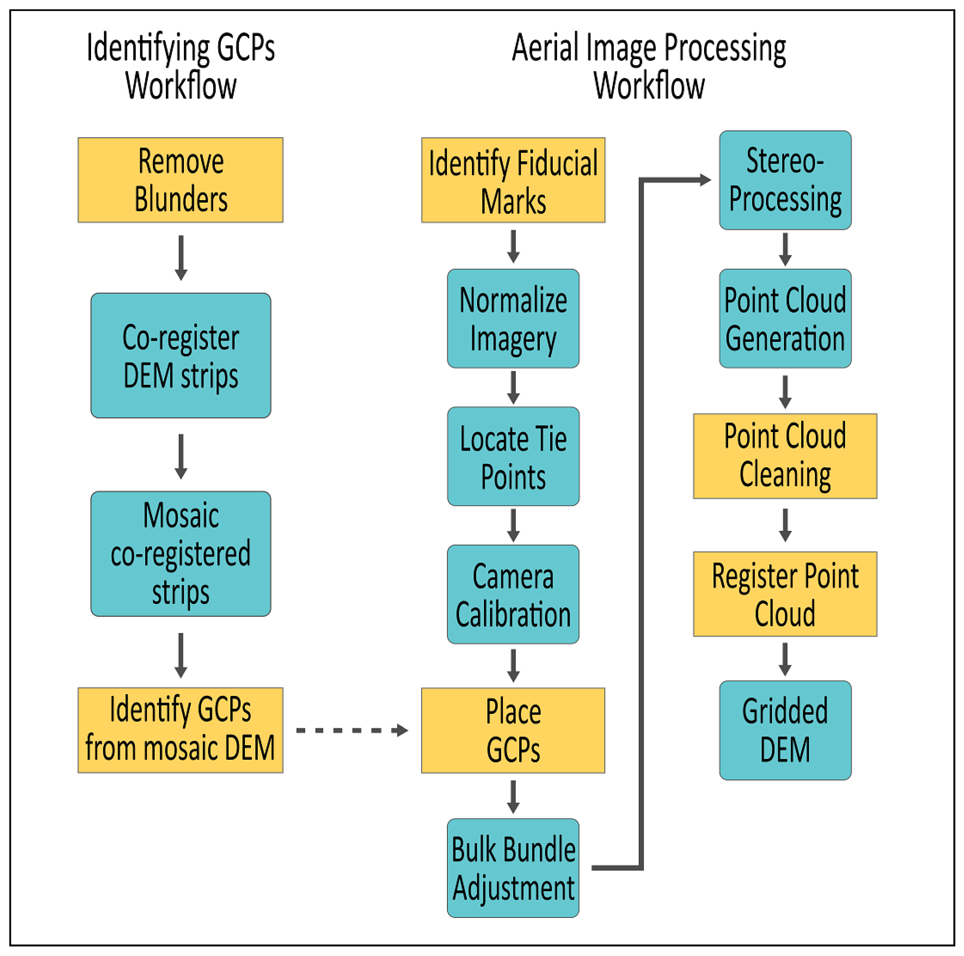
4. Methods
4.1. Ground Control Points
4.1.1. Blunder/Cloud/Shadow Masking
4.1.2. Coregistering/Mosaicking
4.1.3. Identifying GCPs
4.2. Elevation Processing
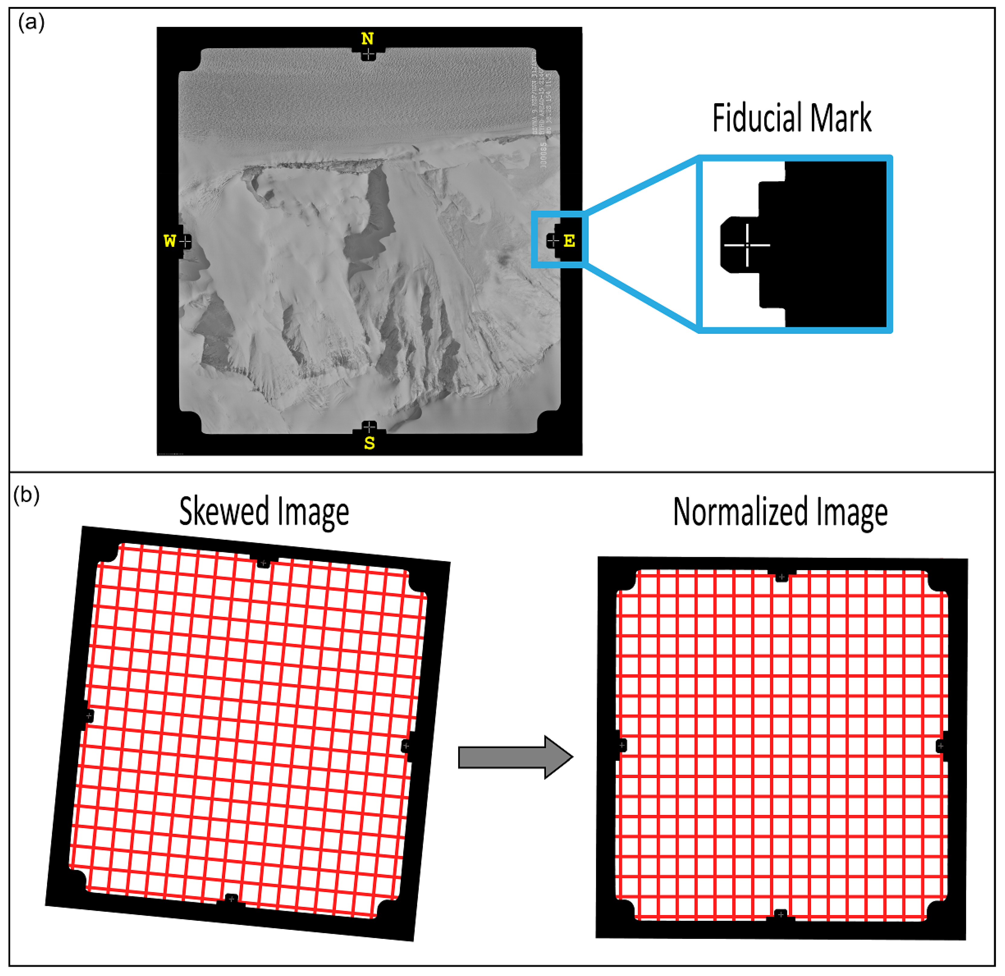
4.2.1. Interior Orientation
4.2.2. Relative Orientation
4.2.3. Absolute Orientation
4.2.4. DEM
4.2.5. DEM Registration
4.3. Velocity
4.4. Data Validation
4.4.1. Elevation Comparisons
4.4.2. Velocity Comparisons
4.4.3. Grounding Zone
4.4.4. Basal Evolution
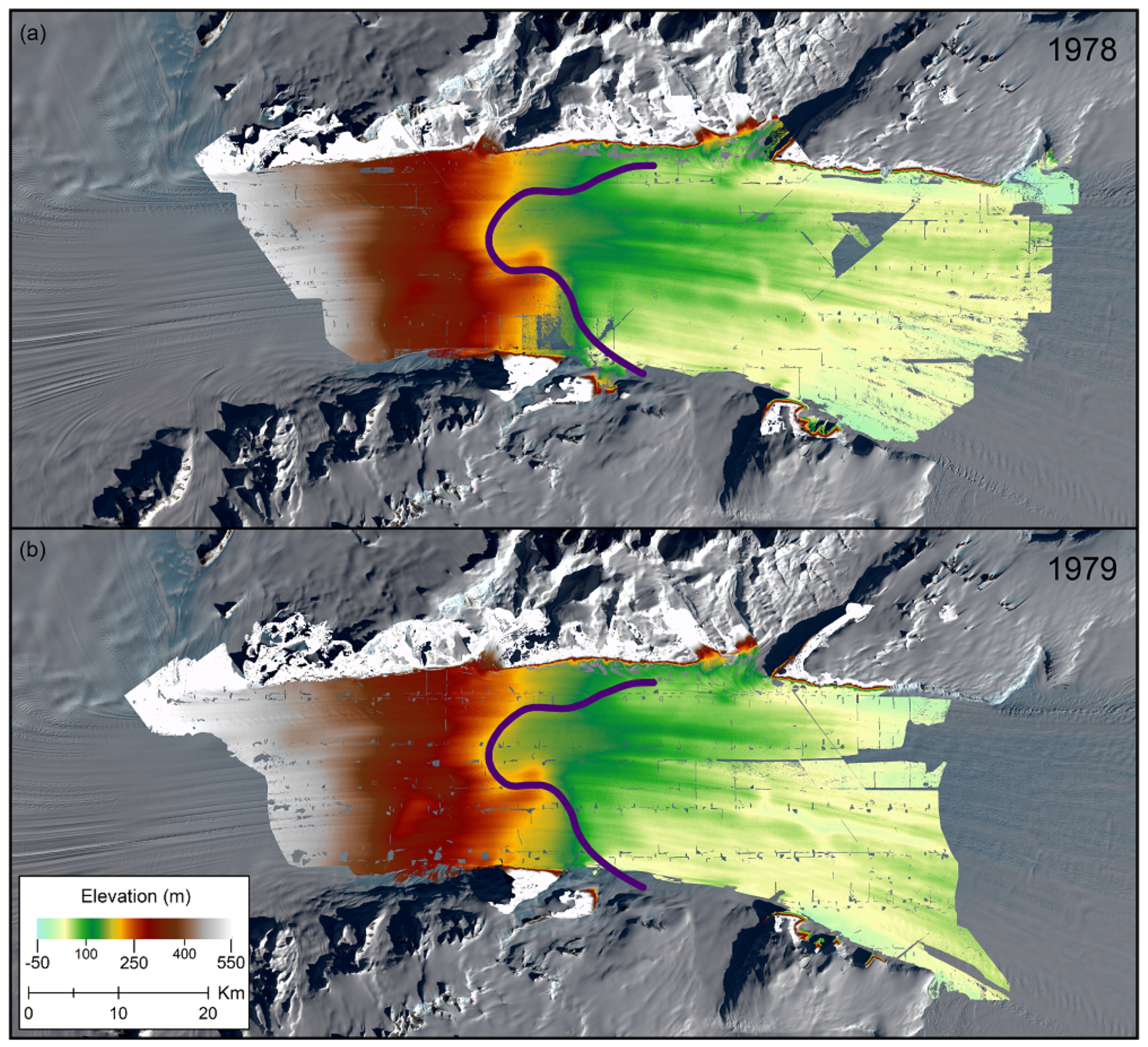
5. Results and Discussion
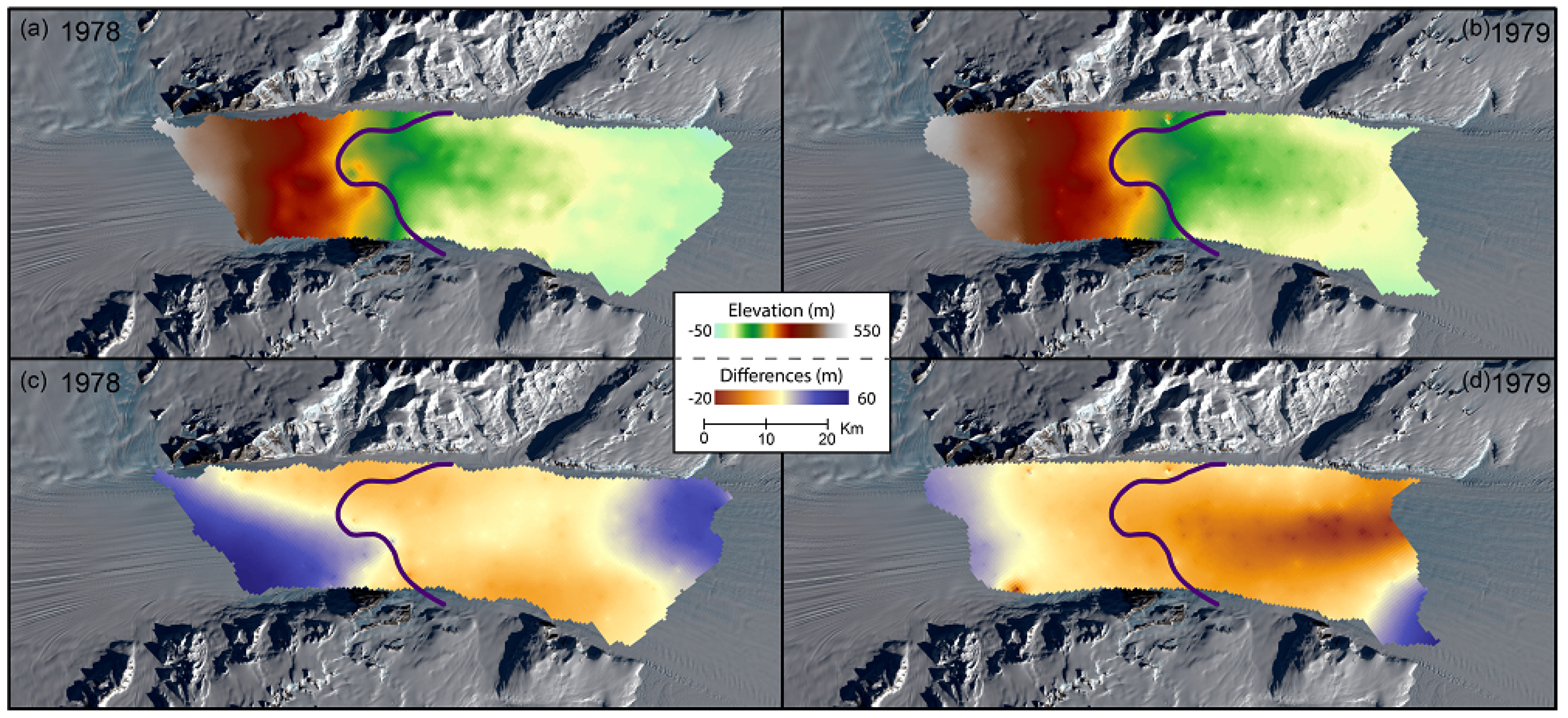
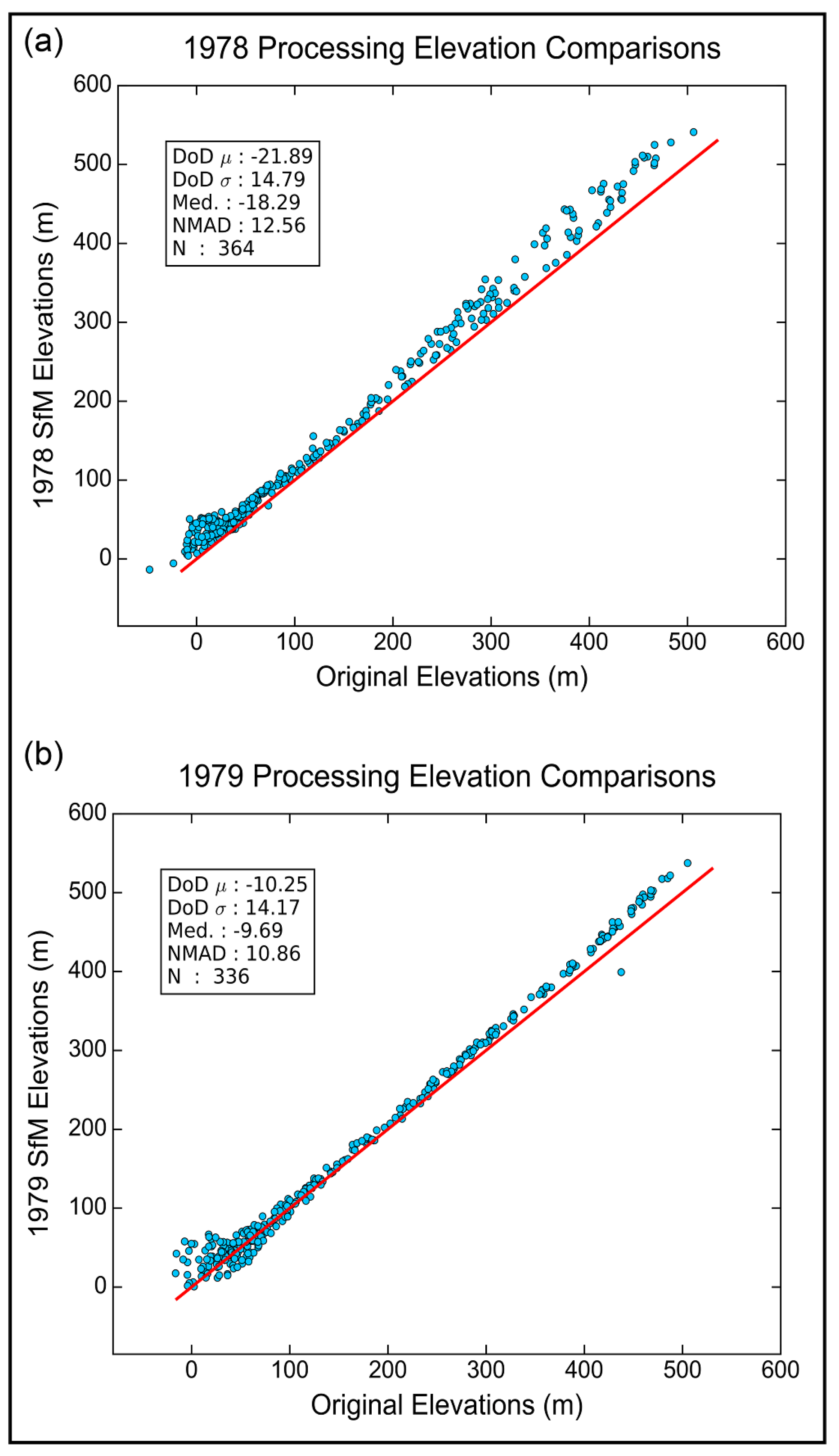
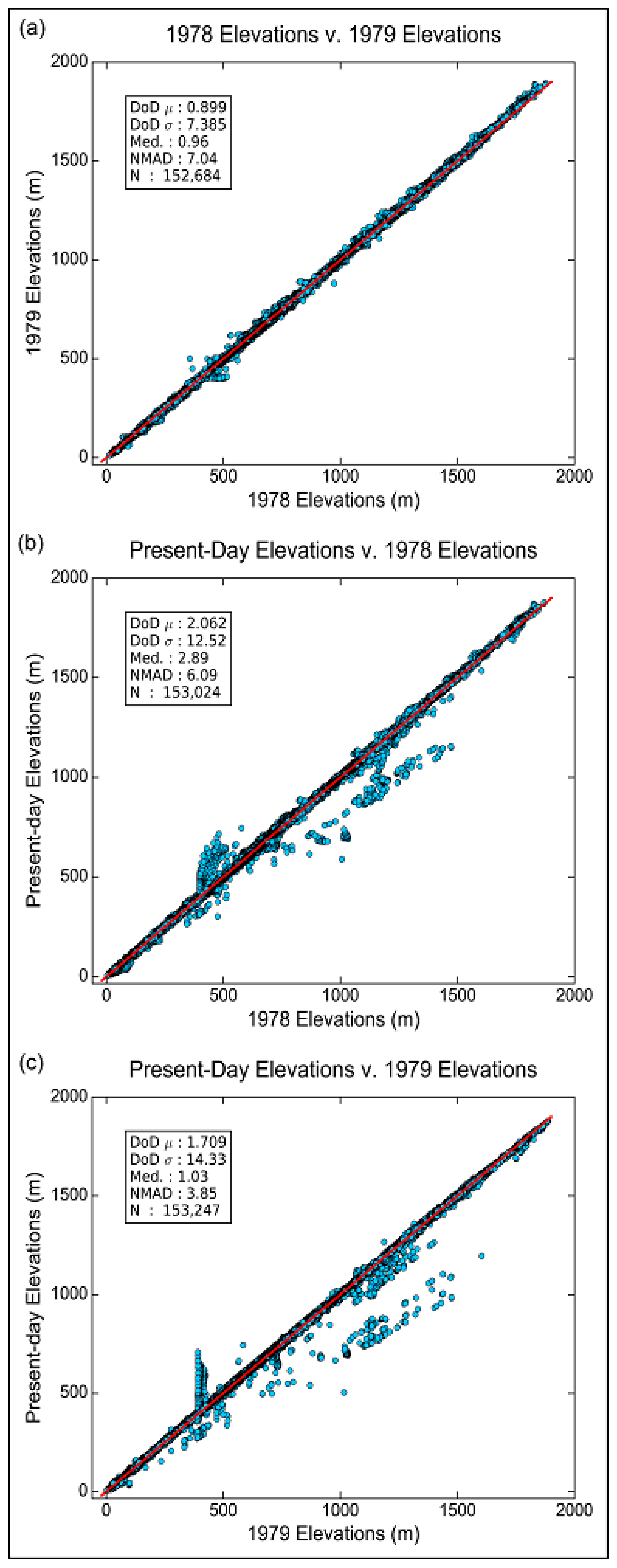
5.1. DEM Products
Estimated Accuracy
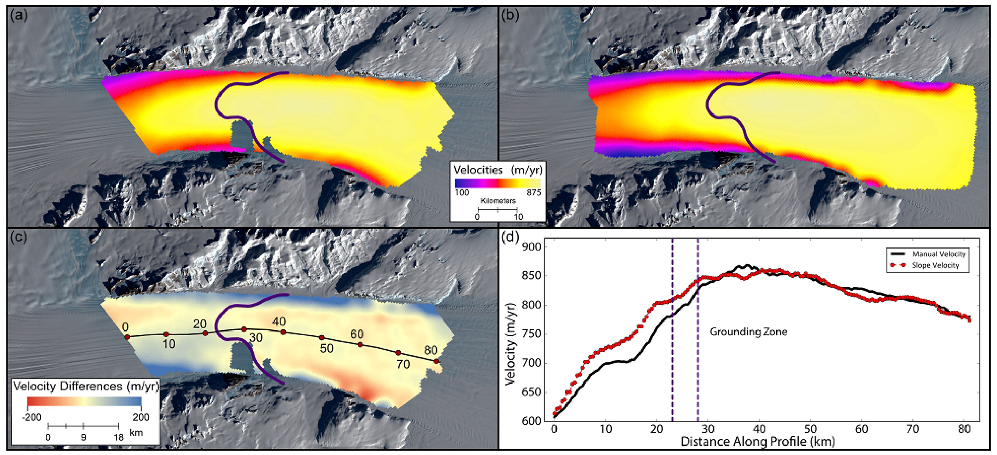
5.2. Velocity
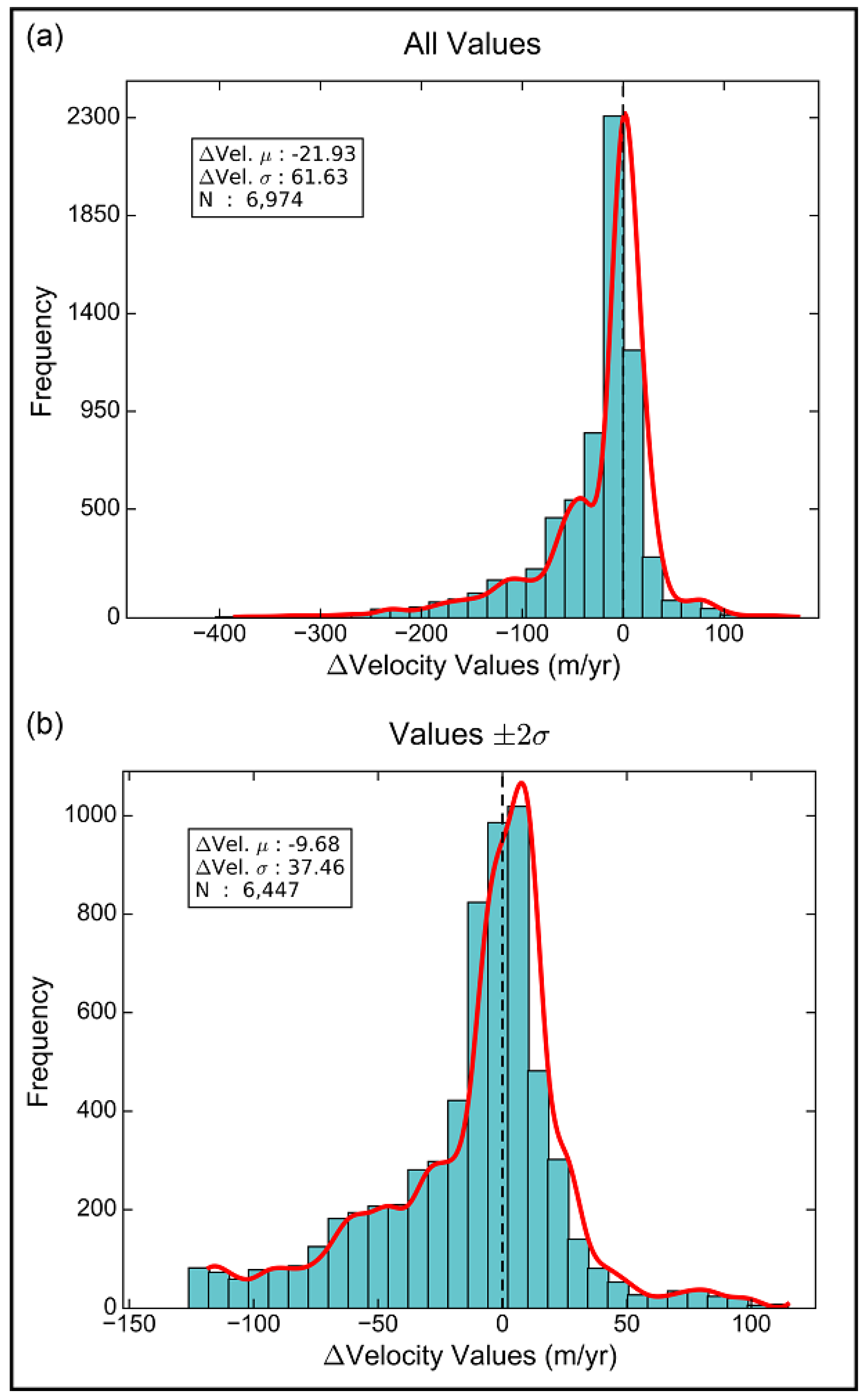
Velocity Differences
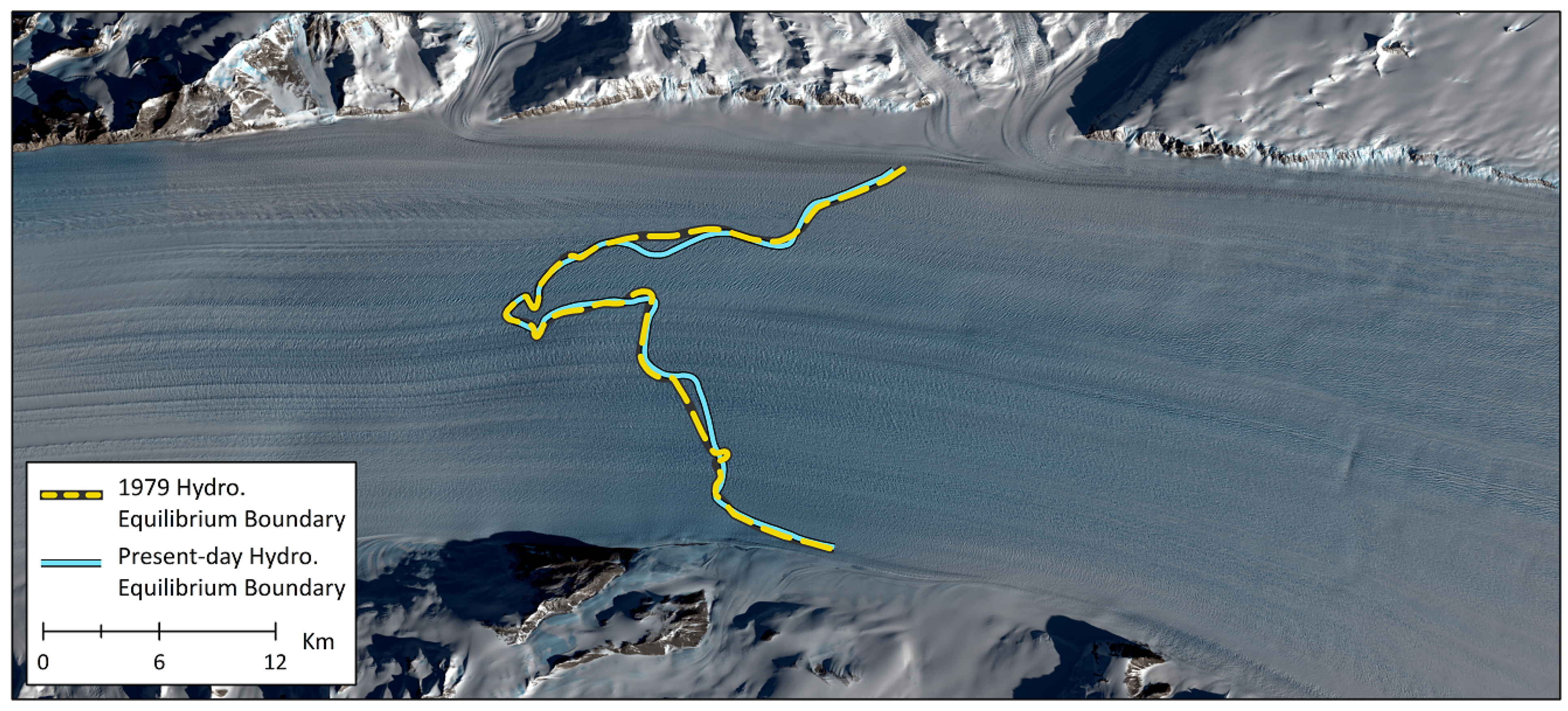
5.3. Grounding Zone
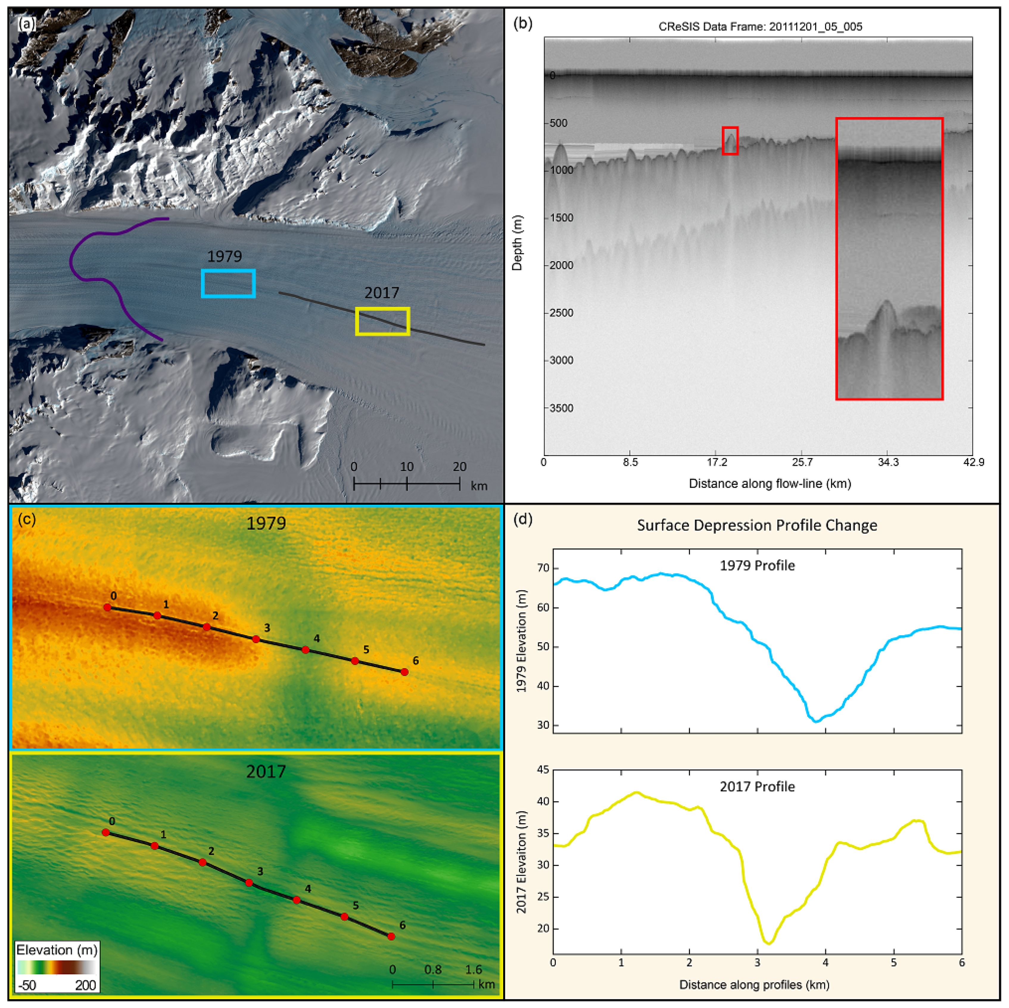
5.4. Basal Evolution
6. Conclusions
Supplementary Materials
Author Contributions
Funding
Acknowledgments
Conflicts of Interest
References
- Anisimov, O.A.; Vaughan, D.G.; Callaghan, T.V.; Furgal, C.; Marchant, H.; Prowse, T.D.; Vilhjálmsson, H.; Walsh, J. (Eds.) Polar regions (Arctic and Antarctic). Climate Change 2007: Impacts, Adaptation and Vulnerability. Contribution of Working Group II to the Fourth Assessment Report of the Intergovernmental Panel on Climate Change; IPCC, Cambridge University Press: Cambridge, UK, 2007. [Google Scholar]
- Vaughan, D.G.; Comiso, J.C.; Allison, I.; Carrasco, J.; Kaser, G.; Kwok, R.; Mote, P.; Murray, T.; Paul, F.; Ren, J.; et al. Observations: Cryosphere. In Climate Change 2013: The Physical Science Basis. Contribution of Working Group I to the Fifth Assessment Report of the Intergovernmental Panel on Climate Change; Stocker, T., Qin, D., Plattner, G.K., Tignor, G.K., Allen, S.K., Boschung, J., Nauels, A., Xia, Y., Bex, V., Midgley, P.M., Eds.; Intergovernmental Panel on Climate Change 2013; Cambridge University Press: Cambridge, UK; New York, NY, USA, 2013; pp. 317–382. [Google Scholar]
- Meredith, M.; Sommerkorn, M.; Cassotta, S.; Derksen, C.; Ekaykin, A.; Hollowed, A.; Kofinas, G.; Mackintosh, A.; Melbourne-Thomas, J.; Muelbert, M.; et al. Polar Regions. IPCC Special Report on the Ocean and Cryosphere in a Changing Climate. 2019. Available online: https://www.ipcc.ch/srocc/cite-report/ (accessed on 16 December 2020).
- Joerg, W.L.G. Demonstration of the Peninsularity of Palmer Land, Antarctica, Through Ellsworth’s Flight of 1935. Proc. Am. Philos. Soc. 1940, 82, 821–832. [Google Scholar]
- Richter, H. Mapping by aerial Photography in Antarctica. Int. Hydrogr. Rev. 1943, 20, 32–34. [Google Scholar]
- Cook, A.J.; Fox, A.J.; Vaughan, D.G.; Ferrigno, J.G. Retreating glacier fronts on the Antarctic Peninsula over the past half-century. Science 2005, 308, 541–544. [Google Scholar] [CrossRef] [Green Version]
- Fox, A.J.; Cziferszky, A. Unlocking the time capsule of historic aerial photography to measure changes in Antarctic Peninsula glaciers. Photogramm. Rec. 2008, 23, 51–68. [Google Scholar] [CrossRef] [Green Version]
- Guzzetti, F.; Mondini, A.C.; Cardinali, M.; Fiorucci, F.; Santangelo, M.; Chang, K.T. Landslide inventory maps: New tools for an old problem. Earth-Sci. Rev. 2012, 112, 42–66. [Google Scholar] [CrossRef] [Green Version]
- Bjørk, A.A.; Kjær, K.H.; Korsgaard, N.J.; Khan, S.A.; Kjeldsen, K.K.; Andresen, C.S.; Box, J.E.; Larsen, N.K.; Funder, S. An aerial view of 80 years of climate-related glacier fluctuations in southeast Greenland. Nat. Geosci. 2012, 5, 427–432. [Google Scholar] [CrossRef] [Green Version]
- Schiefer, E.; Gilbert, R. Reconstructing morphometric change in a proglacial landscape using historical aerial photography and automated DEM generation. Geomorphology 2007, 88, 167–178. [Google Scholar] [CrossRef]
- Girod, L.; Nielsen, N.I.; Couderette, F.; Nuth, C.; Kääb, A. Precise DEM extraction from Svalbard using 1936 high oblique imagery. Geoscientific Instrumentation. Methods Data Syst. 2018, 7, 277–288. [Google Scholar]
- Nielsen, N.I. Recovering Data with Digital Photogrammetry and Image Analysis Using Open Source Software. Master’s Thesis, University of Oslo, Oslo, Norway, 2017. [Google Scholar]
- Hughes, T.J.; Fastook, J.L. Byrd Glacier: 1978–1979 field results. Antarct. J. US 1981, 16, 86–89. [Google Scholar]
- Brecher, H.H. Photographic determination of surface velocities and elevations on Byrd Glacier. Antarct. J. 1982, 17, 79–81. [Google Scholar]
- Urbini, S.; Bianchi-Fasani, G.; Mazzanti, P.; Rocca, A.; Vittuari, L.; Zanutta, A.; Girelli, V.A.; Serafini, M.; Zirizzotti, A.; Frezzotti, M. Multi-Temporal Investigation of the Boulder Clay Glacier and Northern Foothills (Victoria Land, Antarctica) by Integrated Surveying Techniques. Remote Sens. 2019, 11, 1501. [Google Scholar] [CrossRef] [Green Version]
- Byrd, R.E.; Saunders, H.E. The Flight to Marie Byrd Land: With a Description of the Map. Geogr. Rev. 1933, 23, 177–209. [Google Scholar] [CrossRef]
- Joerg, W.L.G. The cartographical results of Ellsworth’s trans-Antarctic flight of 1935. Geogr. Rev. 1937, 27, 430–444. [Google Scholar] [CrossRef]
- USGS. USGS EROS Archive-Aerial Photography-Antarctic Single Frame Records. 2018. Available online: https://www.usgs.gov/centers/eros/science/usgs-eros-archive-aerial-photography-antarctic-single-frame-records?qt-science_center_objects=0#qt-science_center_objects (accessed on 16 December 2020).
- Rignot, E.; Mouginot, J.; Scheuchl, B.; van den Broeke, M.; van Wessem, M.J.; Morlighem, M. Four decades of Antarctic Ice Sheet mass balance from 1979–2017. Proc. Natl. Acad. Sci. USA 2019, 116, 1095–1103. [Google Scholar] [CrossRef] [Green Version]
- Stearns, L.A. Outlet Glacier Dynamics in East Greenland and East Antarctica. Ph.D. Dissertation, University of Maine, Orono, ME, USA, 2007. [Google Scholar]
- Taymen, W. Report of Calibration of Aerial Mapping Camera: Wild Heerbrugg RC8; Technical Report RT-R/399; United States Department of the Interior: Reston, VA, USA, 1978. [Google Scholar]
- Howat, I.M.; Porter, C.; Smith, B.E.; Noh, M.J.; Morin, P. The reference elevation model of Antarctica. Cryosphere 2019, 13, 665–674. [Google Scholar] [CrossRef] [Green Version]
- Noh, M.J.; Howat, I.M. Automated stereo-photogrammetric DEM generation at high latitudes: Surface Extraction with TIN-based Search-space Minimization (SETSM) validation and demonstration over glaciated regions. GIScience Remote Sens. 2015, 52, 198–217. [Google Scholar] [CrossRef]
- DigitalGlobe. Geolocation Accuracy of WorldView Products; White Paper; DigtialGlobe: Westminster, CO, USA, 2014. [Google Scholar]
- Noh, M.J.; Howat, I.M. The surface extraction from TIN based search-space minimization (SETSM) algorithm. ISPRS J. Photogramm. Remote Sens. 2017, 129, 55–76. [Google Scholar] [CrossRef]
- Glennie, C. Arctic high-resolution elevation models: Accuracy in sloped and vegetated terrain. J. Surv. Eng. 2018, 144, 06017003. [Google Scholar] [CrossRef]
- Nuth, C.; Kääb, A. Co-registration and bias corrections of satellite elevation data sets for quantifying glacier thickness change. Cryosphere 2011, 5, 271–290. [Google Scholar] [CrossRef] [Green Version]
- Paul, F.; Bolch, T.; Briggs, K.; Kääb, A.; McMillan, M.; McNabb, R.; Nagler, T.; Nuth, C.; Rastner, P.; Strozzi, T.; et al. Error sources and guidelines for quality assessment of glacier area, elevation change, and velocity products derived from satellite data in the Glaciers_cci project. Remote Sens. Environ. 2017, 203, 256–275. [Google Scholar] [CrossRef] [Green Version]
- Burton-Johnson, A.; Black, M.; Fretwell, P.; Kaluza-Gilbert, J. An automated methodology for differentiating rock from snow, clouds and sea in Antarctica from Landsat 8 imagery: A new rock outcrop map and area estimation for the entire Antarctic continent. Cryosphere 2016, 10, 1665–1677. [Google Scholar] [CrossRef] [Green Version]
- Lichten, S.M.; Border, J.S. Strategies for high-precision Global Positioning System orbit determination. J. Geophys. Res. Solid Earth 1987, 92, 12751–12762. [Google Scholar] [CrossRef]
- Elósegui, P.; Davis, J.L.; Johansson, J.M.; Shapiro, I.I. Detection of transient motions with the Global Positioning System. J. Geophys. Res. Solid Earth 1996, 101, 11249–11261. [Google Scholar] [CrossRef]
- Elósegui, P.; Davis, J.L.; Oberlander, D.; Baena, R.; Ekström, G. Accuracy of high-rate GPS for seismology. Geophys. Res. Lett. 2006, 33. [Google Scholar] [CrossRef] [Green Version]
- CReSIS. Radar Depth Sounder Data Products; CReSIS: Lawrence, KS, USA, 2020. [Google Scholar]
- Gogineni, S.; Yan, J.B.; Paden, J.D.; Leuschen, C.J.; Li, J.; Rodriguez-Morales, F.; Braaten, D.A.; Purdon, K.; Wang, Z.; Liu, W.; et al. Bed topography of Jakobshavn Isbræ, Greenland, and Byrd Glacier, Antarctica. J. Glaciol. 2014, 60, 813–833. [Google Scholar] [CrossRef] [Green Version]
- Argus, D.F.; Peltier, W.R.; Drummond, R.; Moore, A.W. The Antarctica component of postglacial rebound model ICE-6G_C (VM5a) based on GPS positioning, exposure age dating of ice thicknesses, and relative sea level histories. Geophys. J. Int. 2014, 198, 537–563. [Google Scholar] [CrossRef]
- Peltier, W.R.; Argus, D.F.; Drummond, R. Space geodesy constrains ice age terminal deglaciation: The global ICE-6G_C (VM5a) model. J. Geophys. Res. Solid Earth 2015, 120, 450–487. [Google Scholar] [CrossRef] [Green Version]
- Martha, T.R.; Kerle, N.; van Westen, C.J.; Jetten, V.; Vinod Kumar, K. Effect of sun elevation angle on DSMs derived from Cartosat-1 data. Photogramm. Eng. Remote Sens. 2010, 76, 429–438. [Google Scholar] [CrossRef]
- Paul, F.; Bolch, T.; Kääb, A.; Nagler, T.; Nuth, C.; Scharrer, K.; Shepherd, A.; Strozzi, T.; Ticconi, F.; Bhambri, R.; et al. The glaciers climate change initiative: Methods for creating glacier area, elevation change and velocity products. Remote Sens. Environ. 2015, 162, 408–426. [Google Scholar] [CrossRef] [Green Version]
- McNabb, R. PyBob: A Python Package of Geospatial Tools; Version 0.25; Github: San Francisco, CA, USA, 2019. [Google Scholar]
- Agüera-Vega, F.; Carvajal-Ramírez, F.; Martínez-Carricondo, P. Assessment of photogrammetric mapping accuracy based on variation ground control points number using unmanned aerial vehicle. Measurement 2017, 98, 221–227. [Google Scholar] [CrossRef]
- Sanz-Ablanedo, E.; Chandler, J.; Rodríguez-Pérez, J.; Ordóñez, C. Accuracy of unmanned aerial vehicle (UAV) and SfM photogrammetry survey as a function of the number and location of ground control points used. Remote Sens. 2018, 10, 1606. [Google Scholar] [CrossRef] [Green Version]
- Gindraux, S.; Boesch, R.; Farinotti, D. Accuracy assessment of digital surface models from unmanned aerial vehicles’ imagery on glaciers. Remote Sens. 2017, 9, 186. [Google Scholar] [CrossRef] [Green Version]
- Tonkin, T.N.; Midgley, N.G. Ground-control networks for image based surface reconstruction: An investigation of optimum survey designs using UAV derived imagery and structure-from-motion photogrammetry. Remote Sens. 2016, 8, 786. [Google Scholar] [CrossRef] [Green Version]
- Rupnik, E.; Daakir, M.; Deseilligny, M.P. MicMac—A free, open-source solution for photogrammetry. Open Geospat. Data Softw. Stand. 2017, 2, 14. [Google Scholar] [CrossRef]
- Lowe, D.G. Distinctive image features from scale-invariant keypoints. Int. J. Comput. Vis. 2004, 60, 91–110. [Google Scholar] [CrossRef]
- Fraser, C.S. Digital camera self-calibration. ISPRS J. Photogramm. Remote Sens. 1997, 52, 149–159. [Google Scholar] [CrossRef]
- Triggs, B.; McLauchlan, P.F.; Hartley, R.I.; Fitzgibbon, A.W. Bundle adjustment—A modern synthesis. In Vision Algorithms: Theory and Practice; Proceedings/International Workshop on Vision Algorithms; Triggs, B., Zisserman, A., Szeliski, R., Eds.; Seventh International Conference on Computer Vision; Springer: Berlin/Heidelberg, Germany, 1999; Volume 1883, pp. 298–372. [Google Scholar]
- Magnússon, E.; Belart, J.M.C.; Pálsson, F.; Ágústsson, H.; Crochet, P. Geodetic mass balance record with rigorous uncertainty estimates deduced from aerial photographs and LiDAR data-case study from Drangajökull ice cap, NW-Iceland. Cryosphere 2016, 10, 159–177. [Google Scholar] [CrossRef] [Green Version]
- CloudCompare. CloudCompare Version 2.6.1–User Manual; Technical Manual. 2017. Available online: http://www.cloudcompare.org/doc/qCC/CloudCompare%20v2.6.1%20-%20User%20manual.pdf (accessed on 16 December 2020).
- Barrand, N.E.; Murray, T.; James, T.D.; Barr, S.L.; Mills, J.P. Optimizing photogrammetric DEMs for glacier volume change assessment using laser-scanning derived ground-control points. J. Glaciol. 2009, 55, 106–116. [Google Scholar] [CrossRef] [Green Version]
- Child, S.F. Long-Term Records of Antarctic Outlet Glacier Dynamics from Historic Data and Novel Remote Sensing Techniques. Ph.D. Thesis, University of Kansas, Lawrence, KS, USA, 2020. [Google Scholar]
- Fricker, H.A.; Coleman, R.; Padman, L.; Scambos, T.A.; Bohlander, J.; Brunt, K.M. Mapping the grounding zone of the Amery Ice Shelf, East Antarctica using InSAR, MODIS and ICESat. Antarct. Sci. 2009, 51, 515–532. [Google Scholar] [CrossRef] [Green Version]
- Brunt, K.M.; Fricker, H.; Padman, L.; Scambos, T.A.; O’Neel, S. Mapping the grounding zone of the Ross Ice Shelf, Antarctica, using ICESat laser altimetry. Ann. Glaciol. 2010, 51, 71–79. [Google Scholar] [CrossRef] [Green Version]
- Scambos, T.A.; Dutkiewicz, M.J.; Wilson, J.C.; Bindschadler, R.A. Application of image cross-correlation to the measurement of glacier velocity using satellite image data. Remote Sens. Environ. 1992, 42, 117–186. [Google Scholar] [CrossRef]
- Ryan, J.C.; Hubbard, A.L.; Box, J.E.; Todd, J.; Christoffersen, P.; Carr, J.R.; Holt, T.O.; Snooke, N.A. UAV photogrammetry and structure from motion to assess calving dynamics at Store Glacier, a large outlet draining the Greenland ice sheet. Cryosphere 2015, 9, 1–11. [Google Scholar] [CrossRef] [Green Version]
- Herman, F.; Anderson, B.; Leprince, S. Mountain glacier velocity variation during a retreat/advance cycle quantified using sub-pixel analysis of ASTER images. J. Glaciol. 2011, 57, 197–207. [Google Scholar] [CrossRef] [Green Version]
- Armstrong, W.; Anderson, R.; Allen, J.; Rajaram, H. Modeling the WorldView-derived seasonal velocity evolution of Kennicott Glacier, Alaska. J. Glaciol. 2016, 62, 763–777. [Google Scholar] [CrossRef] [Green Version]
- Singh, K.; Negi, H.; Gusain, H.; Ganju, A.; Singh, D.; Kulkarni, A. Temporal change and flow velocity estimation of Patseo glacier, Western Himalaya, India. Curr. Sci. (00113891) 2018, 114, 776–784. [Google Scholar] [CrossRef]
- Leprince, S.; Barbot, S.; Ayoub, F.; Avouac, J. Automatic and precise orthorectification, coregistration, and subpixel correlation of satellite images, application to ground deformation measurements. IEEE Trans. Geosci. Remote Sens. 2007, 45, 1529–1558. [Google Scholar] [CrossRef] [Green Version]
- Ding, C.; Feng, G.; Li, Z.; Shan, X.; Du, Y.; Wang, H. Spatio-temporal error sources analysis and accuracy improvement in landsat 8 image ground displacement measurements. Remote Sens. 2016, 8, 937. [Google Scholar] [CrossRef] [Green Version]
- Ali, E.; Xu, W.; Ding, X. Improved optical image matching time series inversion approach for monitoring dune migration in North Sinai Sand Sea: Algorithm procedure, application, and validation. ISPRS J. Photogramm. Remote Sens. 2020, 164, 106–124. [Google Scholar] [CrossRef]
- Adler, R.K. Photogrammetric Measurement of Ice Movement for Glaciological Studies of the Byrd Glacier, Antarctic Region. Master’s Thesis, Ohio State University Research Foundation, Columbus, OH, USA, 1963. [Google Scholar]
- Stearns, L.; Hamilton, G. A new velocity map for Byrd Glacier, East Antarctica, from sequential ASTER satellite imagery. Ann. Glaciol. 2005, 41, 71–76. [Google Scholar] [CrossRef] [Green Version]
- Stearns, L.A. Dynamics and mass balance of four large East Antarctic outlet glaciers. Ann. Glaciol. 2011, 52, 116–126. [Google Scholar] [CrossRef] [Green Version]
- NIMA. National Imagery and Mapping Agency Technical Report 8350.2; Technical Report 8350.2; Department of Defense: St. Louis, MO, USA, 2000. [Google Scholar]
- Boyle, M.J. World Geodetic System 1984: It’s Definition and Relationship with Local Geodetic Systems; DMA Technical Report 83502.2; Department of Defense: Washington, DC, USA, 1987. [Google Scholar]
- Schenk, T.; Csatho, B.; van der Veen, C.J.; Brecher, H.H.; Ahn, Y.; Yoon, T. Registering imagery to ICESat data for measuring elevation changes on Byrd Glacier, Antarctica. Geophys. Res. Lett. 2005, 32. [Google Scholar] [CrossRef] [Green Version]
- Van Der Veen, C.J.; Stearns, L.A.; Johnson, J.; Csatho, B. Flow dynamics of Byrd Glacier, East Antarctica. J. Glaciol. 2014, 60, 1053–1064. [Google Scholar] [CrossRef] [Green Version]
- Schoof, C. Ice sheet grounding line dynamics: Steady states, stability, and hysteresis. J. Geophys. Res. Earth Surf. 2007, 112. [Google Scholar] [CrossRef] [Green Version]
- Konrad, H.; Shepherd, A.; Gilbert, L.; Hogg, A.E.; McMillan, M.; Muir, A.; Slater, T. Net retreat of Antarctic glacier grounding lines. Nat. Geosci. 2018, 11, 258–262. [Google Scholar] [CrossRef] [Green Version]
- Vaughan, D.G. Investigating tidal flexure on an ice shelf using kinematic GPS. Ann. Glaciol. 1994, 20, 372–376. [Google Scholar] [CrossRef]
- Pavlis, N.K.; Holmes, S.A.; Kenyon, S.C.; Factor, J.K. The development and evaluation of the Earth Gravitational Model 2008 (EGM2008). J. Geophys. Res. Solid Earth 2012, 117. [Google Scholar] [CrossRef] [Green Version]
- Ligtenberg, S.; Lenaerts, J.; Van den Broeke, M.; Scambos, T. On the formation of blue ice on Byrd Glacier, Antarctica. J. Glaciol. 2014, 60, 41–50. [Google Scholar] [CrossRef] [Green Version]
- Griggs, J.A.; Bamber, J. Antarctic ice-shelf thickness from satellite radar altimetry. J. Glaciol. 2011, 57, 485–498. [Google Scholar] [CrossRef] [Green Version]
- Moon, T.; Joughin, I. Changes in ice front position on Greenland’s outlet glaciers from 1992 to 2007. J. Geophys. Res. Earth Surf. 2008, 113. [Google Scholar] [CrossRef] [Green Version]
- Le Brocq, A.M.; Ross, N.; Griggs, J.A.; Bingham, R.G.; Corr, H.J.; Ferraccioli, F.; Jenkins, A. Evidence from ice shelves for channelized meltwater flow beneath the Antarctic Ice Sheet. Nat. Geosci. 2013, 6, 1529–1558. [Google Scholar] [CrossRef]
- Scambos, T.A.; Fahnestock, M.; Moon, T.; Gardner, A.; Klinger, M. Ice Speed of Antarctica (LISA), Version 1. [2016–2017]. 2019. Available online: https://nsidc.org/data/NSIDC-0733/versions/1 (accessed on 16 December 2020). [CrossRef]
- Arthern, R.J.; Winebrenner, D.P.; Vaughan, D.G. Antarctic snow accumulation mapped using polarization of 4.3-cm wavelength microwave emission. J. Geophys. Res. Atmos. 2006, 111. [Google Scholar] [CrossRef] [Green Version]
- Le Brocq, A.M.; Payne, A.J.; Vieli, A. An improved Antarctic dataset for high resolution numerical ice sheet models (ALBMAP v1). Earth Syst. Sci. Data. 2010, 2, 247–260. [Google Scholar] [CrossRef] [Green Version]
- Kraus, K.; Waldhäusl, P. Photogrammetry Fundamentals and Standard Processes. Vol. 1. Dümmler Bonn 1993, 4, 269. [Google Scholar]
- Jensen, J.R. Remote sensing of the environment: An earth resource perspective; Pearson Prentice Hall: New York, NY, USA, 2007; Volume 2, p. 164. [Google Scholar]
- Janssen, V. Understanding coordinate reference systems, datums and transformations. Int. J. Geoinform. 2009, 5, 41–53. [Google Scholar]
- ICSM. Geocentric Datum of Australia: Technical Manual; Technical Manual 2.4; Intergovernmental Committee on Surveying and Mapping: Canberra, Australia, 2014. [Google Scholar]
- Shean, D.E.; Alexandrov, O.; Moratto, Z.M.; Smith, B.E.; Joughin, I.R.; Porter, C.; Morin, P. An automated, open-source pipeline for mass production of digital elevation models (DEMs) from very-high-resolution commercial stereo satellite imagery. ISPRS J. Photogramm. Remote Sens. 2016, 116, 101–117. [Google Scholar] [CrossRef] [Green Version]
- O’Neel, S.; McNeil, C.; Sass, L.C.; Florentine, C.; Baker, E.H.; Peitzsch, E.; McGrath, D.; Fountain, A.G.; Fagre, D. Reanalysis of the US Geological Survey Benchmark Glaciers: Long-term insight into climate forcing of glacier mass balance. J. Glaciol. 2019, 65, 850–866. [Google Scholar] [CrossRef] [Green Version]
- Höhle, J.; Höhle, M. Accuracy assessment of digital elevation models by means of robust statistical methods. ISPRS J. Photogramm. Remote Sens. 2009, 64, 398–406. [Google Scholar] [CrossRef] [Green Version]
- Reusch, D.; Hughes, T. Surface “waves” on Byrd Glacier, Antarctica. Antarct. Sci. 2003, 15, 547–555. [Google Scholar] [CrossRef] [Green Version]
- Rignot, E.; Jacobs, S.S. Rapid bottom melting widespread near Antarctic ice sheet grounding lines. Science 2002, 296, 2020–2023. [Google Scholar] [CrossRef] [Green Version]
- Alley, K.E.; Scambos, T.A.; Siegfried, M.R.; Fricker, H.A. Impacts of warm water on Antarctic ice shelf stability through basal channel formation. Nat. Geosci. 2016, 9, 290–293. [Google Scholar] [CrossRef]
- Dow, C.F.; Lee, W.S.; Greenbaum, J.S.; Greene, C.A.; Blankenship, D.D.; Poinar, K.; Forrest, A.L.; Young, D.A.; Zappa, C.J. Basal channels drive active surface hydrology and transverse ice shelf fracture. Sci. Adv. 2018, 4, eaao7212. [Google Scholar] [CrossRef] [PubMed] [Green Version]
- Marsh, O.J.; Fricker, H.A.; Siegfried, M.R.; Christianson, K.; Nicholls, K.W.; Corr, H.J.; Catania, G. High basal melting forming a channel at the grounding line of Ross Ice Shelf, Antarctica. Geophys. Res. Lett. 2016, 43, 250–255. [Google Scholar] [CrossRef] [Green Version]
- Shepherd, A.; Ivins, E.; Rignot, E.; Smith, B.; Van Den Broeke, M.; Velicogna, I.; Whitehouse, P.; Briggs, K.; Joughin, I.; Krinner, G.; et al. Mass balance of the Antarctic Ice Sheet from 1992 to 2017. Nature 2018, 558, 219–222. [Google Scholar]


| Image Set | # of Images | Flight Path Length (km) | # of Tie Points (×10) | # of GCPs |
|---|---|---|---|---|
| 1978 | 141 | 560 | 3.7 | 143 |
| 1979 | 162 | 510 | 2.7 | 136 |
| Image Set | GCP Residual (pixels) | X-Shift (m) | Y-Shift (m) | Z-Shift (m) | Reprojection Error (pixels) |
|---|---|---|---|---|---|
| 1978 | 1.005 | −0.077 | 0.058 | 0.037 | 3.062 |
| 1979 | 0.959 | −0.005 | −0.015 | 0.029 | 2.046 |
Publisher’s Note: MDPI stays neutral with regard to jurisdictional claims in published maps and institutional affiliations. |
© 2020 by the authors. Licensee MDPI, Basel, Switzerland. This article is an open access article distributed under the terms and conditions of the Creative Commons Attribution (CC BY) license (http://creativecommons.org/licenses/by/4.0/).
Share and Cite
Child, S.F.; Stearns, L.A.; Girod, L.; Brecher, H.H. Structure-From-Motion Photogrammetry of Antarctic Historical Aerial Photographs in Conjunction with Ground Control Derived from Satellite Data. Remote Sens. 2021, 13, 21. https://doi.org/10.3390/rs13010021
Child SF, Stearns LA, Girod L, Brecher HH. Structure-From-Motion Photogrammetry of Antarctic Historical Aerial Photographs in Conjunction with Ground Control Derived from Satellite Data. Remote Sensing. 2021; 13(1):21. https://doi.org/10.3390/rs13010021
Chicago/Turabian StyleChild, Sarah F., Leigh A. Stearns, Luc Girod, and Henry H. Brecher. 2021. "Structure-From-Motion Photogrammetry of Antarctic Historical Aerial Photographs in Conjunction with Ground Control Derived from Satellite Data" Remote Sensing 13, no. 1: 21. https://doi.org/10.3390/rs13010021
APA StyleChild, S. F., Stearns, L. A., Girod, L., & Brecher, H. H. (2021). Structure-From-Motion Photogrammetry of Antarctic Historical Aerial Photographs in Conjunction with Ground Control Derived from Satellite Data. Remote Sensing, 13(1), 21. https://doi.org/10.3390/rs13010021