Abstract
Ocean-atmosphere energy exchange is an important factor in the maintenance of oceanic and atmospheric circulation and the regulation of meteorological and climate systems. Oceanic sensible and latent heat fluxes around the Korean Peninsula were determined using satellite-based air-sea variables (wind speed, sea surface temperature, and atmospheric specific humidity and temperature) and the coupled ocean-atmosphere response experiment (COARE) 3.5 bulk algorithm for six years between 2014 and 2019. Seasonal characteristics of the marine heat flux and its short-term fluctuations during summer typhoons were also investigated. air-sea variables were produced through empirical relationships and verified with observational data from marine buoys around the Korean Peninsula. Satellite-derived wind speed, sea surface temperature, atmospheric specific humidity, and air temperature were strongly correlated with buoy data, with R2 values of 0.80, 0.97, 0.90, and 0.91, respectively. Satellite-based sensible and latent heat fluxes around the peninsula were also validated against fluxes calculated from marine buoy data, and displayed low values in summer and higher values in autumn and winter as the difference between air-sea temperature and specific humidity increased. Through analyses of spatio-temporal fluctuations in the oceanic turbulent heat flux and variations in intensities of typhoons, this study assessed the possibility of monitoring air-sea energy exchange using satellite-based ocean turbulent heat fluxes during high-impact weather.
1. Introduction
Air–sea energy exchange through turbulent heat (sensible and latent heat) makes a significant contribution to Earth’s energy budget, together with the exchange via short-wave and long-wave radiation. Differences in temperature and humidity between the atmosphere and sea surface cause turbulent sensible heat flux (SHF) and latent heat flux (LHF), respectively. Continuous monitoring of the temporospatial distribution of oceanic heat fluxes by in situ and/or remote sensing observations is required to understand and elucidate the process of energy exchange by the turbulent heat.
Oceanic turbulent heat flux can also be used to study the effects of air–ocean interactions and energy transfer on weather events such as typhoons. Previous simulation- and observation-based studies have shown that typhoon intensity increases with increasing oceanic LHF in the open ocean [1,2,3,4], whereas for several typhoons in the closed ocean of the South China Sea, the LHF decreases during the intensification phase [5]. The SHF has been found to affect the size and rainband activity of typhoons, rather than their intensity [6,7].
Oceanic turbulent heat fluxes are observed directly by the eddy covariance method, which measures the exchange of materials or energy between atmosphere and ocean [8,9]. However, direct observation at points such as ocean research stations or moving ships is spatially limited for monitoring ocean fluxes, and ship observations have errors induced by hull swaying [10]. Oceanic sensible and latent heat fluxes can also be calculated from bulk aerodynamic equations, and several bulk algorithms have been suggested for calculating SHF and LHF (e.g., [11,12]).
The indirect methods demand air–sea meteorological variables such as sea surface temperature, air temperature, wind speed and humidity, and these parameters can be obtained from in situ marine buoy observations and satellite-based remote sensing, with the latter having the advantage of broader spatial coverage. In response to the need for an understanding of the temporospatial distributions of oceanic turbulent heat fluxes, many studies have provided satellite-based global heat flux products, including the Japanese ocean flux datasets with use of remote sensing observations (J-OFURO) [13], Goddard satellite-based surface turbulent fluxes (GSSTF) [14,15], objectively analyzed air–sea fluxes (OAFlux) [16], Hamburg ocean atmosphere parameters and fluxes from satellite (HOAPS) [17], and TropFlux [18] projects. These products complement the limitation in the spatial distribution of in situ measurement by using satellite data, and showed consistent spatial patterns in the turbulent heat flux over global oceans; however, there is a discrepancy in the magnitude of the flux value because of the inconsistency in the estimation of satellite-based input variables [19]. Bourass et al. [19] performed a comparison of five satellite-derived latent heat flux products with those from buoy measurements in tropical and mid-latitude oceans, and reported that the estimation of near-surface specific humidity significantly contributes to the uncertainty of LHF. It indicates that the production of accurate ocean turbulent heat flux from satellite-derived air–sea variables remains a subject of research.
The ocean around the Korean Peninsula containing the Yellow Sea (YS), East Sea (ES), and East China Sea (ECS) (Figure 1) is affected considerably by the Kuroshio current, which has large variability in oceanic turbulent heat flux. According to Chu et al. [20], annual fluctuations in LHF and SHF in the Kuroshio current area exceed 75 W m−2 and 170 W m−2, respectively. The area also lies in the main path of typhoons that impact the Korean Peninsula in summer and early autumn. The YS, ES, and ECS had a total frequency of 17, 17, and 62, respectively, during the most recent decade (2010–2019). During the passage of a typhoon, there are active air–sea energy exchanges and interactions between oceanic heat flux and typhoon intensity (e.g., [21,22,23]). Therefore, it is required to get a more accurate dataset of heat flux over the region to understand the spatio-temporal variation in the turbulent fluxes, and to analyze the relationship between air–sea heat exchange and typhoon intensity change over the region.
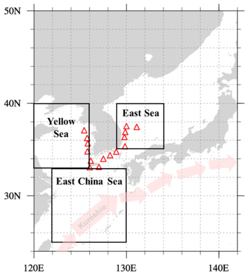
Figure 1.
Spatial distribution of marine buoys (red triangles) around the Korean Peninsula and the ocean sectors involved. Arrows indicate the Kuroshio current.
The purpose of this study is to produce a satellite-based oceanic turbulent heat flux dataset optimized for the ocean around the Korean Peninsula, and to make it so it can be utilized for further research on the intercorrelation between typhoon and ocean heat flux over the region. To achieve this goal, using satellite-based air–sea variables and the coupled ocean–atmosphere response experiment (COARE) bulk algorithm [12], oceanic SHF and LHF around the Korean Peninsula were calculated and evaluated during the period 2014–2019. In addition, temporospatial variations in satellite-based oceanic turbulent heat flux during two typhoons, Soulik (2018) and Francisco (2019), were also investigated to elucidate the relationship between fluctuations in oceanic heat flux and typhoon intensity.
The data used in this study and typhoon cases are introduced in Section 2. Methods for producing air–sea variables and calculating sensible and latent heat fluxes using the bulk algorithm are described in Section 3. Section 4 presents the results of the calculation of oceanic turbulent heat flux and the temporospatial distribution of SHF and LHF around the Korean Peninsula. Variations in SHF and LHF accompanying typhoon intensity changes are investigated in Section 4. Section 5 provides a summary and conclusion.
2. Data
Figure 1 shows the study area and three ocean sectors, YS (32–38°N, 120–126°E), ES (35–40°N, 129–134°E), and ECS (25–32°N, 122–130°E), for producing and analyzing oceanic SHF and LHF in this study.
2.1. Satellite Data
To produce air–sea variables for calculating oceanic turbulent heat flux, satellite-measured 10 m neutral wind speed (UN; m s−1), atmospheric water vapor (W; mm), and sea surface temperature (Ts; °C) were used. All the satellite data used in this study were obtained from remote sensing systems (RSS).
Daily products of UN and W were from four remote sensors: the Advanced Microwave Scanning Radiometer2 (AMSR2) on the Global Change Observation Mission-Water (GCOM-W) [24]; the Global Precipitation Measurement (GPM) Microwave Imager (GMI) [25]; WindSat on Coriolis [26]; and the Special Sensor Microwave Imager/Sounder (SSMIS) on the Defense Meteorological Satellite Program (DMSP) F16–18 [27]. The satellite products of RSS provide observation data with a spatial resolution of 0.25° × 0.25° and the individual grid point has the satellite overpass time. The valid ranges of UN and W data are 0–50 m s−1 and 0–75 mm, respectively. The daily Ts came from the optimally interpolated sea surface temperature (OISST) product, which is derived from microwave satellite sensors such as AMSR-2, WindSat, GMI, etc. It provides the same spatial resolution with UN and W, and has a valid range of −3.0 to 34.5 °C.
2.2. Marine Buoy Data
Sea surface temperature, air temperature, wind speed, and humidity measured by 15 marine buoys operated by the Korean Meteorology Administration (KMA) around the Korean Peninsula (Figure 1) were used to produce and evaluate satellite-based air–sea parameters and turbulent heat flux. Daily mean air–sea variables were derived from hourly mean measurements. Sea surface temperature, air temperature, humidity, and wind speed were measured at about −0.3 m, 3.4 m, and 3.7 m, respectively.
2.3. Typhoons
The Soulik (2018) and Francisco (2019) typhoons were selected for the analysis of temporospatial fluctuations in SHF and LHF during typhoons. Typhoon Soulik began to develop on 16 August 2018, over the ocean ~260 km northwest of Guam. By 22 August, the intensity of Soulik had reached a stage of “very strong (wind speed of 44–54 m/s)”, according to the typhoon intensity criteria of KMA, with a central pressure of 950 hPa and maximum wind speed of 43 m s−1. Soulik weakened rapidly after the maximum stage, with the maximum wind speed decreasing to 12 m s−1 within 30 h [28]. Typhoon Francisco began to develop on 2 August 2019, over the ocean ~1120 km northeast of Guam. It grew up to “strong (wind speed of 33–44 m/s)”, and was the first typhoon after Judy of 1989 to make landfall on the Korean Peninsula even after landing in Japan.
Typhoon tracks (latitude and longitude) and intensity (central pressure and maximum wind speed) were obtained from the Regional Specialized Meteorological Center’s (RSMC) best track data.
3. Methods
3.1. Production of Air–Sea Variables
Daily mean air–sea variables were generated by averaging all satellite measurements in a day over each grid having a spatial resolution of 0.25° × 0.25°. Each grid point has seven observations per one day on average for the analysis period and study area. The wind speed provided by RSS is not actual wind speed, but neutral wind speed (UN) at 10 m. Therefore, to convert the UN to actual wind speed (U), we obtained a correction factor by comparing the actual and neutral wind speeds at buoy sites at a height of 10 m. The height-corrected wind speed values at buoy sites were calculated from COARE algorithm. The correction factor was 0.9070, which means the actual wind was weaker than the neutral wind by about 3% on average during our study period. Although the bias between actual and neutral wind depends on location and season [29], this study tried to produce heat flux based on satellite data as much as possible. Sea surface temperature was produced directly by satellite observation, so satellite-derived OISST Ts values were used to calculate oceanic turbulent heat flux after their validation by comparison with marine buoy measurements.
Atmospheric water vapor, meaning total precipitable water in units of mm, W, is strongly correlated with atmospheric specific humidity (Qa) [30,31,32,33]. Liu [30] estimated the monthly mean specific humidity using a fifth-order polynomial relationship with water vapor for global oceans, and Ruckstuhl et al. [32] defined a linear relationship between specific humidity and atmospheric water vapor. Bentamy [34] reported that the Qa estimated from satellite-measured brightness temperatures, which are sensitive to atmospheric water vapor, has a systemic error that increases with sea surface temperature. Kim et al. [35] therefore used Ts together with W for the more precise estimation of Qa, and obtained a strong consistency with the Qa from ocean buoys showing R2 = 0.94. Here, a third-order polynomial and an exponential relationship for W and Ts were adopted to produce a satellite-based Qa based via the empirical Equation (1):
where, a, b, c, d, and e are empirical coefficients derived from buoy-measured Qa and satellite-based W and values.
Satellite-based W, Ts, and U were used to estimate air temperature, Ta. Throughout the six years of buoy and satellite data, Ta had logarithmic and linear relationships with W and Ts, respectively. Similarly, Kim and Hong [36] found that Ts and Qa are related linearly and non-linearly, respectively, with Ta. We therefore attempted to construct a non-linear regression relationship between satellite-based Ts and W for estimating Ta (), but this involved a systemic error at high wind speeds. Satellite-based Ta was finally produced using Equation (2), based on the pre-determined relationships:
The empirical coefficients a, b, c, and d were obtained using buoy-measured Ta and satellite-derived Ts, W, and U. To determine the empirical coefficients of Equations (1) and (2), a function of the non-linear regression analysis in the Statistical Package for the Social Sciences program was utilized.
3.2. COARE 3.5 Bulk Algorithm
The COARE algorithm is based on the bulk aerodynamic equation, and v 3.0 [12] has been used widely for calculating oceanic SHF and LHF from air–sea variables based on in situ and remote-sensing observations (e.g., [13,16,17]). Brunke et al. [37] compared the accuracies of 12 bulk algorithms and reported that COARE is one of the most accurate algorithms. COARE 3.5, released in 2013, was applied here in the calculation of oceanic SHF and LHF. The parameters used in COARE 3.5 have been validated by comparison with large in situ datasets covering 16,000 h of measurements [38].
Sensible and latent heat fluxes were calculated by the COARE bulk algorithm using Equations (3) and (4).
where is atmospheric density (kg m−3), is the specific heat of air (J kg−1), is the latent heat of evaporation (J kg−1), and are transfer coefficients of sensible and latent heat, is wind speed (m s−1), and and are the differences in temperature (°C) and specific humidity (g/kg−1) between air and the sea surface. The specific humidity at the sea surface level is considered to be a humidity which is saturated by as much as 98% in a condition of corresponding sea surface temperature. SHF and LHF increase with air–sea differences in temperature, humidity and wind speed. Here, a positive flux indicates heat transfer from ocean to air.
4. Results and Discussion
4.1. Evaluation of Satellite-Based Air–Sea Variables and Turbulent Heat Flux
A comparison of daily mean satellite- and buoy-measured U and Ts during 2014–2019 is shown in Figure 2. Satellite-based wind speeds are strongly correlated with buoy-measured data (R2 = 0.80), with a considerable amount of data clustered around the 1:1 line (Figure 2a). Their statistical errors (Root Mean Square Error (RMSE) of 1.54 m s−1 and Mean Bias Error (MBE) of −0.40 m s−1) compared to the buoy-measured U might have been caused by the high temporal variability in wind speed and the limited number of satellite observations for specific grid points for any single day. The Ts values from satellites and buoys are more strongly correlated (R2 = 0.97; RMSE = 0.98°C; MBE = 0.12°C) because the diurnal variation in sea surface temperature is low due to the high specific heat of water (Figure 2b).
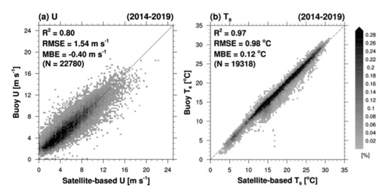
Figure 2.
Comparison of daily mean (a) wind speed (U, m s−1) and (b) sea surface temperature (Ts, °C) derived from satellite and buoy observations during the period 2014–2019. The dashed line is the 1:1 line. The color scale represents the density (%) of the data points.
The empirical coefficients in Equations (1) and (2) for estimating Qa and Ta are listed in Table 1 and Table 2, and comparisons between buoy- and satellite-derived Qa and Ta values are shown in Figure 3. There was strong correlation between these variables, with R2 values of 0.90 and 0.91 for Qa and Ta, respectively, and RMSE (and MBE) values of 1.78 g kg−1 (0.01 g kg−1) and 2.28°C (0.00°C), respectively. For Qa, the RMSE was 2.42 g/kg when only W was used in the estimation of Qa (not shown), but decreased to 1.78 g kg−1 by adding Ts as a related factor. The R2 and MBE also improved from 0.82 and 0.05 g kg−1 to 0.90 and −0.01 g kg−1, respectively. In addition, there are inconsistencies in the Ta comparison below ~15°C compared to the higher temperature range. This might be from the variation in the relationship between Ta and satellite-derived meteorological parameters (i.e., Ts, W, and U) according to variations in marine environment by season. Therefore, we clarify that there remains room for improvement in the estimation of satellite-based near-surface temperature in future studies.

Table 1.
Empirical coefficients for estimating Qa and Ta.
Table 2.
Root Mean Square Error (RMSE) and Mean Bias Error (MBE) between satellite- and buoy-based air–sea variables (U, Ts, Qa, Ta) and oceanic turbulent heat fluxes (SHF and LHF) for each season.
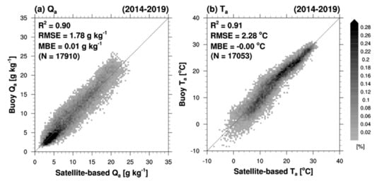
Figure 3.
Comparison of daily mean (a) specific humidity (Qa) and (b) air temperature (Ta) derived from satellite and buoy observations during the period 2014–2019. The dashed line is the 1:1 line. The color scale represents the density (%) of the data points.
Daily SHF and LHF values for the ocean around the Korean Peninsula were retrieved for the period 2014–2019 using satellite-based air–sea variables and the COARE 3.5 bulk algorithm. A comparison between satellite- and buoy-based SHF and LHF values at all buoy sites is shown in Figure 4. The SHF and LHF have R2 values of 0.72 and 0.79 between the two datasets, with RMSE (and MBE) values of 31.88 W m−2 (1.10 W m−2) and 49.76 W m−2 (−6.50 W m−2), respectively. The dispersion of the data from the 1:1 line can be explained by uncertainties in the satellite-based near-surface meteorological parameters (i.e., Ta and Qa). Zhou et al. [39] reported that errors in SHF and LHF from OAFlux are dominantly caused by inaccurate air temperature and specific humidity, respectively, by comparing the turbulent heat fluxes with those from flux tower observations. With increasing errors in Ta and Qa, the errors of SHF and LHF increased. In particular, they mentioned that the sensitivity of errors to Ta and Qa were larger in the winter season when the turbulent heat flux was large. Therefore, the uncertainties in satellite-based variables and turbulent heat fluxes were investigated seasonally.
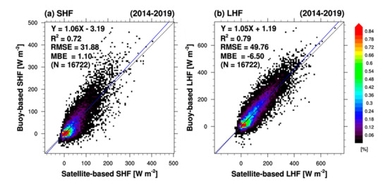
Figure 4.
Comparison between satellite-derived and buoy-based (a) sensible heat flux (SHF) and (b) latent heat flux (LHF) at all buoy sites during the period 2014–2019. Dashed and blue lines indicate the 1:1 line and regression line, respectively. The color scale represents the density (%) of the data points.
The statistical errors in air–sea variables and SHF and LHF estimations for seasonal and total datasets are shown in Table 2. The RMSE values for SHF and LHF are in the ranges of 12.71–47.48 W m−2 and 41.12–59.39 W m−2, respectively. The MBE of the SHF varies with the season, showing underestimations in winter (−19.87 W m−2, December–February) and overestimations in spring (13.39 W m−2, March–May). This is possibly due to the positive (1.58 °C) and negative (−1.21 °C) bias in Ta during winter and spring, respectively, because of the SHF being affected by the air–sea temperature difference (Equation (3)). That is, the deviation in the data from the 1:1 line above 100 W m-2 in the comparison of SHF (that is, the lower satellite-based SHF compared to that from the buoy measurements) came from the positive bias of Ta estimation in the winter season (Figure 4a). The LHF had positive and negative MBE values in spring–summer (4.26–10.04 W m−2) and autumn–winter (−16.43 to −24.72 W m−2), respectively. The seasonal LHF bias may be explained by the MBE values of the Qa estimation. The under- and overestimation of Qa causes large and small air–sea humidity differences, respectively, resulting in the over- and underestimation of LHF. This indicates the importance of the accuracy of the input data when calculating heat fluxes using the bulk algorithm.
Figure 5 shows the biases in the satellite-based air–sea variables and turbulent heat fluxes towards those from buoy-measurements as a function of wind speed. For the total period, the absolute errors of both fluxes increased with increasing U (Figure 5a,b). This might be caused partly by the uncertainty of satellite observation under high wind speed conditions. During the potential high-impact weather period (July–October), characterized by the frequent invasion of tropical storms into the Korean Peninsula, while LHF errors have a similar distribution to that of the total period, the estimation of satellite-based SHF shows positively biased errors. Under the strong wind speed condition, the estimation of satellite Ta was negatively biased during the period (Figure 5c), resulting in the overestimation of SHF, whereas the Qa estimation error does not seem to be related to increasing wind speed (Figure 5d). These uncertainties that appeared in the potential high-impact weather period should be considered in any further usage of the satellite-based oceanic turbulent heat flux of this study.
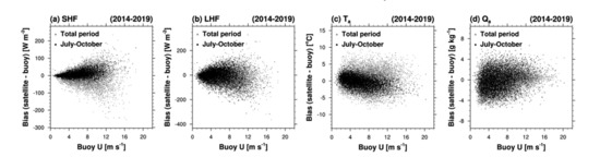
Figure 5.
Bias between satellite- and buoy- derived (a) SHF, (b) LHF, (c) Ta, and (d) Qa for buoy wind speed in the total period (gray dots) and for only June to October (black dots) during 2014–2019.
4.2. Characteristics of Oceanic Turblent Heat Fluxes around the Korean Peninsula
The spatial distributions of monthly mean SHF and LHF during 2014–2019 are shown in Figure 6. The SHF was no higher than 10 W m−2 over most of the study area during April–August, being almost zero at the YS and the ES in June and July. The LHF was transferred from ocean to atmosphere, showing positive values throughout the year, except for the area above 42°N in summer. From August, both heat fluxes increased sharply, from the high-latitude ES region for the SHF and the Kuroshio current region for the LHF. The SHF reached a maximum above 150 W m−2 in the Kuroshio current region, and above 40°N in the East Sea, while the LHF exceeded 320 W m−2 in January and December in the Kuroshio current region. Sim et al. [40] reported that a 25-year climatological distribution of the turbulent heat flux, obtained by combining eight datasets of oceanic turbulent flux, indicates a maximum LHF of ~332 W m−2 for the Kuroshio area during winter, with the SHF reaching 132 W m−2 in the ES and >140 W m−2 in the vicinity of Russia. The feature in the vicinity of Russia was explained by the high wind speeds of the region in the previous study.
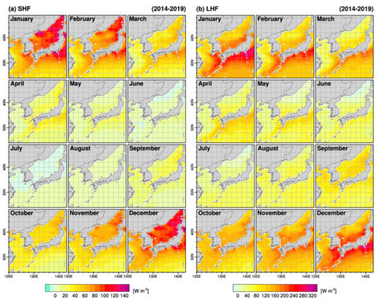
Figure 6.
Monthly mean (a) SHF and (b) LHF during 2014–2019 around the Korean Peninsula.
Monthly variations in air–sea variables and turbulent heat fluxes in the YS, ES, and ECS during the period 2014–2019 are shown in Figure 7 and Table 3. The SHF and LHF were low during the warm season and high in the cold season over the whole area (Figure 7g,h and Table 3). The SHF had little spatial variability during May–September, but the ES had a distinctly higher SHF (93 W m−2) in December than the YS and ECS (63 W m−2) (Figure 7g). This might have been due to a large air–sea temperature difference (ΔT) caused by greater water depth, low air temperatures in high-latitude regions, and high wind speeds during winter in the ES (Figure 7a–c,e). A greater water depth causes less temperature reduction in cold seasons and a smaller annual range of sea surface temperatures [41] (Figure 7b), resulting in relatively high ΔT in the cold season.
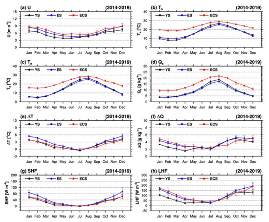
Figure 7.
Monthly mean air–sea parameters ((a) U, (b) Ts, (c) Ta, (d) Qa, (e) ΔT, and (f) ΔQ) and turbulent heat fluxes ((g) SHF and (h) LHF) in the YS (black), ES (blue) and ECS (red). Vertical error bars are standard deviations for six years.
Table 3.
Monthly mean of SHF and LHF in the YS, ES, and ECS for the period 2014–2019.
The LHF was comparable in the three ocean areas during May–October, but during November–April the YS had smaller LHF values than the other areas (Figure 7h). The YS had a wide annual range of Ts due to its shallow depth, with a small difference in specific humidity (ΔQ) during November–April (Figure 7d,f). Moreover, wind speeds in the YS region were significantly lower than those in the ES and ECS except for July–October (Figure 7a). The lower ΔQ and U values of the YS resulted in lower LHF values than in the ES and ECS. Kim et al. [35] and Oh et al. [42] suggested that the LHF is sensitive to wind speed, particularly during cold seasons. During September–October, the LHF values of the three sectors are comparable, despite the lower ΔQ of the ECS. These similar LHF values may be derived from the higher wind speed in ECS than in the other regions (Figure 7a). Variations in satellite-based air–sea variables and turbulent heat flux imply that the characteristics of the energy exchange between atmosphere and ocean vary significantly with the marine environment.
4.3. Changes in Oceanic Turbulent Heat Flux During Typhoons
In this Section, spatial and temporal variations in SHF and LHF were investigated during the two typhoons, Soulik (2018) and Francisco (2019), to find the relationships between oceanic turbulent heat flux and typhoon intensity.
4.3.1. Typhoon Soulik (2018)
Typhoon Soulik (2018) was generated on 16 August 2018, and intensified to a maximum wind speed of 43 m s−1 and central pressure of 950 hPa when passing the southern coast of Kyushu, Japan, on 21 August (Figure 8a). On 22 August, it slowed, and its intensity began to drop. Migration speed fell to a minimum of 4 km h−1 and the typhoon interacted strongly with the underlying ocean, resulting in a rise of cold water and its rapid weakening [28].
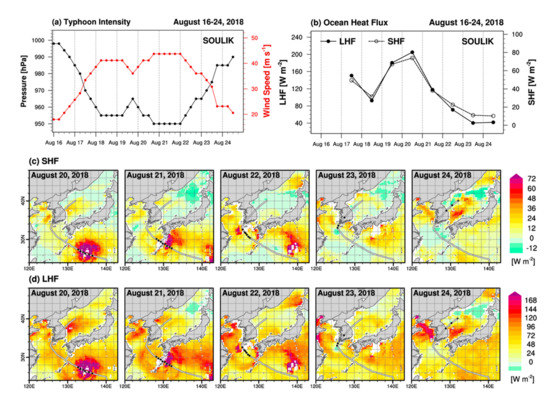
Figure 8.
Time series of (a) typhoon intensity (central pressure and wind speed) and (b) LHF and SHF, which are averaged for the area within 2° of the center; and spatial distribution of daily mean (c) LHF and (d) SHF during typhoon Soulik, 2018. Gray lines are typhoon trajectory.
The time series of the satellite-based daily mean oceanic heat flux around the center of the typhoon is shown in Figure 8b. The LHF was as high as 200 W m−2 around the typhoon on 20 August when it neared its maximum intensity. With the decrease in LHF and SHF, Soulik began to weaken, and the LHF was about 40 W m−2 on 23 August when the greatest weakening occurred. Variations in SHF and LHF during the typhoon can also be seen from the spatial distribution shown in Figure 8c,d. Because the meteorological parameters (i.e., U, W, and Ts) derived from satellite observation are not valid in heavy rain conditions [24,25,26,27], there are missing points near the center of the typhoon. Moreover, satellite-based sea surface temperature performance is degraded by extremely strong wind speed conditions [43,44]. Nevertheless, it can be seen that the turbulent heat fluxes around the typhoon were strengthened in the spatial distribution maps. The LHF, which remained high around Soulik during its northwest migration, was reduced to zero on 23 August at the west of Jeju Island. Park et al. [28] reported that the LHF at the center of the typhoon, computed from the air–sea variables of the modern-era retrospective analysis for research and applications, fell to negative values as it passed to the west of Jeju Island. Our ocean turbulent heat flux derived from satellite observations well reproduced the turbulent heat exchanges during the typhoon. The SHF varied similarly to the LHF, although the former is related more to typhoon rainband structure than to intensity [6]. The effect of SHF on typhoons needs to be investigated through an additional typhoon case analysis in further study.
4.3.2. Typhoon Francisco (2019)
Typhoon Francisco made landfall on the Korean Peninsula after passing through the Japanese Archipelago. Francisco gradually developed from 2 August 2019, being intensified to a maximum wind speed of 36 m s−1 and central pressure of 970 hPa on 5 August (Figure 9a). The SHF and LHF remained high before the typhoon moved into the Kuroshio current area (Figure 9c,d) because of the high sea surface temperature in the area, which is essential for strengthening and maintaining typhoon intensity. The LHF around Francisco decreased from 77 W m−2 on 3 August to 61 W m−2 on 4 August, and then increased to 67 W m−2 while passing through the Kuroshio area on 5 August (Figure 9b,d). At that time, the typhoon intensity reached a maximum (Figure 9a), and maintained a “strong” status until just before landfall in Japan. After landfall ~110 km northwest of Kagoshima on 6 August, the typhoon weakened rapidly due to surface friction; however, it was not extinguished and made landfall on the Korean Peninsula, with heavy rain and strong winds, and with a total precipitation of 128 mm and wind gusts of up to 25 m s−1. In the Kuroshio current area, the ocean heat flux, which was high before the typhoon arrived, dropped during the period of 3–6 August. The passage of the typhoon caused a cold-wake in the sea surface temperature, which resulted from stirring by strong winds near the sea surface, causing decreases in the difference between air and sea temperature and specific humidity. As a result, the transfer of turbulent heat from sea to air dropped after the passage of the typhoon. Typhoons are thus not only affected by oceanic turbulent heat flux in terms of intensity and structure, but can change the amount and distribution of air–sea energy exchange before and after passage.
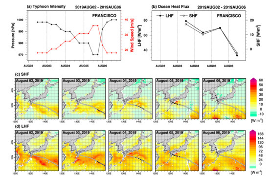
Figure 9.
Time series of (a) typhoon intensity (central pressure and wind speed) and (b) LHF and SHF, which were averaged for the area within 2° of the center; and spatial distribution of daily mean (c) LHF and (d) SHF during typhoon Francisco, 2019. Gray lines are typhoon trajectory.
5. Summary and Conclusions
Oceanic sensible and latent heat fluxes over the ocean around the Korean Peninsula were calculated using the COARE 3.5 bulk algorithm and meteorological products from GCOM-W/AMSR2, GPM/GMI, Coriolis/WindSat, and DMSP/SSMIS during the period 2014–2019. Of the four air–sea variables U, Ts, Qa, and Ta, U was obtained from satellite-measured UN with a conversion factor. Qa was estimated from non-linear relationships with W and Ts, and Ta was estimated on the basis of relationships with W, Ts and U. The determinant coefficients, R2, between satellite- and buoy-derived variables were in the range of 0.81–0.97. Oceanic SHF and LHF, computed using the bulk algorithm and satellite-based air–sea variables, were evaluated by comparison with heat fluxes computed from buoy-measured variables, with SHF and LHF having R2 values of 0.72 and 0.79, RMSE values of 31.87 and 49.35 W m−2, and MBE values of 1.99 and −4.03 W m−2, respectively. Seasonal statistical variables demonstrated the importance of accuracy in input data in the calculation of turbulent heat flux from the bulk algorithm. In addition, more precise correction of satellite-measured neutral wind speed to actual wind speed should be done in expanded studies in the future, for calculating reliable turbulent heat flux.
Both the SHF and LHF had lower values in warm seasons than in cold seasons. The LHF was from ocean to air throughout the year in most regions, and the SHF was below zero (from atmosphere to ocean) during June–July in the YS and ES regions. As the cold season approached, the SHF and LHF began to increase from high-latitude regions and from the Kuroshio current region, respectively. In the ES, the air–sea temperature difference (ΔT) was greater than that in the YS and ECS during the cold season because of the greater water depth, which possibly caused the difference in SHF by ocean area. The LHF was influenced predominantly by the air–sea humidity difference. Due to the shallow depth of the YS, the sea surface temperature decreased significantly during April–November, resulting in a lower ΔQ and lower LHF than in the ES and ECS. However, during September–October, although the YS and ES had higher ΔQ than the ECS, the LHF was similar in the three ocean areas because of the high wind speeds in the ECS region. Air–sea heat exchange thus varies with marine environment factors, such as water depth, sea surface temperature, and wind speed.
Distributions of air–sea heat exchange during typhoons Soulik (2018) and Francisco (2019) were investigated using satellite-derived SHF and LHF. The ocean heat flux was high when the typhoon maintained its strong intensity, and the typhoons weakened with the decreasing SHF and LHF in the northern ECS region. Soulik had the sharpest weakening when the LHF at its center became negative. Typhoon Francisco met high oceanic turbulent heat flux and reached its maximum intensity in the ECS region. Because most of the typhoons affecting the Korean Peninsula travel over the ECS region before landing and/or exerting their influence, the monitoring of turbulent heat flux over the region is important. Furthermore, it is also shown that both the SHF and LHF in the Kuroshio current region decreased after typhoon Francisco passed.
Analyses of the temporospatial distributions of satellite-based turbulent heat flux thus confirm that typhoons can be affected by oceanic heat flux in terms of strength, but can also affect the distribution of air–sea heat exchange. However, the influence of vertical wind shear must also be considered in the analysis of the association between oceanic turbulent flux and typhoon intensity, as typhoon intensity is greatly affected by vertical wind shear. Therefore, further observation- and simulation-based studies of typhoons are required to elucidate the relationship between oceanic heat flux and typhoon intensity, with more typhoon cases during the late summer and early autumn seasons. For instance, Fujiwara et al. [45] performed sensitivity experiments for typhoon Chaba (2010) to investigate the remote contribution of the Kuroshio current to tropical cyclone development by controlling the LHF over the Kuroshio current region, and found the importance of moisture supply for typhoon intensification.
The satellite-based oceanic SHF and LHF products discussed here may aid the understanding of air–sea turbulent heat exchange, and may be utilized in the construction of regional energy budgets around the Korean Peninsula. Flux products from previous studies (e.g., J-OFURO, GSSTF, OAFlux, etc.) provided the turbulent heat fluxes for the global ocean, but took some air–sea variables from reanalysis datasets. For example, to calculate heat flux, the GSSTF [14] and OAFlux [16] obtained near-surface temperatures from NCEP reanalysis data, and J-OFURO [13] used NCEP sea surface temperature data. The usage of reanalysis data lowers the utilization of monitoring heat flux in near-real time. This study only uses variables derived from satellite observations. Therefore, the methodology of producing air–sea variables could be utilized properly in the near-real time calculation of oceanic heat flux for monitoring the distribution of flux change. It may also be used to derive comparative data to produce more accurate flux information for the Kuroshio current region, where there are significant discrepancies in existing flux datasets [39,46]. Our methods also can be used to monitor oceanic heat flux during typhoons in the summer season, and to improve our understanding of the relationship between oceanic heat flux and typhoon intensity and structure. Moreover, through surface heat flux data assimilation, the performance of forecasting typhoon intensity could be improved.
Author Contributions
Conceptualization, Y.G.L. and J.K.; methodology, Y.G.L. and J.K.; software, J.K.; validation, J.K.; formal analysis, J.K.; investigation, J.K.; resources, Y.G.L. and J.K.; data curation, Y.G.L. and J.K.; writing—original draft preparation, J.K.; writing—review and editing, Y.G.L. and J.K.; visualization, J.K.; supervision, Y.G.L.; project administration, Y.G.L.; funding acquisition, Y.G.L. All authors have read and agreed to the published version of the manuscript.
Funding
This research was funded by the grant (NRF-2018R1C1B6008223) from the National Research Foundation of Korea (NRF).
Institutional Review Board Statement
Not applicable.
Informed Consent Statement
Not applicable.
Acknowledgments
The authors would like to thank the RSS for providing the satellite datasets, the RSMC for the provision of best-track data for typhoons and the KMA for providing the marine buoy data.
Conflicts of Interest
The authors declare no conflict of interest.
References
- Rodgers, E.B.; Olson, W.S.; Karyampudi, V.M.; Pierce, H.F. Satellite-Derived Latent Heating Distribution and Environmental Influences in Hurricane Opal (1995). Mon. Weather Rev. 1998, 126, 19. [Google Scholar] [CrossRef]
- Bao, J.-W.; Wilczak, J.M.; Choi, J.-K.; Kantha, L.H. Numerical Simulations of Air–Sea Interaction under High Wind Conditions Using a Coupled Model: A Study of Hurricane Development. Mon. Weather Rev. 1986, 128, 2190–2210. [Google Scholar] [CrossRef]
- Li, W. Modelling air-sea fluxes during a western Pacific typhoon: Role of sea spray. Adv. Atmos. Sci. 2004, 21, 269–276. [Google Scholar] [CrossRef]
- Wu, L.; Wang, B.; Braun, S.A. Impacts of Air–Sea Interaction on Tropical Cyclone Track and Intensity. Mon. Weather Rev. 2005, 133, 3299–3314. [Google Scholar] [CrossRef]
- Chen, S.; Li, W.; Lu, Y.; Wen, Z. Variations of latent heat flux during tropical cyclones over the South China Sea: Variations of latent heat flux during tropical cyclones. Met. Apps. 2014, 21, 717–723. [Google Scholar] [CrossRef]
- Ma, Z.; Fei, J.; Huang, X.; Cheng, X. Contributions of Surface Sensible Heat Fluxes to Tropical Cyclone. Part I: Evolution of Tropical Cyclone Intensity and Structure. J. Atmos. Sci. 2015, 72, 120–140. [Google Scholar] [CrossRef]
- Ma, Z. Examining the contribution of surface sensible heat flux induced sensible heating to tropical cyclone intensification from the balance dynamics theory. Dyn. Atmos. Ocean. 2018, 84, 33–45. [Google Scholar] [CrossRef]
- Businger, J.A. Evaluation of the Accuracy with Which Dry Deposition Can Be Measured with Current Micrometeorological Techniques. J. Clim. Appl. Meteorol. 1986, 25, 1100–1124. [Google Scholar] [CrossRef]
- Mason, P. Atmospheric Boundary Layer Flows: Their Structure and Measurement; Kaimal, J.C., Finnigan, J.J., Eds.; Oxford University Press: Oxford, UK, 1993. [Google Scholar]
- Gleckler, P.J.; Weare, B.C. Uncertainties in Global Ocean Surface Heat Flux Climatologies Derived from Ship Observations. J. Cimate 1997, 10, 18. [Google Scholar] [CrossRef]
- Kondo, J. Air-sea bulk transfer coefficients in diabatic conditions. Bound. Layer Meteorol. 1975, 9, 91–112. [Google Scholar] [CrossRef]
- Fairall, C.W.; Bradley, E.F.; Hare, J.E.; Grachev, A.A.; Edson, J.B. Bulk Parameterization of Air–Sea Fluxes: Updates and Verification for the COARE Algorithm. J. Clim. 2003, 16, 21. [Google Scholar] [CrossRef]
- Kubota, M.; Iwasaka, N.; Kizu, S.; Konda, M.; Kutsuwada, K. Japanese Ocean Flux Data Sets with Use of Remote Sensing Observations (J-OFURO). J. Oceanogr. 2002, 58, 213–225. [Google Scholar] [CrossRef]
- Chou, S.-H.; Nelkin, E.; Ardizzone, J. Surface Turbulent Heat and Momentum Fluxes over Global Oceans Based on the Goddard Satellite Retrievals, Version 2 (GSSTF2). J. Clim. 2003, 16, 18. [Google Scholar] [CrossRef]
- Shie, C.-L.; Chiu, L.S.; Adler, R.; Nelkin, E.; Lin, I.-I.; Xie, P.; Wang, F.-C.; Chokngamwong, R.; Olson, W.; Chu, D.A. A note on reviving the Goddard Satellite-based Surface Turbulent Fluxes (GSSTF) dataset. Adv. Atmos. Sci. 2009, 26, 1071–1080. [Google Scholar] [CrossRef]
- Yu, L.; Jin, X.; Weller, R. Multidecade Global Flux Datasets from the Objectively Analyzed Air-Sea Fluxes (OAFlux) Project: Latent and Sensible Heat Fluxes, Ocean Evaporation, and Related Surface Meteorological Variables; OAFlux Project Technical Report, OA-2008-01; Woods Hole Oceanographic Institution: Woods Hole, MA, USA, 2008; 64p. [Google Scholar]
- Andersson, A.; Fennig, K.; Klepp, C.; Bakan, S.; Graßl, H.; Schulz, J. The Hamburg Ocean Atmosphere Parameters and Fluxes from Satellite Data—HOAPS-3. Earth Syst. Sci. Data 2010, 2, 215–234. [Google Scholar] [CrossRef]
- Praveen Kumar, B.; Vialard, J.; Lengaigne, M.; Murty, V.S.N.; McPhaden, M.J. TropFlux: Air-sea fluxes for the global tropical oceans—Description and evaluation. Clim. Dyn. 2012, 38, 1521–1543. [Google Scholar] [CrossRef]
- Bourras, D. Comparison of Five Satellite-Derived Latent Heat Flux Products to Moored Buoy Data. J. Clim. 2006, 19, 6291–6313. [Google Scholar] [CrossRef]
- Chu, P.; Yuchun, C.; Kuninaka, A. Seasonal variability of the Yellow Sea/East China Sea surface fluxes and thermohaline structure. Adv. Atmos. Sci. 2005, 22, 1–20. [Google Scholar] [CrossRef]
- Emanuel, K.A. An Air-Sea Interaction Theory for Tropical Cyclones. Part I: Steady-State Maintenance. J. Atmos. Sci. 1986, 43, 585–605. [Google Scholar] [CrossRef]
- Jaimes, B.; Shay, L.K.; Uhlhorn, E.W. Enthalpy and Momentum Fluxes during Hurricane Earl Relative to Underlying Ocean Features. Mon. Wea. Rev. 2015, 143, 111–131. [Google Scholar] [CrossRef]
- Potter, H.; Drennan, W.M.; Graber, H.C. Upper ocean cooling and air-sea fluxes under typhoons: A case study. J. Geophys. Res. Ocean. 2017, 122, 9. [Google Scholar] [CrossRef]
- Wentz, F.J.; Meissner, T.; Gentemann, C.; Hilburn, K.A.; Scott, J. Remote Sensing Systems GCOM-W1 AMSR2 Daily Environmental Suite on 0.25 Deg Grid; Version 8.0; Remote Sensing Systems: Santa Rosa, CA, USA, 2014. [Google Scholar]
- Wentz, F.J.; Meissner, T.; Scott, J.; Hilburn, K.A. Remote Sensing Systems GPM GMI Daily Environmental Suite on 0.25 Deg Grid; Version 8.2; Remote Sensing Systems: Santa Rosa, CA, USA, 2015. [Google Scholar]
- Wentz, F.J.; Ricciardulli, L.; Gentemann, C.; Meissner, T.; Hilburn, K.A.; Scott, J. Remote Sensing Systems Coriolis WindSat Daily Environmental Suite on 0.25 Deg Grid; Version 7.0.1; Remote Sensing Systems: Santa Rosa, CA, 2013. [Google Scholar]
- Wentz, F.J.; Hilburn, K.A.; Smith, D.K. Remote Sensing Systems DMSP SSMIS Daily Environmental Suite on 0.25 Deg Grid; Version 8; Remote Sensing Systems: Santa Rosa, CA, USA, 2012. [Google Scholar]
- Park, J.; Yeo, D.; Lee, K.; Lee, H.; Lee, S.; Noh, S.; Kim, S.; Shin, J.; Choi, Y.; Nam, S. Rapid Decay of Slowly Moving Typhoon Soulik (2018) due to Interactions with the Strongly Stratified Northern East China Sea. Geophys. Res. Lett. 2019, 46, 14595–14603. [Google Scholar] [CrossRef]
- Kara, A.B.; Wallcraft, A.J.; Bourassa, M.A. Air-sea stability effects on the 10 m winds over the global ocean: Evaluations of air-sea flux algorithms. J. Geophys. Res. 2008, 113, C04009. [Google Scholar] [CrossRef]
- Liu, W.T. Statistical Relation between Monthly Mean Precipitable Water and Surface-Level Humidity over Global Oceans. Mon. Weather Rev. 1986, 114, 1591–1602. [Google Scholar] [CrossRef]
- Hsu, S.A.; Blanchard, B.W. The relationship between total precipitable water and surface-level humidity over the sea surface: A further evaluation. J. Geophys. Res. 1989, 94, 14539. [Google Scholar] [CrossRef]
- Schulz, J.; Schluessel, P.; Grassl, H. Water vapour in the atmospheric boundary layer over oceans from SSM/I measurements. Int. J. Remote Sens. 1993, 14, 2773–2789. [Google Scholar] [CrossRef]
- Ruckstuhl, C.; Philipona, R.; Morland, J.; Ohmura, A. Observed relationship between surface specific humidity, integrated water vapor, and longwave downward radiation at different altitudes. J. Geophys. Res. 2007, 112, D03302. [Google Scholar] [CrossRef]
- Bentamy, A.; Grodsky, S.A.; Katsaros, K.; Mestas-Nuñez, A.M.; Blanke, B.; Desbiolles, F. Improvement in air–sea flux estimates derived from satellite observations. Int. J. Remote Sens. 2013, 34, 5243–5261. [Google Scholar] [CrossRef]
- Kim, J.; Lee, Y.G.; Park, J.D.; Sohn, E.H.; Jang, J.-D. Calculation and Monthly Characteristics of Satellite-based Heat Flux Over the Ocean Around the Korea Peninsula. Korean J. Remote Sens. 2018, 34, 519–533. [Google Scholar] [CrossRef]
- Hong, G.-M.; Kwon, B.-H.; Han, Y.-H.; Kim, Y.-S. Estimation of marine meteorological parameters from the satellite data. Int. Geosci. Remote Sens. 2003, 4, 2254–2256. [Google Scholar] [CrossRef]
- Brunke, M.A.; Fairall, C.W.; Zeng, X.; Eymard, L.; Curry, J.A. Which Bulk Aerodynamic Algorithms are Least Problematic in Computing Ocean Surface Turbulent Fluxes? J. Clim. 2003, 16, 17. [Google Scholar] [CrossRef]
- Edson, J.B.; Jampana, V.; Weller, R.A.; Bigorre, S.P.; Plueddemann, A.J.; Fairall, C.W.; Miller, S.D.; Mahrt, L.; Vickers, D.; Hersbach, H. On the Exchange of Momentum over the Open Ocean. J. Phys. Oceanogr. 2013, 43, 1589–1610. [Google Scholar] [CrossRef]
- Zhou, F.; Zhang, R.; Shi, R.; Chen, J.; He, Y.; Wang, D.; Xie, Q. Evaluation of OAFlux datasets based on in situ air–sea flux tower observations over Yongxing Island in 2016. Atmos. Meas. Tech. 2018, 11, 6091–6106. [Google Scholar] [CrossRef]
- Sim, J.-E.; Shin, H.-R.; Hirose, N. Comparative Analysis of Surface Heat Fluxes in the East Asian Marginal Seas and Its Acquired Combination Data. J. Korean Earth Sci. Soc. 2018, 39, 1–22. [Google Scholar] [CrossRef]
- Oh, S.-Y.; Jang, S.-W.; Kim, D.-H.; Yoon, H.-J. Temporal and Spatial Variations of SL/SST in the Korean Peninsula by Remote Sensing. J. Fish. Mar. Sci. Educ. 2012, 24, 333–345. [Google Scholar] [CrossRef]
- Oh, H.M.; Ha, K.J.; Shim, J.S.; Hyun, Y.K.; Yun, K.S. Seasonal characteristics of turbulent fluxes observed at Ieodo Ocean Research Station. Atmosphere 2007, 17, 421–433. [Google Scholar]
- Dong, S.; Gille, S.T.; Sprintall, J.; Gentemann, C. Validation of the Advanced Microwave Scanning Radiometer for the Earth Observing System (AMSR-E) sea surface temperature in the Southern Ocean. J. Geophys. Res. 2006, 111, C04002. [Google Scholar] [CrossRef]
- Gentemann, C.L.; Wentz, F.J. Satellite Microwave SST: Accuracy, Comparisons to AVHRR and Reynolds SST, and Measurement of Diurnal Thermocline Variability. In Proceedings of the IEEE 2001 International Geoscience and Remote Sensing Symposium, Sydney, Australia, 9–13 July 2001; pp. 246–248. [Google Scholar] [CrossRef]
- Fujiwara, K.; Kawamura, R.; Kawano, T. Remote Thermodynamic Impact of the Kuroshio Current on a Developing Tropical Cyclone Over the Western North Pacific in Boreal Fall. J. Geophys. Res. Atmos. 2020, 125. [Google Scholar] [CrossRef]
- Hirose, N.; Lee, H.-C.; Yoon, J.-H. Surface Heat Flux in the East China Sea and the Yellow Sea. J. Phys. Oceanogr. 1999, 29, 17. [Google Scholar] [CrossRef]


Publisher’s Note: MDPI stays neutral with regard to jurisdictional claims in published maps and institutional affiliations. |
© 2020 by the authors. Licensee MDPI, Basel, Switzerland. This article is an open access article distributed under the terms and conditions of the Creative Commons Attribution (CC BY) license (http://creativecommons.org/licenses/by/4.0/).