Article

Using Satellite Data to Optimize Wheat Yield and Quality under Climate Change

1
Department of Geography and Environment, Bar-Ilan University, Ramat-Gan 5290002, Israel
2
Department of Vegetable and Field Crop Research, Agricultural Research Organization, Gilat Research Center, Gilat 8531100, Israel
*
Author to whom correspondence should be addressed.
Remote Sens. 2021, 13(11), 2049; https://doi.org/10.3390/rs13112049
Submission received: 16 April 2021 / Revised: 18 May 2021 / Accepted: 20 May 2021 / Published: 22 May 2021
(This article belongs to the Section Environmental Remote Sensing)

Abstract

:
Climatic conditions during the grain-filling period are a major factor affecting wheat grain yield and quality. Wheat in many semi-arid and arid areas faces high-temperature stress during this period. Remote sensing can be used to monitor both crops and environmental temperature. The objective of this study was to develop a tool to optimize field management (cultivar and sowing time). Analysis of 155 cultivar experiments (from 10 growth seasons) representing different environmental conditions revealed the required degree-days for each Israeli spring wheat cultivar to reach heading (from emergence). We developed a Google Earth Engine (GEE) app to analyze time series of gap-filled 1 km MODIS land surface temperature (LSTcont). By changing the cultivar and/or emergence date in the GEE app, the farmer can “expose” each wheat field to different climatic conditions during the grain-filling period, thereafter enabling him to choose the best cultivar to be sown in the field with the right timing. This approach is expected to reduce the number of fields that suffer from heat stress during the grain-filling period. The app can be also used to assess the effects of different global warming scenarios and to plan adaptation strategies in other regions too.

Graphical Abstract

1. Introduction

Climatic changes are likely to impact food production and pose serious challenges to food security. Remote sensing can help agricultural systems to adapt measures to negate the adverse impacts of climate change [1]. Wheat (Triticum aestivum L.) is one of the vital cereal crops grown worldwide, providing the primary caloric and nutritional source for a significant portion of the human population [2]. In order to ensure food security, there is a need for strategies and policies for the mitigation of food shortages. Timely and accurate estimates of global crop production are also essential. The adaptability of wheat to a wide range of environments has been favored by allelic diversity in genes regulating growth habits [3] i.e., temperature (VRN genes) and photoperiod response (PPD genes). Climate conditions during the grain-filling period are a major factor affecting wheat grain yield and quality. Wheat in many semi-arid and arid areas is facing high-temperature stress during this growth period. This challenge will probably be relevant in other growing areas in the future. Climatic variation is considered a main factor affecting gluten quality within a given variety when tested across different sites and/or seasons [4,5,6]. Growing Degree Days (GDD) is a main factor in crop models which are used to support decision-making and planning, particularly in relation to climate change issues [7,8,9,10].
Remote sensing can be used to monitor environmental temperatures. Surface skin temperature observations (Tskin), as obtained from satellite data, provide useful climatological data of high spatial resolution and global coverage that enhances the traditional ground observations of surface air temperature (Tair). MODIS land surface temperature (LST) products retrieved from thermal infrared bands have an accuracy of <1 °C in the range from −10 to 50 °C. Using MODIS data for LST retrieval improves the quality of the LST product and the diurnal feature in the product due to better temporal, spatial and angular coverage of clear-sky observations [11]. The 1 km MODIS-LST data can reveal the large spatial variability of LST and potentially increase precision in forecasting and applying management strategies [12]. However, the relationship between Tskin and Tair may be complex as it is affected by numerous factors, such as vegetation cover, incoming solar radiation and wind [13]. Therefore, data must be treated with adequate procedures, taking into account the temporal variation, crop cover and phenology, etc. [14,15].
In Mediterranean rain-fed conditions, such as in Israel, the amount of rainfall and its distribution during the growing season has a marked influence on spring wheat yield and quality [4,5,16,17,18,19]. Drought or heat shock during the grain filling period results in smaller yields and test weight, due to kernel shriveling. Sowing is recommended in Israel in a window from 15 November to 15 December based on the short rainy season, an increasing water deficit and thermal stress during grain filling and a higher probability of chilling/frost in January–February during anthesis. In Israel, late-heading cultivars can be sown from November 1st, resulting in a high variation between the commercial field’s emergence and phenological stage. Furthermore, grain quality standards are not consistently met in any given year due to adverse weather, which is the overriding factor controlling grain yield, grain test weights and protein concentration [4]. Hence, the sowing date in each field should be determined precisely, based on the wheat genetic and air temperature considering the spatial variability. Reaching heading can be predicted in-season by modeling [20] or by remote sensing [21,22]. However, there is a gap of knowledge for predicting heading date pre-sowing in advance. The objective of this study is to develop, calibrate and validate algorithms for the retrieval of wheat heading stage using time series of satellite data. We used the Google Earth Engine (GEE) platform to provide non-expert stakeholders (farmers) with a tool for optimizing yield by choosing the best sowing date and cultivar.

2. Materials and Methods

In order to develop an algorithm that provides estimation of the heading date for a specific cultivar, given the field location and the emergence date, the following tasks are needed:
  • A table of GDD required to reach the heading stage from the emergence stage for each cultivar. This is described in Section 2.1.
  • To calculate GDD for each field. This is described in Section 2.2.
  • To disseminate the algorithm as a tool to all stakeholders (farmers and the scientific community). This is described in Section 2.3.

2.1. Wheat Fields

This study uses three datasets that contain the emergence and heading dates from different locations (Figure 1): one dataset from Gilat Research Center is used for calibration (Gilat-CAL), and two other datasets are used for validation: one from commercial wheat fields at Saad (Saad-VAL), and another from 28 wheat variety test experiments across Israel (CVexp-VAL).
  • The Gilat-CAL dataset contains data from 76 wheat variety test experiments from ten growth seasons (2008–2017) at Gilat Research Center. Each experiment included several spring bread wheat cultivars spanning the phenological range of Israeli elite germplasm. Each experiment typically included 8–15 cultivars, with a total of 22 different cultivars. The dataset comprises more than 1500 heading date records, taken by one person (DJ. Bonfil). Daily meteorological data from Gilat meteorological station was used. The meteorological station was typically within 1 km distance from the field, with a maximum distance of 2.5 km. This data set was used to calculate the GDD (with a temperature threshold of 0 °C) and the number of days from emergence to heading (E–H) for each cultivar.
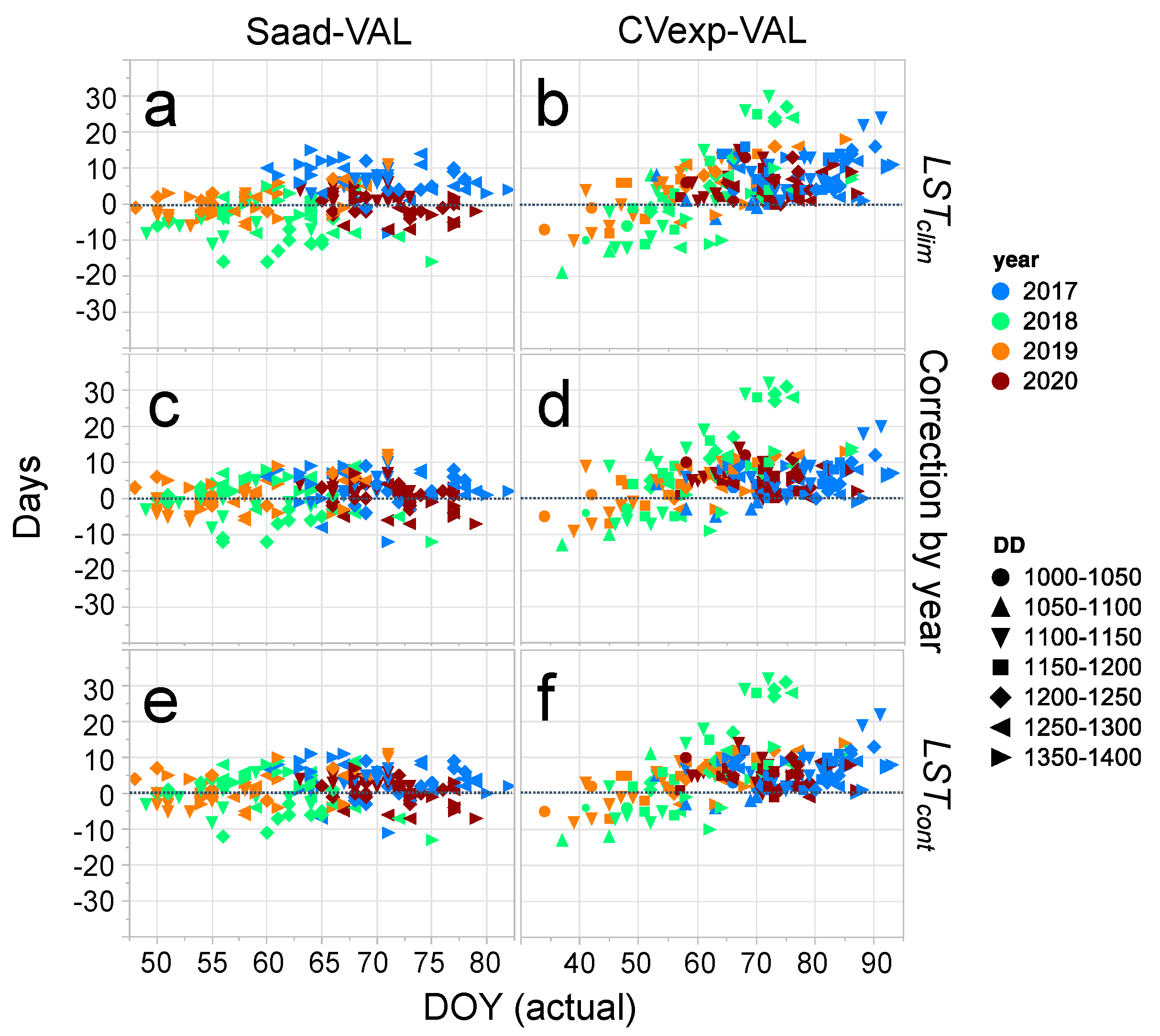
  • The Saad-VAL dataset contains data from commercial wheat fields at Saad (Saad, Saad-BH, Figure 1) from four growth seasons (2017–2020). Four cultivars (Amit, Gadish, Kitain and Ruta) represent most of the fields (180 out of 206 records). A single person (Y. Nir, the farmer) reported all heading data in the Saad-VAL dataset.
  • The CVexp-VAL dataset contains data from 28 wheat variety test experiments established across Israel from four growth seasons (2017–2020). The fields are located in the northern and southern growing Israeli areas (Figure 1). The dataset includes 188 records from 19 cultivars. Eleven cultivars represent 163 out of 188 fields. In this dataset, heading data for each experiment were taken by the local extension person that runs the experiment.

2.2. Satellite and Numerical Weather Prediction Model Data

MODIS onboard Terra and Aqua polar-orbiting sun-synchronous satellites provide global coverage daily LST at 1 km spatial resolution at 10:30 (Terra) and 1:30 (Aqua) AM/PM local time. We used 2002–2020 Aqua LST data since it better represents the maximum and minimum diurnal LST. The MYD11A1 V6 product [23] was used to retrieve the seasonal behavior of LST in cloud-free conditions.
Numerical weather prediction (NWP) models provide surface temperature regardless of cloud cover. We used NCEP Climate Forecast System Version 2 (CFSv2) NWP model surface air temperature 2 m above ground at a spatial resolution of 0.2° [24] to fill gaps in the LST dataset due to cloud cover [25]. Forecasts are initialized four times per day (0000, 0600, 1200 and 1800 UTC). The data is available from 1979 to the present.
Temporal Fourier Analysis (TFA) was used to derive the climatological temperatures of the satellite (MODIS LST) and model (CFSv2) temperatures. The TFA describes the seasonal cycles of temperature in terms of annual, bi-annual and tri-annual components (or “harmonics”), each described by its phase and amplitude. These Fourier harmonics may be recombined, providing a smoothed signal, which is regarded here as the climatological expected temperatures:
L S T c l i m ( t ) = L S T ¯ + i = 1 n A i c o s ( ω i t φ i )
where t is the Julian date, LSTclim(t) is the climatological temperature at time t, L S T ¯ is the mean annual temperature, A i is the amplitude of the ith harmonic component and n is the number of harmonic components. We used here the first three harmonics (n = 3), following Scharlemann et al. [25] and Lensky and Dayan [12]. φ i is the phase and ω i is the frequency ( ω i = 2 π i / 365 ) of the ith harmonic component. TFA was applied on both MODIS LST and CSFv2 surface (2 m air) temperature to derive the climatological temperature and the anomaly (the deviation of the actual temperature from the climatological temperature).
Surface temperature at a specific time and date can be regarded as being composed of two components: (a) the long-term mean (climatology), and (b) the deviation from that mean due to the weather (anomaly). Shiff et al. [26] proposed a method based on these principles and provided a continuous (gap-filed) LST dataset (LSTcont) based on satellite (MODIS LST) and model (CFSv2) temperature data. Figure 2a presents the Shiff et al. [26] continuous (gap-filed) LST dataset for two wheat-growing seasons (November–March, 2017–2018). The 2017 LST time-series shows an accumulated negative anomaly of −46 GDD, whereas 2018 shows an accumulated positive anomaly of 119 GDD. As a result, simulation of E–H from 1 December 2017 was 8 days shorter than in 2018 (Figure 2b).

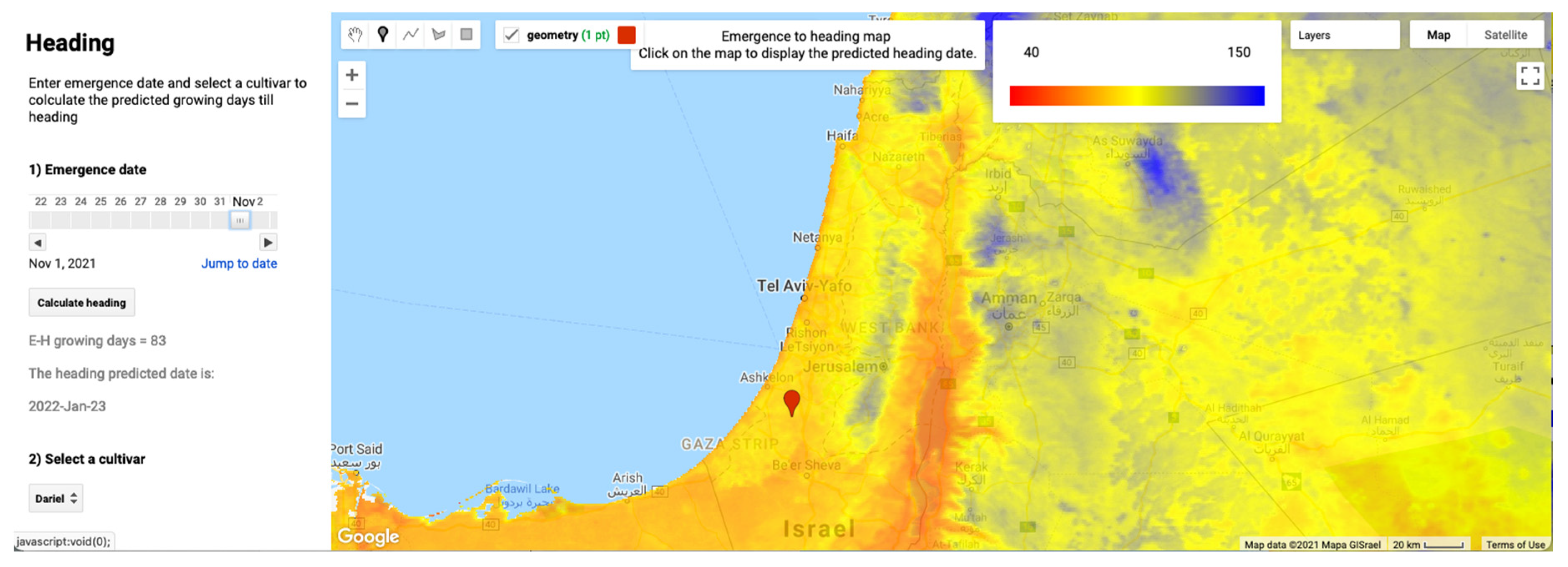
2.3. Google Earth Engine (GEE)

Google Earth Engine (GEE) is a parallel computation service platform for advanced image analysis that hosts a variety of remote sensing and geospatial datasets [27]. Both products (MODIS LST and CFSv2) are available on the GEE platform. GEE leverages its cloud computing service for analysis capabilities of time series data, which are otherwise heavy consumers of time and computation resources. Our research uses ~20 years’ time-series of daily datasets that are all hosted on the GEE platform to calculate climatological LST (LSTclim) and continuous gap-filled LST (LSTcont). GEE also helps researchers to easily disseminate their products to other users and researchers, which enabled us to provide code and a web app, for the benefit of farmers and the science community. The present study provides a GEE web app that enables optimization of yield by providing the farmer with the expected heading date for each combination of field, cultivar and emergence date (see Supplementary Materials).

3. Results

A large difference in wheat heading dates, from late December until April, was found in the wheat fields. Differences in meteorological conditions, genotypes, sowing and emergence dates explain this variability. Since all cultivars are spring wheat that do not require vernalization, the emergence to heading (E–H) period was mainly affected by temperature and photoperiod (day length) response. Early and late emergence exposes the wheat to warmer conditions and longer days, therefore decreasing the E–H period (for all cultivars). We calculated the growing degree days (GDD, the accumulated daily average temperature above a base temperature threshold of 0 °C) for the E–H period. The GDD (E–H) decreases as the emergence date occurs later than mid-December (Figure 3), since late emergence exposes the wheat to warmer conditions and longer days, therefore decreasing the E–H period (for all cultivars). Phenological ranking between cultivars is kept across the environments; cultivars Yuval (Dariel) are the earliest (latest) with GDD E–H of 1000 (1385 °C), respectively. The calculated GDD for each cultivar can be seen in Figure 3. The following five cultivars have been determined for the app development: Very early, Early, Intermediate, Late and Very late (1000, 1100, 1200, 1300 and 1400 °C, respectively).
Usually, heading of the earliest emerging experiment occurred under cooler conditions (Figure 4). In the 2017–2018 growing season stress conditions (high temperatures) prevailed during the heading and grain-filling period, where the late phenology cultivars faced very high temperatures above 40 °C. Similar behavior was observed each season, with warmer conditions associated with later crop heading.
The Heading GEE web application (https://shilosh.users.earthengine.app/view/emergence2heading, accessed on 21 May 2021) is based on pre-computed daily climatological MODIS LST (LSTclim) at a resolution of 1 km for the entire world. The interface includes a map to select the field and to see the predicted heading map, a calendar for selecting the emergence date and a drop-down list to select the cultivar (Figure 5). The user can select the emergence date and cultivar and visualize a map of the predicted number of days to heading (E–H). The user can then click on any point on the map and get the date of the predicted heading at that point.
During the 2017–2020 growing seasons, heading date estimations have been validated by two datasets: (a) from one farmer (his own fields) and (b) from the extension service advisers who established experiments across different growth conditions. Both achieved similar correlation (R2 0.53–0.6), high bias (15–18) and SEP of 6 to 7 days (Figure 6a,b and Table 1). Since there was high variation between the prevailed air temperatures along the four validation growing seasons, each season exhibits a different relation (Figure 6a,b). Adding the “year” effect improved the Saad-VAL dataset model to a correlation of 0.82, 2017 > 2020 > 2019 > 2018 (day of year (DOY) 70.5, 66.8, 61.5 and 59.4 respectively). A smaller improvement was shown by the CVexp-VAL data set with a correlation of only 0.7 by accounting the year effect, 2017 = 2018 = 2020 > 2019 (DOY 69.1, 68.4, 68.3 and 63.7 respectively). Using LSTcont resulted in a very similar performance compared to the yearly corrected data (Figure 6e,f, Figure 7 and Figure 8e,f and Table 1).
GEE app accessibility enables farmers to use the GEE heading app in the growing seasons since 2019 for planning sowing, cultivar X field X date (i.e., Genotype X Environment) using the climatological LST (LSTclim). Heading during warmer (cooler) seasons is expected to be earlier (later) than predicted when using LSTclim. Decision support during the season should include updated GDD. Using actual LST data (LSTcont) reduced the bias from 15.2 to 3.5 days in Saad-VAL, and from 17.9 to 11.4 days in CVexp-VAL (Table 1). R2 increased from ~0.56 to ~0.7; SEP decreased in Saad-VAL to 4.7 days. Moreover, the range of the difference decreased and reached mean ± 6 or 8 days for 80% of the fields, and ± 3 or 5 days for 50% of the fields, Saad-VAL and CVexp-VAL respectively (Figure 8c,d). LSTcont solves most of the trend shown for CVexp-VAL (Figure 8e,f), where the difference between the estimated and actual heading was related to timing: underestimation for earlier heading and overestimation for late heading. One of the CV-experiment data can be determined as outlier (all cultivars), as their DOY was recorded at about day 70, while according to the temperature it should have occurred one month earlier. Still, the mean difference distribution in the CVexp-VAL data is higher than 0, showing underestimation of the GEE application.
Temperatures are expected to rise due to climate change. To characterize how climate change could potentially impact the E–H period length, we evaluated future projections from the NASA Earth Exchange Global Daily Downscaled Projections (NEX-GDDP) ensemble [28], using the Coupled Model Intercomparison Project 5 (CMIP5 [29]) under the Representative Concentration Pathway 4.5 (RCP4.5) emission scenario, with the Australian Community Climate and Earth-System Simulator (ACCESS1-0). Figure 9 shows the projected changes on three cultivar types (Very early, Intermediate and Very late) for the period 2010–2099. The E–H period length on Gilat is expected to be shorten by 11 days with the Very late cultivar until the end of the century.

4. Discussion

Crop development is affected by temperature and is therefore a key factor in many crop models. The ability to use temperature data from space opens a new era. However, most models use air temperature, measured 2 m above the land surface, while Earth observations provide land surface temperature. Our results show that LST can be used without any transformation during the winter, which is the wheat growing season in Israel. These results are in accordance with previous studies [14,30,31]. In other growth seasons, adjustments between GDD from meteorological stations and from satellites will probably be needed, especially for summer crops. In addition, LSTcont enables using near to real-time MODIS-LST data, so LST can be incorporated into in-season decision support systems and/or crop models. However, LSTcont cannot predict future temperatures, therefore LSTcont can only provide GDD up to the current time, while a farmer who wants to plan the right sowing date and cultivar for the next season is limited to the use of LSTclim only. LSTcont enables using LST even in cloudy conditions, though validation is needed for growing areas where clouds persist for long periods.
Spatial temperature variations are small in some growing areas but can be very high in others. For example, variations between Saad fields (Saad-VAL) are small, while the CVexp-VAL dataset is based on high variation in growth conditions (Figure 1). Moreover, even for the Saad-VAL dataset, rain and/or irrigation creates high variation in the temperatures that the crops are exposed to during the different growth stages resulting in variance in emergence dates. The most important result achieved in this study is that the GEE based algorithm can forecast the heading date of each cultivar in every field. Therefore, it was used immediately for planning sowing, cultivar X field X date (i.e., G X E) by Israeli farmers.
Several factors can affect the accuracy, where “date determination” is the most important. Under good germination conditions, the emergence date can be easily determined (±1 day). However, hard conditions due to water stress, bad seed bed (large clods), variation in sowing depth and others can lead to different determination of the emergence date by different persons. Determining the heading date itself is challenging as not all plants reach this stage at the same day. Moreover, under high stand conditions differentiation between the main stem spike and tillers cannot be done. Hence, the significance of the heading date for the same field is somehow fuzzy. In the case where one person determines all fields, the date, emergence and heading, determination would be more consistent. Therefore, validation based on Saad-VAL reached better accuracy than CVexp-VAL which was monitored by more than one person.
Most inaccuracies in the Saad-VAL dataset are within 0 ± 5 days (Figure 8e), while for the CVexp-VAL most are within 5 ± 5 days (Figure 6f). The 5 day bias can mainly be attributed to the heading determination. Heading stages have been determined in the Gilat-CAL and Saad-VAL datasets when about 100% of the plants reached this stage and the emergence of the main tiller ear was complete, but not the tillers’ ears, while most extension advisors determine the heading date when emergence of about 80% of the whole field’s (including tillers) ears is complete. As tillers’ ears usually emerge a few days later, this explains the 5 day bias between the two validation sets. Crop modeling to predict phenology within season using real-time data reached a similar accuracy of ±3–7 days [20]. Our results exhibit that degree days can be used with similar accuracy, but more importantly, GDD can be used out of season—and even pre-season—to assist decision making.
The LST data has a spatial resolution of 1 km per pixel. Most fields are smaller than 1 km, thus the estimated field LST represents a mixed pixel. The spatial resolution can be improved using fusion schemes with Landsat data to 30 m [32,33]. However, the fusion procedure requires time and computation resources, and since the 1 km data have been found sufficient, there is no need to improve the spatial resolution.
Other sources of inaccuracy can be related to the Gilat-CAL dataset. Although calibration has been done by one person, and all data were collected from one area, for a few cultivars insufficient data was available. Consequently, their GDD requirement was not accurate enough, leading to miscalculation by the GEE-heading app.
The main benefit of using the GEE-heading app would be achieved by reducing the number of fields that suffer from heat stress during the grain-filling period. In case of an early rain event where germination occurs immediately after sowing, farmers can use the GEE-heading app to find the best sowing date for each field. In addition, the GEE-heading app can be used for other purposes as well. Estimation of the heading date can help growers reduce or prevent herbicide application that can cause damage during anthesis. The same is the case for the application of liquid nitrogen as late top-dressing.
Data can be used for interpretation and better understanding of crop development. In cases where heading in vivo exhibits a significant delay, it may be an indication for other stress limiting developments. Limiting factor identification can assist the specific or the following crop. It can be achieved by comparing the same cultivar grown in different locations and growth conditions.
The app can also be used to assess the effects of different global warming scenarios and to plan adaptation strategies in other regions too. Therefore, the environmental conditions during grain filling in a specific field can be modified by setting the optimal sowing date and cultivar. Sowing super early cultivars is a very important option to prevent warm and dry conditions during the grain filling period, encouraging breeders to release super early cultivars. However, shortening the growth season decreases the yield production potential, as crops absorb less radiation. Breeders can learn that in future seasons the growth period, emergence until heading, is expected to be shorter by 11 days (Figure 9). Therefore, they should include late phenology lines in their breeding programs too, that perhaps would not decrease yield production during shorter growth periods. All Israeli spring wheat cultivars (Figure 3) have identical PPD alleles resulting in similar responses to photoperiod. Hence, breeders may try to include other allele that will regulate development and delay the transition from vegetative apex to floral initiation or enlarge the stem elongation period.
Growth during warmer and cooler seasons is expected to be faster or slower than the seasonal average (during season). The next GEE app version should include within season updated in vivo GDD accumulation (i.e., LSTcont). In addition, heading app validation should be extended to different growth locations and conditions. Furthermore, since the precise field heading date determination is not clear and can differ between persons, validation should include data taken by many people. Another approach would be to test the heading app globally, first with spring wheat all over the world, and perhaps for winter wheat too.

5. Conclusions

The 1 km MODIS-LST data reveal the large spatial variability of LST. The GEE platform and time series of LST data were used to map the spatial variability for each field. The required GDD for each cultivar to reach heading from emergence was integrated into a GEE app and is available for use by farmers. By changing the cultivar and/or emergence date in the GEE app, the farmer can “expose” each wheat field to different climatic conditions during the grain filling period, thereafter enabling him to choose the best cultivar to be sown in the field. The main benefit would be achieved by reducing the number of fields that suffer from heat stress during the grain-filling period. The app can also be used to assess the effects of different global warming scenarios and to plan adaptation strategies in other regions as well. Therefore, the climate or at least the environment during the grain filling period can be modified.

Supplementary Materials

The Emergence to Heading GEE web application is available in: https://shilosh.users.earthengine.app/view/emergence2heading. The GEE web app’s code is publicly available through Github (https://github.com/shilosh/emergence2heading). GEE codes that calculate global LSTcont and LSTclim along with explanations on the usage of the code are publicly available through Github (https://github.com/shilosh/ContinuousLST.git).

Author Contributions

Conceptualization, D.J.B., S.S. and I.M.L.; methodology, D.J.B., S.S. and I.M.L.; software, D.J.B. and S.S.; validation, D.J.B. and S.S.; writing—original draft preparation, D.J.B. and S.S.; writing—review and editing, D.J.B., S.S. and I.M.L.; visualization, D.J.B., S.S. and I.M.L.; supervision, project administration and funding acquisition, D.J.B. and I.M.L. All authors have read and agreed to the published version of the manuscript.

Funding

This research was funded by the Chief Scientist of the Israeli Ministry of Agriculture and Rural Development, grant number #20-10-0066, and the Israeli Ministry of Science, Technology and Space, grant number 3-14675.

Acknowledgments

The authors would like to acknowledge Y. Nir from Kibbutz Saad and all Israeli extension advisors for their significant contribution to this study.

Conflicts of Interest

The authors declare no conflict of interest.

References

  1. Mutanga, O.; Dube, T.; Galal, O. Remote Sensing of Crop Health for Food Security in Africa: Potentials and Constraints. Remote Sens. Appl. Soc. Environ. 2017, 8, 231–239. [Google Scholar] [CrossRef]
  2. Shewry, P.R.; Hey, S.J. The Contribution of Wheat to Human Diet and Health. Food Energy Secur. 2015, 4, 178–202. [Google Scholar] [CrossRef] [PubMed]
  3. Distelfeld, A.; Li, C.; Dubcovsky, J. Regulation of Flowering in Temperate Cereals. Curr. Opin. Plant Biol. 2009, 12, 178–184. [Google Scholar] [CrossRef] [PubMed] [Green Version]
  4. Bonfil, D.J.; Abbo, S.; Svoray, T. Sowing Date and Wheat Quality as Determined by Gluten Index. Crop Sci. 2015, 55, 2294–2306. [Google Scholar] [CrossRef]
  5. Har-Gil, D.; Bonfil, D.J.; Svoray, T. Multi Scale Analysis of the Factors Influencing Wheat Quality as Determined by Gluten Index. Field Crops Res. 2011, 123, 1–9. [Google Scholar] [CrossRef]
  6. Moldestad, A.; Fergestad, E.M.; Hoel, B.; Skjelvåg, A.O.; Uhlen, A.K. Effect of Temperature Variation during Grain Filling on Wheat Gluten Resistance. J. Cereal Sci. 2011, 53, 347–354. [Google Scholar] [CrossRef]
  7. Miller, O.; Helman, D.; Svoray, T.; Morin, E.; Bonfil, D.J. Explicit Wheat Production Model Adjusted for Semi-Arid Environments. Field Crops Res. 2019, 231, 93–104. [Google Scholar] [CrossRef]
  8. Rosenzweig, C.; Elliott, J.; Deryng, D.; Ruane, A.C.; Müller, C.; Arneth, A.; Boote, K.J.; Folberth, C.; Glotter, M.; Khabarov, N.; et al. Assessing Agricultural Risks of Climate Change in the 21st Century in a Global Gridded Crop Model Intercomparison. Proc. Natl. Acad. Sci. USA 2014, 111, 3268–3273. [Google Scholar] [CrossRef] [Green Version]
  9. Schauberger, B.; Gornott, C.; Wechsung, F. Global Evaluation of a Semiempirical Model for Yield Anomalies and Application to Within-Season Yield Forecasting. Glob. Chang. Biol. 2017, 23, 4750–4764. [Google Scholar] [CrossRef]
  10. Xu, C.; Liu, H.; Williams, A.P.; Yin, Y.; Wu, X. Trends toward an Earlier Peak of the Growing Season in Northern Hemisphere Mid-Latitudes. Glob. Chang. Biol. 2016, 22, 2852–2860. [Google Scholar] [CrossRef]
  11. Wan, Z.; Zhang, Y.; Zhang, Q.; Li, Z.-L. Quality Assessment and Validation of the MODIS Global Land Surface Temperature. Int. J. Remote Sens. 2004, 25, 261–274. [Google Scholar] [CrossRef]
  12. Lensky, I.M.; Dayan, U. Detection of Finescale Climatic Features from Satellites and Implications for Agricultural Planning. Bull. Am. Meteorol. Soc. 2011, 92, 1131–1136. [Google Scholar] [CrossRef] [Green Version]
  13. Jin, M.; Dickinson, R.E. Land Surface Skin Temperature Climatology: Benefitting from the Strengths of Satellite Observations. Environ. Res. Lett. 2010, 5, 044004. [Google Scholar] [CrossRef] [Green Version]
  14. Blum, M.; Lensky, I.M.; Nestel, D. Estimation of Olive Grove Canopy Temperature from MODIS Thermal Imagery Is More Accurate than Interpolation from Meteorological Stations. Agric. For. Meteorol. 2013, 176, 90–93. [Google Scholar] [CrossRef]
  15. Kloog, I.; Chudnovsky, A.; Koutrakis, P.; Schwartz, J. Temporal and Spatial Assessments of Minimum Air Temperature Using Satellite Surface Temperature Measurements in Massachusetts, USA. Sci. Total Environ. 2012, 432, 85–92. [Google Scholar] [CrossRef] [Green Version]
  16. Bonfil, D.J.; Mufradi, I.; Klitman, S.; Asido, S. Wheat Grain Yield and Soil Profile Water Distribution in a No-Till Arid Environment. Agron. J. 1999, 91, 368–373. [Google Scholar] [CrossRef]
  17. Kafkafi, U.; Bonfil, D.J. Integrated Nutrient Management—Experience and concepts from the Middle East. In Integrated Nutrient Management for Sustainable Crop Production and Environmental Safety; Milkha, S.A., Grant, C.A., Eds.; Haworth Press, Inc.: Binghamton, NY, USA, 2008; pp. 523–565. [Google Scholar]
  18. López-Bellido, L.; Fuentes, M.; Castillo, J.E.; López-Garrido, F.J. Effects of Tillage, Crop Rotation and Nitrogen Fertilization on Wheat-Grain Quality Grown under Rainfed Mediterranean Conditions. Field Crops Re. 1998, 57, 265–276. [Google Scholar] [CrossRef]
  19. Turner, N.C. Further Progress in Crop Water Relations. In Advances in Agronomy; Sparks, D.L., Ed.; Academic Press: Cambridge, MA, USA, 1996; Volume 58, pp. 293–338. [Google Scholar]
  20. Wallach, D.; Palosuo, T.; Thorburn, P.; Gourdain, E.; Asseng, S.; Basso, B.; Buis, S.; Crout, N.; Dibari, C.; Dumont, B.; et al. How Well Do Crop Modeling Groups Predict Wheat Phenology, given Calibration Data from the Target Population? Eur. J. Agron. 2021, 124, 126195. [Google Scholar] [CrossRef]
  21. Pimstein, A.; Eitel, J.U.H.; Long, D.S.; Mufradi, I.; Karnieli, A.; Bonfil, D.J. A Spectral Index to Monitor the Head-Emergence of Wheat in Semi-Arid Conditions. Field Crops Res. 2009, 111, 218–225. [Google Scholar] [CrossRef] [Green Version]
  22. Sadeghi-Tehran, P.; Sabermanesh, K.; Virlet, N.; Hawkesford, M.J. Automated Method to Determine Two Critical Growth Stages of Wheat: Heading and Flowering. Front. Plant Sci. 2017, 8, 8. [Google Scholar] [CrossRef] [Green Version]
  23. Justice, C.O.; Townshend, J.R.G.; Vermote, E.F.; Masuoka, E.; Wolfe, R.E.; Saleous, N.; Roy, D.P.; Morisette, J.T. An Overview of MODIS Land Data Processing and Product Status. Remote Sens. Environ. 2002, 83, 3–15. [Google Scholar] [CrossRef]
  24. Saha, S.; Moorthi, S.; Wu, X.; Wang, S.; Nadiga, S.; Tripp, P.; Behringer, D.; Hou, Y.T.; Chuang, H.Y.; Iredell, M.; et al. Updated Daily. NCEP Climate Forecast System Version 2 (CFSv2) 6-Hourly Products. Available online: https://doi.org/10.5065/D61C1TXF (accessed on 20 February 2020).
  25. Scharlemann, J.P.W.; Benz, D.; Hay, S.I.; Purse, B.V.; Tatem, A.J.; Wint, G.R.W.; Rogers, D.J. Global Data for Ecology and Epidemiology: A Novel Algorithm for Temporal Fourier Processing MODIS Data. PLoS ONE 2008, 3, e1408. [Google Scholar] [CrossRef] [PubMed]
  26. Shiff, S.; Helman, D.; Lensky, I.M. Worldwide Continuous Gap-Filled MODIS Land Surface Temperature Dataset. Sci. Data 2021, 8, 74. [Google Scholar] [CrossRef] [PubMed]
  27. Gorelick, N.; Hancher, M.; Dixon, M.; Ilyushchenko, S.; Thau, D.; Moore, R. Google Earth Engine: Planetary-Scale Geospatial Analysis for Everyone. Remote Sens. Environ. 2017, 202, 18–27. [Google Scholar] [CrossRef]
  28. Thrasher, B.; Maurer, E.P.; McKellar, C.; Duffy, P.B. Technical Note: Bias Correcting Climate Model Simulated Daily Temperature Extremes with Quantile Mapping. Hydrol. Earth Syst. Sci. 2012, 16, 3309–3314. [Google Scholar] [CrossRef] [Green Version]
  29. Taylor, K.E.; Stouffer, R.J.; Meehl, G.A. An Overview of CMIP5 and the Experiment Design. Bull. Am. Meteorol. Soc. 2012, 93, 485–498. [Google Scholar] [CrossRef] [Green Version]
  30. Good, E.J. An in Situ-Based Analysis of the Relationship between Land Surface “Skin” and Screen-Level Air Temperatures. J. Geophys. Res. Atmos. 2016, 121, 8801–8819. [Google Scholar] [CrossRef]
  31. Lensky, I.M.; Dayan, U.; Helman, D. Synoptic Circulation Impact on the Near-Surface Temperature Difference Outweighs That of the Seasonal Signal in the Eastern Mediterranean. J. Geophys. Res. Atmos. 2018, 123, 11333–11347. [Google Scholar] [CrossRef]
  32. Agam, N.; Kustas, W.P.; Anderson, M.C.; Li, F.; Neale, C.M.U. A Vegetation Index Based Technique for Spatial Sharpening of Thermal Imagery. Remote Sens. Environ. 2007, 107, 545–558. [Google Scholar] [CrossRef]
  33. Rotem-Mindali, O.; Michael, Y.; Helman, D.; Lensky, I.M. The Role of Local Land-Use on the Urban Heat Island Effect of Tel Aviv as Assessed from Satellite Remote Sensing. Appl. Geogr. 2015, 56, 145–153. [Google Scholar] [CrossRef]
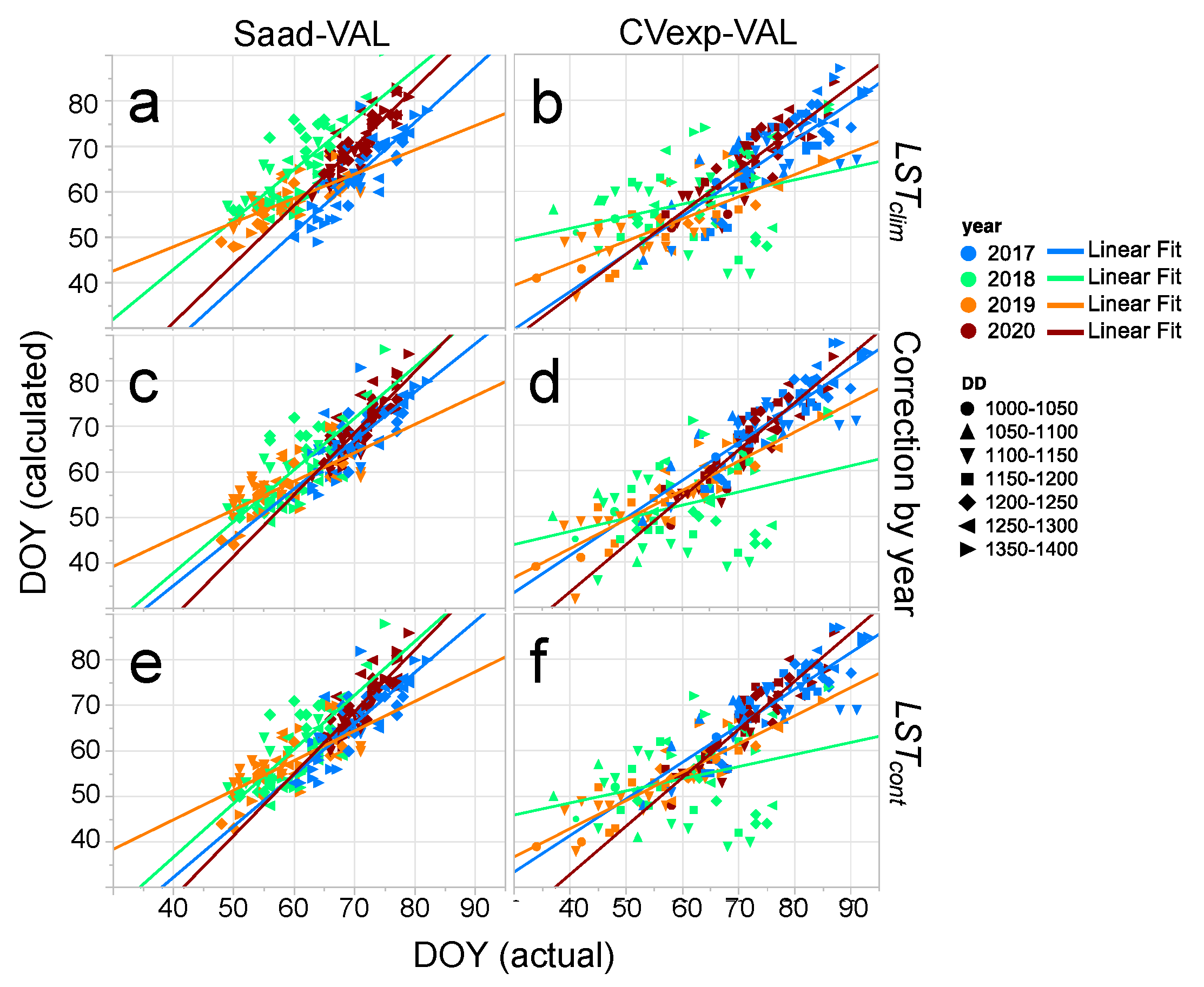
Figure 1. Mean MODIS LST (2002–2020) in Israel for (a) November, (b) December, (c) January and (d) February. The green points represent the locations of the wheat fields used for the calibration and validation datasets.
Remotesensing 13 02049 g001
Figure 2. (a) LST data from Gilat (Figure 1) is presented for two growing seasons: LSTcont for 2017 (blue), 2018 (red) and LSTclim (green). Positive/negative anomalies are colored in light red/blue. (b) The growing degree days (accumulated degree days with temperature threshold of 0 °C) are plotted for two emergence dates: November 1 and December 1. The differences between above average temperatures 2018 and below average 2017 resulted in eight days difference at heading for the very early cultivar and is marked as a double-headed arrow in mid-February.
Remotesensing 13 02049 g002
Figure 3. Gilat-CAL: GDD required from emergence till heading (E–H) period as affected by emergence date (from November 1st). Symbols represent different Israeli spring wheat cultivars.
Remotesensing 13 02049 g003
Figure 4. Average daily air temperatures—solid black line; grey shading—min to max, measured at Gilat (Figure 1) during the 2017–2018 growing season. LSTcont (black dotted line) represents skin temperature and therefore is warmer in the hot seasons than air temperature. In Israel’s winter (wheat spring cultivars growing season) LSTcont and air temperature are almost identical [14]. NDVI time-series of three cultivar experiments are plotted in green, emerged on November 28 (solid line), December 16 (dashed line) and January 11 (dotted line). Horizontal lines indicate the heading date period from the early to the late cultivars for the same emergence date.
Remotesensing 13 02049 g004
Figure 5. The interface of the Heading GEE web application. Here, based on the user input of 1 November as the emergence date and Dariel as the cultivar, presenting a map of Israel, Jordan and parts of Egypt and Syria with color scale of red to blue representing number of E–H days.
Remotesensing 13 02049 g005
Figure 6. Wheat field heading timing (Julian date starting from January 1) estimation using the GEE application vs. field monitoring in Saad-VAL (a,c,e) and CVexp-VAL (b,d,f). Symbol colors represent years and symbol shapes represent cultivars. Estimations shown in (a,b) use LSTclim, in (c,d) use a correction of yearly behavior and in (e,f) use LSTcont.
Remotesensing 13 02049 g006
Figure 7. A comparison between the heading DOY calculated by adding the “year” affect and the heading DOY that was calculated by LSTcont, which resulted in r² of 0.987 and RMSE of 1.153. Data was taken from both datasets (Saad-VAL and CVexp-Val).
Remotesensing 13 02049 g007
Figure 8. Heading days differences between field monitoring and 3 methods of calculation: LSTclim (a,b), Yearly correction (c,d) and LSTcont (e,f). The performance of yearly correction and the LSTcont in Saad-VAL (c,e) and CVexp-VAL (d,f) are very similar.
Remotesensing 13 02049 g008
Figure 9. Climate change predictions for temperature in Gilat (2010–2099) show decrease of heading date for very late, intermediate and very early wheat cultivars. Data from NASA Earth Exchange Global Daily Downscaled Climate Projections (NEX-GDDP).
Remotesensing 13 02049 g009
Table 1. Statistics for differences between wheat field heading Julian date estimation by LSTclim, Yearly correction and LSTcont at two validation sets vs. field monitoring.
Saad-VAL (n = 206)CVexp-VAL (n = 188)
LSTclimYearly CorrectionLSTcontLSTclimYearly CorrectionLSTcont
r0.7270.8500.8440.7730.8260.820
R20.5290.7230.7120.5980.6820.673
Bias15.1724.1823.56217.8919.01711.438
SEP5.7854.5944.7456.7906.7866.638
Publisher’s Note: MDPI stays neutral with regard to jurisdictional claims in published maps and institutional affiliations.

