Incorporating Persistent Scatterer Interferometry and Radon Anomaly to Understand the Anar Fault Mechanism and Observing New Evidence of Intensified Activity

Abstract

Interferometric Synthetic Aperture Radar (InSAR) monitors surface change and displacement over a large area with millimeter-level precision and meter-level resolution. Anar fault, with a length of ~200 km, is located in central Iran. Recent seismological studies on the fault indicated that it is approaching the end of its seismic cycle. Although a large earthquake is imminent, the mechanism of the fault is not well understood. Therefore, understanding and discovering the mechanism of Anar fault remains a challenge. Here, we present an approach of displacement fault analysis utilizing a combination of InSAR data obtained from the persistent scatterer interferometry (PSI) method and 178 Sentinel-1 images (ascending and descending) (2017–2020). We incorporated groundwater samples from 40 wells, radon concentration anomaly mapping, Global Positioning System (GPS), and 3D displacement measurement acquired over four years (2016–2020). We investigated and monitored the deformation of the fault plate’s behavior over the last three years (2017–2020) to explore new evidence and signature of displacement. The results show that the time series analysis in the fault range has an increasing displacement rate in all dimensions. We observed that the line-of-sight (LOS) displacement rate varied from −15 mm to 5 mm per year. Our calculations show that the E–W, N–S, and vertical displacement rates of the fault blocks are 2 mm to −2 mm, 6 mm to −6 mm, and 2 mm to −4 mm per year, respectively. An anomaly map of the radon concentration shows that the complete alignment of the high concentration ranges with the fault strike and the radon concentration increased on average from 23.85 Bq/L to 25.30 Bq/L over these three years. Therefore, we predict rising the radon concentration is due to the increase in activity which resulted in a deformation. Finally, our findings show that the Anar fault is an oblique and right-lateral strike-slip with a normal component mechanism. We validated the proposed method and our results by comparing the GPS field data and PSI measurements. The root mean square error (RMSE) of the PSI measurement is estimated to be 0.142 mm. Based on the supporting evidence and signature, we conclude that the Anar fault activity increased between 2017 and 2020.

1. Introduction

Monitoring the dynamic behavior of faults can play an important role in forecasting earthquakes’ imminence [1,2,3,4,5,6,7,8,9,10]. Various methods have been used to investigate the activity of faults, including geomorphological evidence, morphostructural analyses, and paleoseismology [11,12,13,14,15,16,17,18]. Today, with remote sensing science development, especially in radar imaging, a new door has been opened to study the displacement of the Earth’s crust [19,20]. The radar interferometry methods are increasingly used to study faults, earthquakes, subsidence, and other natural hazards [21,22,23,24,25,26,27]. Given the capability of radar images in determining the displacements on the ground surface over a certain period, these images can be used to monitor the changes made on the faults [28,29]. The early interferometric techniques used in the study of faults and the scatterings’ varied nature of ground surface phenomena would restrict the use of these methods over time [4,27,30]. Therefore, approaches such as the PSI technique for low displacement rate and a series of geological phenomena such as faults for lack of temporal correlation of pixels can be very helpful for deformation analysis [23,31].

Monitoring the displacement rate on fault plates can help forecast possible earthquakes [32,33,34]. Displacements accumulated on faults eventually move the main fault plates [1]. A schematic model of the accumulated displacement occurring at a point in a fault is presented by Mouslopoulou et al. (2009) [35] They showed that the displacement rate differs between long- and short-term intervals with the displacement rate of fault in short-term intervals varying from low to high. Hicks and Rietbrock (2015) [6] studied the seismic slip on an upper-plate normal fault. The authors analyzed how seismic data affect the earthquake and the Chilean subduction zone in 2011. Lu and Wang (2021) [34] demonstrated a post-seismic deformation with large subduction earthquakes and studied the independent evidence. They showed how the seaward post-seismic motion is deflecting upward at the edge of the cold forearc mantle wedge, thereby causing diagnostic uplift.

The increasing slip rate of the Anar fault temporarily indicates an increase in dynamic activity and a higher probability of earthquakes [35,36]. Therefore, a good approach to investigate the activity of faults is to monitor the short-term displacement and determine the displacement rate using radar image processing [8,15,32,37].

Moreover, scholars have used Time-Series InSAR (TS-InSAR) techniques to compensate for the conventional InSAR deficiencies [38,39]. Besides the approaches mentioned above, there are two main TS-InSAR approaches which utilize the time series of SAR images to extract the fault displacement and deformation. The first approach, Persistent Scatterer (PS) InSAR, concentrates on the pixels with temporal scattering steadiness. It extracts the time series deformation and fault displacement of the identified pixels based on their phase variation in the spatiotemporal domain [40,41]. Such methods, which are dedicated to tracking phase-stable scatterers’ deformation, have been successfully applied to urban areas [41]. However, in non-urban regions, especially vegetated areas and desert areas, it is difficult to find enough PSs for the regional deformation extraction. This is true for the Anar fault area. The second approach, the small-baseline subset (SBAS) InSAR, estimates the ground deformation using the interferograms with short spatial and temporal baselines [42,43]. This method is based on interferogram formation. This designed approach maximizes interferometric coherence for more distributed targets [40,44]. Consequently, researchers have mapped deformation with spatially dense observations [23,31]. Therefore, by using this approach, we can produce the time-series deformation characteristics of each identified object. The remote sensing and SBAS technique have been successfully applied to the time-series deformation extraction of earthquake, landslide, volcano, and permafrost. For example, Barnhar et al. (2020) [10] presented a detailed co-seismic surface-strain analysis for the 2019 earthquake in Ridgecrest, California. They used satellite optical imagery and derived three-dimensional high-resolution surface displacements. Then, they inverted deformation for the co-seismic surface-strain tensors.

In addition, some scholars have monitored the concentration of radon dissolved in the groundwater of the world’s seismic regions to obtain signs related to the activity of faults and the probability of imminent earthquakes [45,46,47,48]. Abnormal changes in radon concentration have been reported before major earthquakes [47,49]. Different atmospheric, terrestrial, and subsurface parameters (pressure, temperature, and groundwater stress) manage the process of radon emission from rocks into groundwater sources [50,51]. Measuring the concentration of radon dissolved in groundwater can pave the way to understand and recognize displacements in the Earth’s crust such as fractures and varied stress on fault plates. Recent studies showed a significant relationship between increasing radon concentrations dissolved in groundwater and the occurrence of some major earthquakes [49]. Additionally, the radon concentration distribution has been used to identify active faults and their expansion [52]. Due to the dense clay and sand cover around the Anar fault, researchers have not discovered the mechanism. However, we have been able to establish the type of fault mechanism from analyzing the 3D displacement measurement.

A few studies have been conducted on the Anar fault. Foroutan et al. (2012) [14] used paleoseismological studies to report the signs of three earthquakes above magnitude 7.0 throughout the history of this fault. According to the studies, the return period of large earthquakes was over, and the probability of their occurrence was very high [14,46]. Yamani et al. (2013) [46] only focused on morphotectonic evidence of Anar fault activity. The results of their study showed that the Anar fault was active, and there was a great deal of evidence of its activity in the late Holocene. Based on their approach, this study determines new evidence and signature on the intensified activity of Anar fault. In our work, we have addressed the gaps in previous studies of the Anar fault mechanism. In contrast to the previous studies which did not calculate the displacement, we attempted a detailed analysis of the fault displacement mechanism utilizing InSAR images. We monitored radon concentration anomaly and fault displacement behavior for three years from remote sensing data, incorporating groundwater samples of 40 wells and GPS measurements. In contrast, other studies expressed the relationship between radon and the fault but did not determine the behavior of displacement anomaly. Therefore, according to the studies, we estimated that the release of radon gas from rocks will also increase with the increase of fault activity. For this purpose, an attempt was made in this study to investigate this issue quantitatively. We used linear regression geostatistical techniques to determine the variable relationship between surface displacement and the amount of radon gas dissolved in groundwater. We constructed a regression model to predict the radon anomaly response using given predictors’ surface displacement.

Our study monitored process deformations and displacements around the south termination of the Anar fault for three years using the PSI method and GPS ground measurement. We analyzed the fault’s activity behavior by monitoring the variation of radon concentration dissolved in groundwater in the region. This study proposed a revised method and modified interpretation of the fault displacement mechanism utilizing 148 Sentinel-1 ascending and descending images (2017–2020). For the first time, the three following processes were combined: (i) three years (2017–2020) groundwater sampling, monitoring, and radon map generation; (ii) PSI, including differential interferogram and GPS measurement; and (iii) 3D map process including LOS displacement mapping.

The rest of the paper is organized as follows. Section 2 presents the study area, the Anar fault specifications, and the tectonic setting. We explain the method of research in Section 3. This section provides the dataset acquisition and explains the PSI method, azimuth offset, 3D displacement calculation, groundwater sampling, radon measurement, and anomaly mapping. We discuss the analysis and the results of this study in Section 4. Finally, we wrap up the results and discussion of this study and conclude the paper in Section 5.

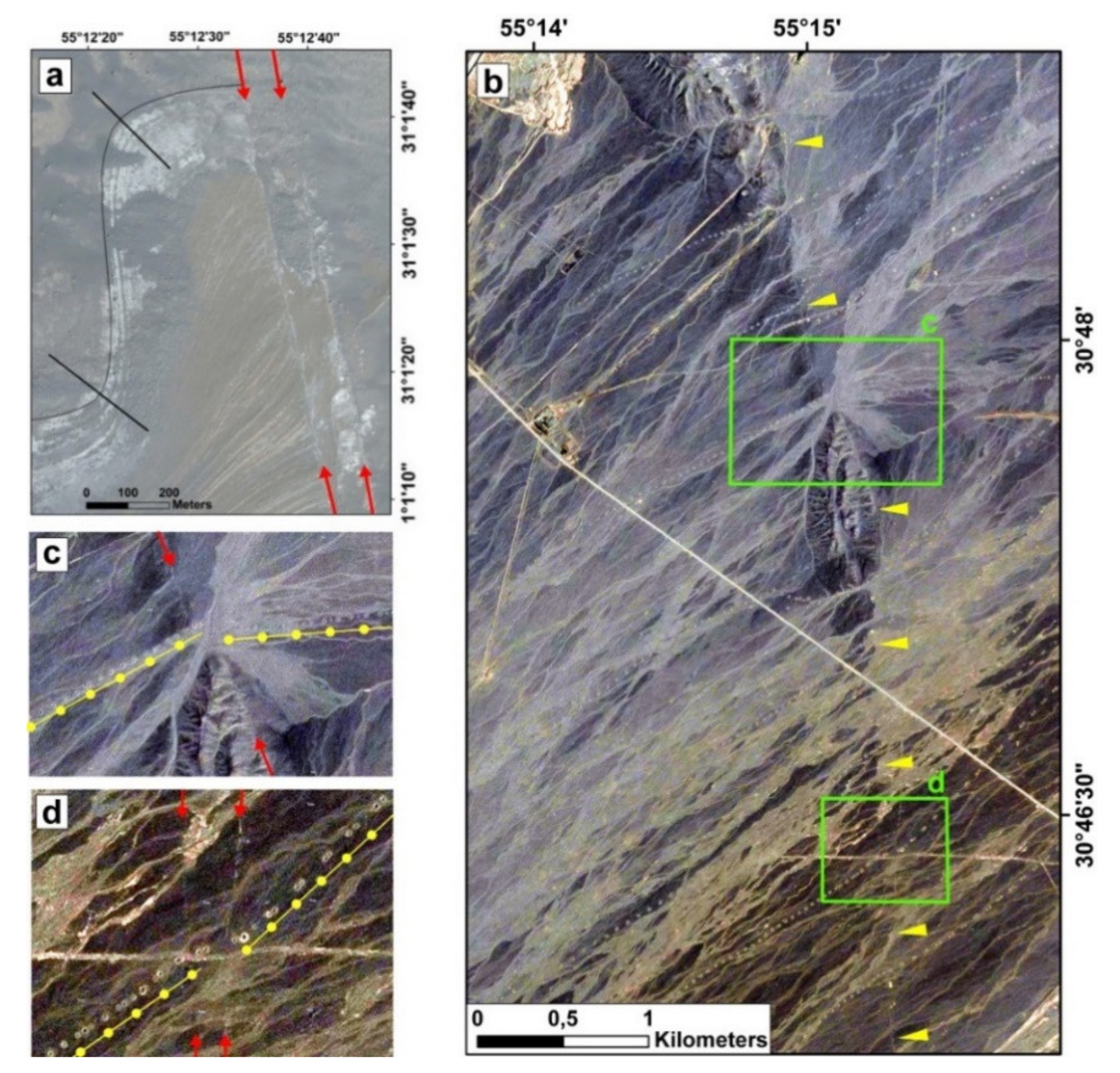
2. Study Area, Fault Specifications and Tectonic Setting

The study area of approximately 30 km² is located in the north of Kerman Province. Thirty kilometers of the 200 km Anar fault is located in the study area (Figure 1). Anar city, northwest of Rafsanjan, with its population of over 50,000 people, is located near this fault [53]. The study area has hot and dry regions in terms of climate, with the average annual rainfall not exceeding 100 mm. With the presence of many pistachio orchards in this region, there is irregular groundwater abstraction, and many wells have been dug.

Anar fault, with a length of approximately 200 km (Figure 2), is one of the active faults in Central Iran. The fault has a slip movement at 0.8 mm/year [14,54]. The northern part is in the mountainous region, and the southern part continues along the foothills to the Anar Salt Plan. Anar city is located in the south part, where the fault trace, ~30 m fault scarp, and displacement in streams are visible (Figure 2a–c). Due to the dense clay and sand cover around the fault, the mechanism in southern termination has not been determined by geomorphological evidence. Hence, both normal and reverse components may have created the scarp (Figure 2d,e). In this study, we were able to determine the type of right-lateral strike-slip and oblique fault mechanism.

Tectonic studies show that the Iranian plate has a high density of active and recent faults where large-scale horizontal motion occurs on narrow zones of major strike-slip faults [3,12,55]. Iran has a complex tectonic evolution dependent on the multistage history of the Tethys domain. The integration of smaller continental blocks of Gondwanan affinity to Eurasia (Afghan, Lut, and Central Iran subdivided into Tabas and Yazd blocks) has resulted from sequential closing and opening of the oceanic domains or back-arc and marginal basins. Closure of the Paleotethys is shown by ophiolitic remnants related to the accretion of Early Jurassic to Eurasia [12,56]. The Late-Cretaceous to Early Tertiary closure of several Neo-Tethys oceanic subductions is confirmed by the location of more continuous and younger sutures: Nain Baft among Sanandaj Sirjan and Central Iran to the south, Sabzevar (SB) among Eurasia and Central Iran to the north, and Sistan among Afghanistan and Lut to the east. Emplacement of Urumieh-Dokhtar arc occurred during Eocene-Oligocene, which is the source of many metal mineral resources, including large copper mines in Iran, and is dependent on the northward subduction of Neotethys oceanic plate under the Iran continent [57,58,59,60].

The activity rate of the strike-slip faults with NNW-SSE trend within the central Iran plate (e.g., Anar fault) and along the edges of Lut block (Gowk-Nayband, Neh -Kahurak-Zahedan) was dependent on the ongoing collisional stage. Thus, present slip rates of the strike-slip fault are important to the timing of the relief and regional kinematics evolution. Numerous studies in eastern and central Iran have recorded geomorphological expressions such as displaced, deformed, and deflected landforms along the active seismic faults. Geomorphologic scientists conducted early studies of active faulting in the Iran plateau [61]. The most recent studies of available data for active faulting are found in [14,62,63]. A few studies have been conducted on the active tectonics of Anar fault in the plain (e.g., Foroutan et al., 2012 [14]).

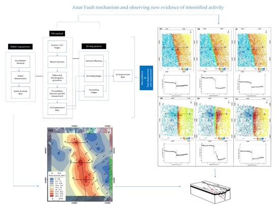
3. Data Acquisition and Methods

A total number of 178 ascending and descending scenes of Sentinel-1 TOPS mode interferometric wide swath (IW) in single-look complex (SLC) format were acquired between March 2016 and May 2020.

Table 1. Sentinel-1 image parameter.

Orbit Type	Orbit Number	Time Span	Number of Images	Number of Interferograms
Descending	488	March 2016–May 2020	81	80
Ascending	98	September 2016–May 2020	97	96

illustrates the Sentinel-1 image parameters. These images are freely available through the Copernicus Open Access Hub (https://scihub.copernicus.eu, accessed on 1 May 2020). We performed geometric corrections of range doppler terrain correction to reduce the distortion effects and prepare the data for the PS-InSAR. All of the descending and ascending slave images are co-registered to the master images captured on 21 July 2018 and 18 September 2018. We used external digital elevation model (DEM) data and the shuttle radar topography mission (SRTM) 30 m spatial resolution to eliminate terrain phase contributions. In addition, we attempted extensive field observations and utilized GPS measurements to monitor the displacement.

Our proposed approach was to combine the three processes in this study. They include (i) groundwater sampling, monitoring, radon measurement of three years (2017–2020), and anomaly mapping; (ii) PSI method and GPS measurements; and (iii) 3D map process using a combination of azimuth offsets and LOS measurements. We can see the proposed model in Figure 3. The authors processed and analyzed 178 InSAR Sentinel-1 SLC images using Snap opensource software, Delft object-oriented radar interferometric (DORIS), and StaMPS. The StaMPS analysis was applied to extract ground displacements from the acquired time series of 178 images. This study attempted three years of field observations and groundwater sampling to monitor radon concentration anomaly. We incorporated InSAR data from 2017–2020 and mapped the changes. We measured the radon concentration of groundwater samples adjacent to the Anar fault in the field three times every month from 2017 to 2020 by using a RAD 7 radon detector. The following sub-sections explain the three procedures mentioned above.

3.1. Persistent Scatterer Interferometry (PSI)

Due to the limitations of the conventional radar interferometry method, Ferretti et al. (2011) [40] presented the PSI method. The persistent scatterers are corner reflectors or natural features with stable backscattering characteristics over time and do not suffer from a lack of temporal correlations. These objects are mainly human-made. There are pixels in which a scatterer is dominant and behaves like a persistent point scatterer. Therefore, the persistent point scatterer reduces the amount of non-correlation significantly. We can measure the displacement utilizing the persistent scatterer technique [16,40,64]. Thus, in the study region where displacement has unstable and uncertain behavior, we used the PSI method in addition to groundwater sampling and radon concentration mapping integrated with azimuth offset and 3D displacement analysis.

This study used PSI as a specific differential interferometric SAR (DInSAR) technique for 178 images from the same study area to determine the fault displacement. Downloaded from https://scihub.copernicus.eu (accessed on 1 May 2020), there are 81 descending and 97 ascending images. We selected the SLC format in order to use PSI and calculate the fault displacement and ground deformation. We applied appropriate image processing and analysis procedure to separate the displacement phase. The phase measurement’s spatial correlation is used in this method instead of a temporal model for deformation. Once the persistent scatterers were identified, we applied the PSI in various steps to eliminate the effects of atmosphere, topographic error, and orbital error.

The above technique is useful in low displacement rates in the region where pixels suffer from the lack of temporal correlation. We corrected the residual topographic error and the effect of the atmosphere. We used the phase analysis in the PSI method indicated above and identified many persistent scatterer points in the study area (free of corner reflectors) [40].

In contrast to the short baseline method, the persistent scatterer algorithm in the time series forms all the interferograms compared to a base image [16,41]. Therefore, in this method, we created interferograms that are correlated only at certain points with a long spatiotemporal baseline regardless of the lack of temporal correlation. As a result, we made an interferogram from all pair images compared to a master image. As shown in Figure 4, the correlation graph of the slave images and the master image identified the proper pair of images with the shortest spatial and temporal line to generate the interferograms. Figure 4 depicts the maximum vertical baseline between +100 m and −100 m. We performed the interferometry algorithm of persistent scatterers and employed the master images for descending and ascending data taken on 21 July 2018 and 18 September 2018.

3.2. Azimuth Offset Method

First proposed by Michel et al. (1999) [65], the Azimuth offset method was used to calculate Lander’s earthquake displacement. They attempted a simple measurement of the horizontal shift in each pixel position between two radar images by matching pixels’ intensity or coherence, such as pixel offset tracking (POT) [32]. We calculated the azimuth offsets for all SAR images and interferograms. We measured the offsets from the full-resolution SLC images at 4-pixel intervals.

We used DORIS software to calculate the azimuth offset from 148 ascending and descending Sentinel-1 images. DORIS is an InSAR processor that is used to generate DEMs and displacement maps from single look complex data. We combined the azimuth offset values with LOS direction using the PSI method to compute the 3D displacement of Anar fault and ground deformation. In the following section, we explain how to calculate the 3D displacement.

Here, we present the implementation of the POT technique based on the SAR images’ intensity information to obtain the azimuth shifts. In general, we adopted the two-step strategy to implement the POT method. The first step is to adopt the coarse matching technique (composed of the geometrical matching and normalized cross-correction (NCC) estimation) to identify the tie points in primary and secondary images at the pixel level. The second step is to find the coarse matching to achieve sub-pixel-level matching.

To find the coarse matching, we first used the orbit state parameters (from the SLC parameter files) and the precise orbit determination (POD) (downloaded from http://qc.sentinel1.eo.esa.int/aux_poeorb accessed on 1 May 2021) to retrieve the tie points. Then, SRTM DEM data was used to correct the offset errors induced by topographic effects [31]. Additionally, the coefficient (R_NCC) of the NCC was used to describe the features in the tie point matching, calculated as follows:

$${\mathrm{R}}_{\mathrm{NCC}}=\frac{{{\displaystyle \sum }}_{m=1}^M{{\displaystyle \sum }}_{n=1}^N\left|IM\left(m,n\right)\right|\left|IS\left(m+r_1,n+c\right)-\mu IS\right|}{\surd {{\displaystyle \sum }}_{m=1}^M{{\displaystyle \sum }}_{n=1}^N{\left|IM\left(m,n\right)-\mu IM\right|}^2{\left|IS\left(m+r_1,n+c\right)-\mu IS\right|}^2}$$

(1)

where $\left|IM\left(m,n\right)\right|$ and $IS\left(m+r_1,n+c\right)$ are the reference and search template SAR images, respectively. c and r represent the pixel offset in range and azimuth directions, respectively. The size of the matching template M × N and the average cross-correlation values of the references and search templates are $\mu IM$ and $\mu IS$, respectively. Note that the calculation of R_NCC is used to keep moving the template window pixel by pixel until covering the setting search window. We then search for the pixels with the maximum NCC coefficient in the search template as the tie points between the primary and secondary images.

Afterward, the fine matching was implemented. In this process, the enhanced spectral diversity (ESD) method is needed to refine the offsets along the azimuth direction [66]. We then used the refined offsets for polynomial fitting to refine the results of the coarse matching. Note that we needed to deramp the primary and secondary SAR images to avoid the offsets of non-zero Doppler centroid frequency in Sentinel-1 TOPS mode before implementing oversampling between the primary and secondary SAR images [67]. Finally, we multiplied the refined azimuth pixel offsets by the azimuth pixel spacings to obtain the azimuth displacements.

3.3. 3D Displacement Field Calculation and Fault Mechanism

To calculate and measure the 3D displacement of the study area, we considered the LOS displacement, which consists of the horizontal and vertical components of the real displacement field. Therefore, we can write the following matrix equation [29,32,41]:

$$D_{los}=\begin{array}{ccc}(\cos \theta & -\sin \theta \cdot \cos \alpha & \sin \theta \cdot \sin \alpha \end{array})\left(\begin{array}{c}{U}_u\\ U_e\\ U_n\end{array}\right)$$

(2)

where $U_u$, $U_e$, $U_n$ refer to up-down, E–W, and N–S components of the 3D displacement field, $\alpha$ refers to satellite azimuth angle, $\theta$ refers to satellite look angle compared to Nadir angle, and $D_{los}$ indicates displacement in satellite look angle. As mentioned, radar interferometry uses ascending and descending orbits for an area to measure two observation equations for each pixel. However, for extracting three orthogonal components of the surface displacement field, including up-down, E–W, and N–S components, at least three independent observations are needed to rebuild the displacement field caused by deformation in all three directions. Combining observations in satellite look angle (derived from persistent scatterer) with observations in the azimuth direction (derived from azimuth offset) provides at least three independent observations to determine the 3D displacement field. We used the following equation to calculate the 3D displacement:

$$\begin{gathered} \left(\begin{array}{c}{D}_{los}^{Asc}\\ D_{los}^{Des}\\ \begin{array}{c}{D}_{AZO}^{Asc}\\ D_{AZO}^{Des}\end{array}\end{array}\right)=\left(\begin{array}{c}\begin{array}{ccc}\cos \left({\theta }^{Asc}\right)& -\cos \left({\alpha }^{Asc}\right)\sin \left({\theta }^{Asc}\right)& \sin \left({\alpha }^{Asc}\right)\sin \left({\theta }^{Asc}\right)\end{array}\\ \begin{array}{ccc}\cos \left({\theta }^{Des}\right)& -\cos \left({\alpha }^{Des}\right)\sin \left({\theta }^{Des}\right)& \sin \left({\alpha }^{Asc}\right)\sin \left({\theta }^{Asc}\right)\end{array}\\ \begin{array}{c}\begin{array}{ccc}0& \sin \left({\alpha }^{Asc}\right)& \cos \left({\alpha }^{Asc}\right)\end{array}\\ \begin{array}{ccc}0& \sin \left({\alpha }^{Des}\right)& \cos \left({\alpha }^{Des}\right)\end{array}\end{array}\end{array}\right)\left(\begin{array}{c}{U}_u\\ U_e\\ U_n\end{array}\right) \\ +e \end{gathered}$$

(3)

where ($D_{los}^{Asc}$ and $,{\alpha }^{Asc},$${\theta }^{Asc}$) and $(D_{los}^{Des}$$,{\theta }^{Des}$$,{\alpha }^{Des}$ ) refer to LOS displacement, azimuth angle, and satellite look angle for the ascending and descending tracks, respectively. Moreover, $D_{AZO}^{Asc}$ and $D_{AZO}^{Des}$ refer to displacement in the azimuth direction that is obtained from the azimuth offset method [32,41].

The 3D displacement measurement was carried out using GAMMA software. To determine the mechanism of the fault movement, we used the generated 3D displacement map and drew three profiles (E–W, N–S, and vertical) perpendicular to the fault line. We chose to draw three profiles based on the maximum displacement shows in the 3D map. Moreover, we investigated and monitored the movement behavior of fault blocks over time. For this, we considered a time-series analysis on the PS points (i.e., A1 and A2) (see Section 4.2). Therefore, we could interpret and introduce a modified tectonic model of the Anar fault system as a flower structure.

3.4. Radon Map Processing

Radon is a colorless, odorless, tasteless gas that is 7.5 times heavier than air with a half-life of 3.8 days. It is produced by the decay of radium caused by the decay of U238 [68]. The studies conducted on the concentration of radon dissolved in groundwater sources have shown that its variations are directly related to changes in the Earth’s crust stress and increased stress in seismically active areas [23]. The following sections explain the process of groundwater sampling, radon measurement, and radon anomaly mapping.

3.4.1. Groundwater Sampling

This study attempted several field observations and GPS measurements throughout the three years of monitoring groundwater samples. We collected groundwater samples from 40 wells adjacent to the Anar fault four times a year. This study considered wells with proximity to the Anar fault ranging from 100 m to 4 km. We calculated the yearly mean of the collected data to analyze the radon concentration anomaly from four samples in a year (see

Table 2. Well information and radon concentration of the groundwater samples from March 2017 to May 2020.

NO	Village	Lat (UTM)	Lon (UTM)	Rn 2017–2018 (Bq/L)	Rn 2018–2019 (Bq/L)	Rn 2019–2020 (Bq/L)
1	Ghasem Abad	329,656.85639	3,423,556.19580	18.64	18.99	19.21
2	Bahar Abad	329,334.92291	3,422,306.85130	17.22	18.08	18.69
3	Hossein Abad	325,013.37649	3,419,025.05865	5.44	4.12	5.21
4	Hossein Abad	328,582.39661	3,415,554.10066	11.78	10.23	11.93
5	Raas o that	330,300.71681	3,416,526.88789	13.92	13.8	14.22
6	Hojat Abad	328,436.42938	3,419,774.60282	7.75	5.26	6.05
7	Farhang Abad	334,226.59384	3,425,394.66601	2.31	3.11	3.94
8	Deh Sheikh	333,155.07632	3,423,619.05864	4.64	7.27	5.71
9	Mahmood Abad	336,415.41131	3,421,794.76522	7.23	8.19	9.03
10	Ghaemieh	338,089.24035	3,419,491.40985	6.84	5.12	5.69
11	Hashem Abad	336,854.52368	3,420,264.18860	3.67	4.83	4.37
12	Hemmat Abad	334,508.02400	3,420,132.96900	10.38	9.46	8.29
13	Abbas Abad	336,255.92223	34,18,087.09242	9.72	13.51	12.01
14	Ghorban Abad	338,502.26398	3,417,764.16731	13.19	13.67	13.49
15	Aliabad Hasan	339,313.89665	3,416,817.07334	4.41	4.82	5.15
16	Gisheh	335,640.88157	3,404,500.41184	19.62	20.75	21.39
17	Shahrdari 1	335,117.28839	3,408,320.42721	18.27	18.96	18.13
18	Shahrdari 2	333,231.62348	3,409,132.83521	23.71	23.98	24.77
19	Fath Abad	335,693.90684	3,412,320.44668	14.06	16.19	16.03
20	Golshan	340,250.25516	3,406,770.36966	9.76	9.84	10.72
21	Jalalieh	339,264.78347	3,409,098.76056	2.88	2.11	3.53
22	Chahardar	338,872.25539	3,411,707.61868	6.76	9.68	8.66
23	Asad Abad	339,762.76335	3,415,252.94256	6.33	5.03	6.99
24	Seyed Agha	340,206.30409	3,413,475.59562	1.09	2.06	2.87
25	Hossein Abad	339,518.12490	3,405,194.46905	10.03	9.22	11.76
26	Sadr Abad	331,253.80357	3,416,064.38567	27.04	28.9	29.42
27	Deh Sheikh	330,264.64036	3,422,390.26206	29.48	29.88	31.73
28	Saadat Abad	322,907.01719	3,422,003.11639	6.89	6.94	5.21
29	Dahjiha	326,197.67889	3,420,572.26232	12.33	13.59	14.43
30	Kheyrabad	328,982.36278	3,417,868.40086	16.07	15.49	17.11
31	Esmaiel Abad	329,531.54481	3,418,771.13689	18.86	18.65	19.27
32	Mahdavi	336,698.02758	3,406,713.40789	15.5	15.31	14.68
33	Mehrdasht	338,174.42153	3,407,729.32537	11.73	7.42	12.88
34	Minoudasht	336,157.60422	3,409,369.54907	13.01	12.95	13.98
35	Abbas Abad	334,126.15384	3,411,477.91884	21.66	23.83	24.11
36	Sharif Abad	338,243.90742	3,415,731.71478	8.44	7.13	8.81
37	Dehreies	335,741.09477	3,413,845.44728	5.73	2.77	4.95
38	Sarzir	329,656.85639	3,423,556.19580	19.07	20.36	22.41
39	Ghorban Abad	329,334.92291	3,4223,06.85130	18.04	19.11	17.72
40	Anar	325,013.37649	3,419,025.05865	15.61	17.04	17.24

).

3.4.2. Radon Measurement and Anomaly Mapping

To measure the amount of dissolved radon, we used the RAD7 radon detector manufactured by Durridge. Company based on the standard protocol. This device is an active detector that operates based on the amount of energy of radon’s alpha particles. Along with the device, there is a 250 mL glass bottle for gathering water samples. After picking the water sample in this bottle, the device produces bubbles using a closed cycle for five minutes. The pump turns off after five minutes, and the device goes into standby mode for five minutes to reach a state of balance. After reaching a state of balance between water, air, and radon daughters attached to the system detector, the measurement of radon concentration begins in four five-minute steps. During the measurement period, 222Rn gas is decayed inside the chamber, and alpha particles are produced. The detector records the energy of each alpha particle and determines the radon concentration based on the number of recorded particles.

Finally, we used ArcGIS 10.4.1 to generate a radon concentration anomaly map. Variogram analysis is performed to check the spatial continuity of the data values and the presence of anisotropies. Once spatial continuity is characterized, it is modelled with variogram functions that form the basis for kriging estimation. The collected sample data were converted to the shapefile layer, and then we applied the kriging interpolation technique to convert the shapefile to a radon concentration raster layer. Further, we classified the radon values into nine classes, where 0 is the minimum value and 9 is the maximum value of radon concentration.

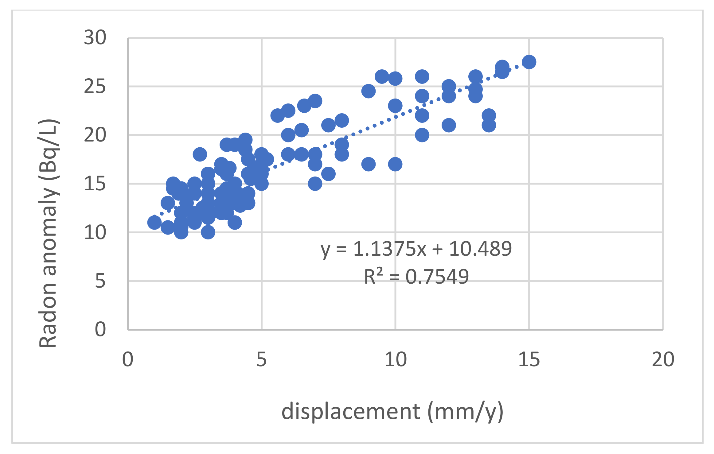
3.5. Relationship between Fault Activity and Radon Concentration

Thus far, many studies have been conducted on the relationship between the activity of faults and the increase in radon gas [45,47,48,51,68]. These studies show that the amount of radon in the air and dissolved in groundwater has always increased along with active faults. Increased stress due to the movement of fault blocks releases radon gas from adjacent rocks [49,50].

4. Results and Discussion

4.1. PSI Analysis

We applied the interferometry technique as a time series on 148 images. This study extracted 146 interferograms from the study area. The interferograms showed that the cumulative phase fluctuated between 0 and 2π. Using the PSI method on interferograms, we determined 1985 and 1920 persistent scatterer points for descending and ascending images in the northern range of the Anar fault. This study extracted 2450 and 2534 persistent scatterer points for descending and ascending images in the southern range of the Anar fault. Then, we calculated the displacement rate of these points. Figure 5a–d illustrates the location map of PSI points and their displacement rate related to the two-part Anar fault (see Figure 1). The results showed that the LOS displacement rate varied from +5 mm to −15 mm in both areas. The displacements occurred in the satellite look direction so that positive numbers indicate the proximity of the surface to the satellite and the uplift. The negative numbers indicate the distance of the surface from the satellite and subsidence. The red spots in the study area show subsidence of more than 15 mm per year. As shown in Figure 5c,d, there are two large subsidence zones on both sides of the Anar fault with an area of 80 km² and 16 km², respectively. Considering the subsidence issue in Iranian plains due to the groundwater discharge, we can estimate that the two indicated large subsidence zones are caused by the displacement [22,41].

We attempted further investigation to support the evidence of fault activity. This study observed two subsidence ranges (Figure 5) (see the rectangle on the map). Our results identified more subsidence on the Anar fault (i.e., N–S extent) generated by the seismic and fault activity. This study shows that the displacement rate occurring along the fault is less than the two subsidence areas’ displacement rates caused by irregular groundwater discharge. This study also measured the 3D displacement rate on the fault surface for the movement structure analysis of the Anar fault. We provide the results of the 3D displacement measurement in the following section.

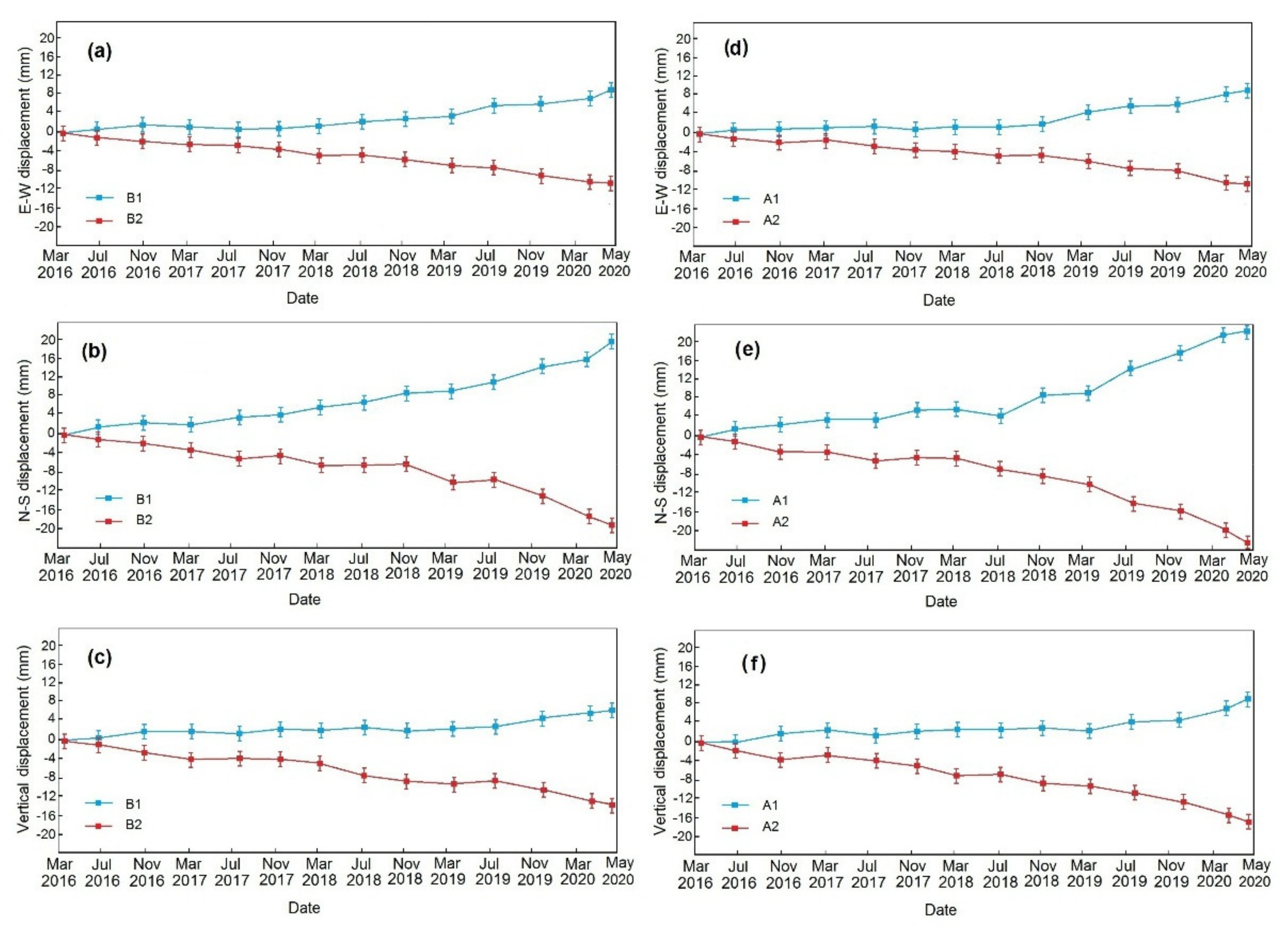
4.2. 3D Displacement Fields

As a result of the Sentinel satellite’s N–S orbit, only E–W and vertical displacement fields were extracted from the combined displacement maps of descending and ascending images. Meanwhile, there was still a need to combine three independent observations for preparing a 3D displacement field, including LOS and azimuth direction (derived from azimuth offset method) observations. We prepared a 3D displacement map in the fault range by combining the direction of azimuth and LOS observations (Figure 6). This study estimated that the E–W, N–S, and vertical component displacement rates are (2mm, −2mm), (5mm, −5mm), and (2mm, −3mm) per year, respectively. In the northern range of the Anar fault and (2mm, −2mm), (6mm, −6mm), and (2mm, −4mm) per year, respectively, and in the southern range of the Anar fault. Figure 6 shows that the fault line’s displacements and movements occurred on both sides. Therefore, these movements can be considered fault blocks. As we can see in Figure 6b, the N–S displacement component indicates the movement of the right block of the fault with the displacement rate of 6 mm per year to the south and the left block’s movement with the same displacement rate to the north. As shown in Figure 6c, the vertical displacement component represents the uplift and subsidence of fault blocks. The right and left blocks are uplifting and subsiding with the displacement rate of 4 mm and 2 mm per year, respectively. Finally, the E–W displacement component shows the displacement and receding of two fault blocks from each other at the rate of 2 mm per year. Therefore, by determining the 3D displacement field measurement, we can identify the Anar fault’s mechanism in the plain.

To investigate and monitor the movement behavior of fault blocks over time, we performed a time-series analysis on B1, B2, A1, and A2 points. Figure 7 illustrates the graphs of the fault activity mechanism analysis. As shown in the figure, point B1 and A1 are located on the fault’s right block and point B2 and A2 are located on the left block of the fault. In these graphs, we superimposed a 3D displacement rate on the vertical axis, and the duration of the study period was on the horizontal axis. As seen in this figure, the movements of the fault blocks were in opposite directions.

Additionally, in these graphs, the displacement graph’s slope in the last year of the study period increased in all displacement fields, especially in N–S displacement (Figure 6b,e). This increasing trend of displacement is due to the increased fault activity. As seen in Figure 6, the cumulative N–S displacement rate that occurred over four years reached approximately 24 mm, moving about 8 mm and 16 mm in the E–W and vertical directions, respectively.

4.3. PSI Validation

The Validation of the proposed approach and PSI analysis results was done based on the GPS observations precise measurements in the Anar city, which belongs to the National Cartographic Center (NCC) of Iran as the only GPS point station located in the study area. The GPS measurements of this point were carried out from 2018 to 2020 using Leica GX 1220 receiver. We presented the time series of deformation for the PS point (marked as “D” in Figure 8) and the GPS observations point (marked as “C” in Figure 8). However, the comparison of PSI results and GPS measurements on PS point C and GPS point D reveals that the cumulative displacement measurement from PSI agrees with the cumulative displacement measurement from GPS. The misfit between the leveling GPS results data and time series analysis results was expressed as RMSE, which estimated as 0.142 mm.

4.4. Anar Fault Tectonic Model

By observing the results of this study, we revealed that the Anar fault could be considered a right-lateral strike-slip fault with the normal component. To further investigate the movement mechanism of the Anar fault, we drew the 3D displacement profiles perpendicular to the fault line. The profiles are related to the persistent scatterer points and the a-b profile (shown in Figure 6). The 3D profiles show the Anar fault’s effect on the sudden Anar fault displacements. The points drawn on the maps are the same persistent scatterer points which are located based on the displacement rate and distance from the fault. This study shows that the dominant movement along the strike-slip fault is N–S and has the maximum displacement rates compared to the E–W and vertical movements. Compared to previous studies that recognized the Anar fault as a strike-slip fault [14,46,54], this study identifies that the Anar fault is a lateral strike-slip and oblique fault. Further evidence that can be used for the analysis of the Anar fault movement mechanism is the fall and descent of the ground surface between the two branches of the pomegranate fault (Figure 5a,b).

Shear folds are one of the structures that are created due to the lateral motion of the strike-slip faults. Field evidence showed that these folds in the Anar plain end adjacent to the fault (Figure 9a). In the southern part of the Anar fault, the fault trace with deviation in the path of the Qantas is clearly visible (Figure 9b). Due to the fault plane’s strike-slip movement, which dominates in the rock units and alluvial fans, the Qanat canals are excavated with a deviation close to the fault plane by pitmen (Figure 9c,d).

Therefore, according to the collected evidence, we can likely develop a tectonic model for the southern termination of the Anar fault system that looks like a flower structure forming a depressed area in the plain (Figure 10) [69]. Our data and the shape, nature, and general pattern of the Anar basin strongly suggest that the basin is an active negative flower structure.

4.5. Radon Analysis

Many studies imply a direct relationship between the activity of faults and the radon concentration in groundwater resources. This study investigated and monitored the fault activity for three years by measuring radon concentration in groundwater proximate to the Anar fault and its correlation with the fault. The results of measuring radon dissolved in the groundwater samples obtained from 40 wells over three years from 2018 to 2020 are shown in Table 2. Accordingly, in 2018, the highest radon concentration of 29.48 Bq/L was related to the water sample of 27 wells. This concentration reached 29.88 Bq/L and 31.73 Bq/L in the subsequent years. This increasing trend of radon concentration occurred in almost all wells.

Figure 11 illustrates the semivariogram surface maps of radon data and modelled experimental variograms used in the kriging algorithm to calculate anomaly maps. The parameters of the fitting models are used in the kriging algorithm calculations to predict (interpolate) “observation” values at unsampled locations within the area of interest. The prediction uses the spatial dependencies of the measurement values of the input data provided by the variograms.

As mentioned in the methodology section, we divided the study area into nine classes, from very high to low in groundwater radon concentration (Figure 12). Findings from radon anomaly show the extent of high radon anomaly areas along the Anar fault. This anomaly reconfirms the relationship between the activity of the Anar fault and increased radon dissolved in groundwater. We also observed that the radon concentration continuously increases as we move closer to the fault (Figure 12). In particular, in this study, the rising and expanding trend of areas with high radon anomalies overtime correctly shows a comparison of anomalous maps for 2018 to 2020.

4.6. Relationship between Radon Anomaly and Fault Displacement

To determine the relationships between the displacement of the earth’s surface, the amount of radon gas dissolved in groundwater, and the Anar fault, the profile of their changes along with the profile AB were drawn (Figure 13). As shown in Figure 13, both PSI displacement and radon concentration graphs have an upward trend as they approach the fault. In addition, to determine the correlation between the two variables of displacement rate and radon gas concentration, a scattergram was drawn. As shown in Figure 14, there is an acceptable correlation between them.

Finally, given the increasing displacement rate (calculated by the PSI method) adjacent to the Anar fault and the rising concentration of radon dissolved in the groundwater near the fault, all the cases mentioned above occurred as the result of increasing stress in the fault planes. This signature and evidence predicted the earthquake occurrence in the region.

5. Conclusions

Remote sensing techniques and Sentinel-1 images support monitoring the seismic activity and measuring the displacement of a fault. By monitoring the seismic activity movements, we observed the high progressive activity of the Anar fault. Results of the PSI method also led to our conclusion that the displacement rates at the ground surface are continuously increasing. The resulting analysis of 148 Sentinel-1 satellite images showed that the displacement and ground deformation is caused by continuous groundwater discharge and Anar fault activities. Therefore, we can determine that the displacement and subsidence rate in the study area depends on the groundwater discharge rate and Anar fault activities.

The 3D displacement components and profiles provided valuable information about the Anar fault mechanism. We could infer that the fault mechanism in the plain is the right-lateral strike-slip with the normal component. We determined the highest displacement rate of the N–S activity compared to other 3D displacement components. This displacement showed that the movements occur on both sides of the fault line. The time series analysis of points located on the fault blocks also confirmed the increase of the displacement rate of fault blocks. We also observed that the displacement of the Anar fault is a combination of oblique and lateral strike-slip movement. Therefore, based on the evidence, we determined that the tectonic mechanism of the fault formed the depressed area. This study suggests that the Anar basin is an active negative flower structure. Moreover, the three earthquakes have occurred within the following time intervals: 4.4 ± 0.8, 6.8 ± 1 and 9.8 ± 2 ka. The preferred age of the more recent event, ranging between 3600 and 5200 yr, suggested that the fault is approaching the end of its seismic cycle.

The radon concentration dissolved in the groundwater proximate to the monitored Anar fault provides evidence of the relationship between the fault activity and the increase in radon concentration in groundwater sources. The results showed higher radon concentration in the samples close to the fault along with its relative increase during the study period. According to the end of the return period of magnitude 7.0 earthquakes, and based on this study’s results, there is a high probability of a destructive earthquake in the near future. Therefore, in a future study, the authors are eager to collect data and develop an algorithm to learn the system for intelligent real-time fault displacement detection by combining InSAR, land surface temperature (LST), radon concentration anomaly, and recurrent neural networks. However, we suggest the importance of understanding the logical relationship between radon and PSI to determine and develop a fault activity prediction model.

References

1. Nicol, A.; Walsh, J.; Manzocchi, T.; Morewood, N. Displacement rates and average earthquake recurrence intervals on normal faults. J. Struct. Geol. 2005, 27, 541–551. [Google Scholar] [CrossRef]
2. Sertel, E.; Kaya, S.; Curran, P.J. Use of Semivariograms to Identify Earthquake Damage in an Urban Area. IEEE Trans. Geosci. Remote Sens. 2007, 45, 1590–1594. [Google Scholar] [CrossRef]
3. Mehrabi, A.; Dastanpour, M.; Radfar, S.; Vaziri, M.; Derakhshani, R. Detection of fault lineaments of the Zagros fold-thrust belt based on Landsat imagery interpretation and their relationship with Hormuz series salt dome locations using GIS analysis. Geosciences 2015, 24, 17–32. [Google Scholar] [CrossRef]
4. McClymont, A.F.; Villamor, P.; Green, A.G. Fault displacement accumulation and slip rate variability within the Taupo Rift (New Zealand) based on trench and 3-D ground-penetrating radar data. Tectonics 2009, 28, 28. [Google Scholar] [CrossRef]
5. Stramondo, S. The Tohoku–Oki Earthquake: A Summary of Scientific Outcomes from Remote Sensing. IEEE Geosci. Remote Sens. Lett. 2013, 10, 895–897. [Google Scholar] [CrossRef] [Green Version]
6. Hicks, S.P.; Rietbrock, A. Seismic slip on an upper-plate normal fault during a large subduction megathrust rupture. Nat. Geosci. 2015, 8, 955–960. [Google Scholar] [CrossRef] [Green Version]
7. Chen, Q.; Liu, X.; Zhang, Y.; Zhao, J.; Xu, Q.; Yang, Y.; Liu, G. A nonlinear inversion of InSAR-observed coseismic surface deformation for estimating variable fault dips in the 2008 Wenchuan earthquake. Int. J. Appl. Earth Obs. Geoinf. 2019, 76, 179–192. [Google Scholar] [CrossRef]
8. Vorobieva, I.; Ismail-Zadeh, A.; Gorshkov, A. Nonlinear dynamics of crustal blocks and faults and earthquake occurrences in the Transcaucasian region. Phys. Earth Planet. Inter. 2019, 297, 106320. [Google Scholar] [CrossRef]
9. Chin, T.-L.; Chen, K.-Y.; Chen, D.-Y.; Lin, D.-E. Intelligent Real-Time Earthquake Detection by Recurrent Neural Networks. IEEE Trans. Geosci. Remote Sens. 2020, 58, 5440–5449. [Google Scholar] [CrossRef]
10. Barnhart, W.D.; Gold, R.D.; Hollingsworth, J. Localized fault-zone dilatancy and surface inelasticity of the 2019 Ridgecrest earthquakes. Nat. Geosci. 2020, 13, 1–6. [Google Scholar] [CrossRef]
11. Derakhshani, R.; Eslami, S.S. A New Viewpoint for Seismotectonic Zoning. Am. J. Environ. Sci. 2011, 7, 212–218. [Google Scholar] [CrossRef]
12. Ali, S.; Pirasteh, S. Geological application of Landsat ETM for mapping structural geology and interpretation: Aided by remote sensing and GIS. Int. J. Remote Sens. 2004, 25, 4715–4727. [Google Scholar] [CrossRef]
13. Pirasteh, S.; Woodbridge, K.; Rizvi, S.M.A. Geo-information technology (GiT) and tectonic signatures: The River Karun & Dez, Zagros Orogen in south-west Iran. Int. J. Remote Sens. 2008, 30, 389–403. [Google Scholar] [CrossRef]
14. Foroutan, M.; Sébrier, M.; Nazari, H.; Meyer, B.; Fattahi, M.; Rashidi, A.; Dortz, K.L.; Bateman, M.D. New evidence for large earthquakes on the Central Iran plateau: Palaeoseismology of the Anar fault. Geophys. J. Int. 2012, 189, 6–18. [Google Scholar] [CrossRef] [Green Version]
15. Amato, V.; Aucelli, P.P.; Sessa, E.B.; Cesarano, M.; Incontri, P.; Pappone, G.; Valente, E.; Vilardo, G. Multidisciplinary approach for fault detection: Integration of PS-InSAR, geomorphological, stratigraphic and structural data in the Venafro intermontane basin (Central-Southern Apennines, Italy). Geomorphology 2017, 283, 80–101. [Google Scholar] [CrossRef]
16. Poreh, D.; Pirasteh, S. InSAR observations and analysis of the Medicina Geodetic Observatory and CosmoSkyMed images. Nat. Hazards 2020, 103, 1–17. [Google Scholar] [CrossRef]
17. Rahbar, R.; Bafti, S.; Derakhshani, R. INVESTIGATION OF THE TECTONIC ACTIVITY OF BAZARGAN MOUNTAIN IN IRAN. Sustain. Dev. Mt. Territ. 2017, 9, 380–386. [Google Scholar] [CrossRef]
18. Kermani, A.F.; Derakhshani, R.; Bafti, S.S. Data on morphotectonic indices of Dashtekhak district, Iran. Data Brief. 2017, 14, 782–788. [Google Scholar] [CrossRef]
19. Sousa, J.J.; Ruiz, A.M.; Hooper, A.J.; Hanssen, R.F.; Perski, Z.; Bastos, L.C.; Gil, A.J.; Galindo-Zaldívar, J.; De Galdeano, C.S.; Alfaro, P.; et al. Multi-temporal InSAR for Deformation Monitoring of the Granada and Padul Faults and the Surrounding Area (Betic Cordillera, Southern Spain). Procedia Technol. 2014, 16, 886–896. [Google Scholar] [CrossRef] [Green Version]
20. Zhang, Y.; Liu, C.; Zhang, W.; Jiang, F. Present-Day Deformation of the Gyaring Co Fault Zone, Central Qinghai–Tibet Plateau, Determined Using Synthetic Aperture Radar Interferometry. Remote Sens. 2019, 11, 1118. [Google Scholar] [CrossRef] [Green Version]
21. Hung, W.-C.; Hwang, C.; Chen, Y.-A.; Chang, C.-P.; Yen, J.-Y.; Hooper, A.; Yang, C.-Y. Surface deformation from persistent scatterers SAR interferometry and fusion with leveling data: A case study over the Choushui River Alluvial Fan, Taiwan. Remote Sens. Environ. 2011, 115, 957–967. [Google Scholar] [CrossRef]
22. Ghazifard, A.; Moslehi, A.; Safaei, H.; Roostaei, M. Effects of groundwater withdrawal on land subsidence in Kashan Plain, Iran. Bull. Int. Assoc. Eng. Geol. 2016, 75, 1157–1168. [Google Scholar] [CrossRef]
23. Guo, J.; Xu, S.; Fan, H. Neotectonic interpretations and PS-InSAR monitoring of crustal deformations in the Fujian area of China. Open Geosci. 2017, 9, 126–132. [Google Scholar] [CrossRef]
24. Gong, W.; Zhang, Y.; Li, T.; Wen, S.; Zhao, D.; Hou, L.; Shan, X. Multi-Sensor Geodetic Observations and Modeling of the 2017 Mw 6.3 Jinghe Earthquake. Remote Sens. 2019, 11, 2157. [Google Scholar] [CrossRef] [Green Version]
25. Kuna, V.M.; Nábělek, J.L.; Braunmiller, J. Mode of slip and crust–mantle interaction at oceanic transform faults. Nat. Geosci. 2019, 12, 138–142. [Google Scholar] [CrossRef]
26. Mehrabi, A. Monitoring the Iran Pol-e-Dokhtar flood extent and detecting its induced ground displacement using sentinel 1 imagery techniques. Nat. Hazards 2021, 105, 2603–2617. [Google Scholar] [CrossRef]
27. Ghayournajarkar, N.; Fukushima, Y. Determination of the dipping direction of a blind reverse fault from InSAR: Case study on the 2017 Sefid Sang earthquake, northeastern Iran. Earth Planets Space 2020, 72, 1–15. [Google Scholar] [CrossRef]
28. Song, X.; Jiang, Y.; Shan, X.; Qu, C. Deriving 3D coseismic deformation field by combining GPS and InSAR data based on the elastic dislocation model. Int. J. Appl. Earth Obs. Geoinf. 2017, 57, 104–112. [Google Scholar] [CrossRef]
29. Qu, F.; Lu, Z.; Kim, J.-W.; Zheng, W. Identify and Monitor Growth Faulting Using InSAR over Northern Greater Houston, Texas, USA. Remote Sens. 2019, 11, 1498. [Google Scholar] [CrossRef] [Green Version]
30. Su, Z.; Yang, Y.-H.; Li, Y.-S.; Xu, X.-W.; Zhang, J.; Zhou, X.; Ren, J.-J.; Wang, E.-C.; Hu, J.-C.; Zhang, S.-M.; et al. Coseismic displacement of the 5 April 2017 Mashhad earthquake (Mw 6.1) in NE Iran through Sentinel-1A TOPS data: New implications for the strain partitioning in the southern Binalud Mountains. J. Asian Earth Sci. 2019, 169, 244–256. [Google Scholar] [CrossRef]
31. Sansosti, E.; Berardino, P.; Bonano, M.; Calò, F.; Castaldo, R.; Casu, F.; Manunta, M.; Manzo, M.; Pepe, A.; Pepe, S.; et al. How second generation SAR systems are impacting the analysis of ground deformation. Int. J. Appl. Earth Obs. Geoinf. 2014, 28, 1–11. [Google Scholar] [CrossRef] [Green Version]
32. Wang, X.; Liu, G.; Yu, B.; Dai, K.; Zhang, R.; Ma, D.; Li, Z. An integrated method based on DInSAR, MAI and displacement gradient tensor for mapping the 3D coseismic deformation field related to the 2011 Tarlay earthquake (Myanmar). Remote Sens. Environ. 2015, 170, 388–404. [Google Scholar] [CrossRef]
33. Ran, Y.; Xu, X.; Wang, H.; Chen, W.; Chen, L.; Liang, M.; Yang, H.; Li, Y.; Liu, H. Evidence of Characteristic Earthquakes on Thrust Faults from Paleo-Rupture Behavior Along the Longmenshan Fault System. Tectonics 2019, 38, 2401–2410. [Google Scholar] [CrossRef]
34. Luo, H.; Wang, K. Postseismic geodetic signature of cold forearc mantle in subduction zones. Nat. Geosci. 2021, 14, 104–109. [Google Scholar] [CrossRef]
35. Mouslopoulou, V.; Walsh, J.J.; Nicol, A. Fault displacement rates on a range of timescales. Earth Planet. Sci. Lett. 2009, 278, 186–197. [Google Scholar] [CrossRef]
36. Wu, C.; Zheng, W.; Zhang, Z.; Jia, Q.; Yang, H. Large-earthquake rupturing and slipping behavior along the range-front Maidan fault in the southern Tian Shan, northwestern China. J. Asian Earth Sci. 2020, 190, 104193. [Google Scholar] [CrossRef]
37. Stemberk, J.; Moro, G.D.; Stemberk, J.; Blahůt, J.; Coubal, M.; Košťák, B.; Zambrano, M.; Tondi, E. Strain monitoring of active faults in the central Apennines (Italy) during the period 2002–2017. Tectonophysics 2019, 750, 22–35. [Google Scholar] [CrossRef]
38. Hooper, A. A multi-temporal InSAR method incorporating both persistent scatterer and small baseline approaches. Geophys. Res. Lett. 2008, 35. [Google Scholar] [CrossRef] [Green Version]
39. Yaseen, M.; Hamm, N.; Woldai, T.; Tolpekin, V.; Stein, A. Local interpolation of coseismic displacements measured by InSAR. Int. J. Appl. Earth Obs. Geoinf. 2013, 23, 1–17. [Google Scholar] [CrossRef]
40. Ferretti, A.; Fumagalli, A.; Novali, F.; Prati, C.; Rocca, F.; Rucci, A. A New Algorithm for Processing Interferometric Data-Stacks: SqueeSAR. IEEE Trans. Geosci. Remote Sens. 2011, 49, 3460–3470. [Google Scholar] [CrossRef]
41. Liu, G.; Li, J.; Xu, Z.; Wu, J.; Chen, Q.; Zhang, H.; Zhang, R.; Jia, H.; Luo, X. Surface deformation associated with the 2008 Ms8.0 Wenchuan earthquake from ALOS L-band SAR interferometry. Int. J. Appl. Earth Obs. Geoinf. 2010, 12, 496–505. [Google Scholar] [CrossRef]
42. Berardino, P.; Fornaro, G.; Lanari, R.; Sansosti, E. A new algorithm for surface deformation monitoring based on small baseline differential SAR interferograms. IEEE Trans. Geosci. Remote Sens. 2002, 40, 2375–2383. [Google Scholar] [CrossRef] [Green Version]
43. Lanari, R.; Mora, O.; Manunta, M.; Mallorqui, J.; Berardino, P.; Sansosti, E. A small-baseline approach for investigating deformations on full-resolution differential SAR interferograms. IEEE Trans. Geosci. Remote Sens. 2004, 42, 1377–1386. [Google Scholar] [CrossRef]
44. Perissin, D.; Wang, T. Repeat-Pass SAR Interferometry with Partially Coherent Targets. IEEE Trans. Geosci. Remote Sens. 2011, 50, 271–280. [Google Scholar] [CrossRef]
45. Yalım, H.A.; Sandıkcıoğlu, A.; Ertuğrul, O.; Yıldız, A.; Yildiz, A. Determination of the relationship between radon anomalies and earthquakes in well waters on the Akşehir-Simav Fault System in Afyonkarahisar province, Turkey. J. Environ. Radioact. 2012, 110, 7–12. [Google Scholar] [CrossRef]
46. Yamani, M.; Goorabi, A.; Kakroodia, A. Evidence of Neotectonics along Dehshir and Anar Faults in Central Iran by Using Remote Sensing Data. Wulfenia 2013, 20, 1–29. [Google Scholar]
47. Amani, A.; Mansor, S.; Pradhan, B.; Billa, L.; Pirasteh, S. Coupling effect of ozone column and atmospheric infrared sounder data reveal evidence of earthquake precursor phenomena of Bam earthquake, Iran. Arab. J. Geosci. 2013, 7, 1517–1527. [Google Scholar] [CrossRef]
48. Ye, Q.; Singh, R.P.; He, A.; Ji, S.; Liu, C. Characteristic behavior of water radon associated with Wenchuan and Lushan earthquakes along Longmenshan fault. Radiat. Meas. 2015, 76, 44–53. [Google Scholar] [CrossRef]
49. Kawabata, K.; Sato, T.; Takahashi, H.A.; Tsunomori, F.; Hosono, T.; Takahashi, M.; Kitamura, Y. Changes in groundwater radon concentrations caused by the 2016 Kumamoto earthquake. J. Hydrol. 2020, 584, 124712. [Google Scholar] [CrossRef]
50. Tsunomori, F.; Shimodate, T.; Ide, T.; Tanaka, H. Radon concentration distributions in shallow and deep groundwater around the Tachikawa fault zone. J. Environ. Radioact. 2017, 172, 106–112. [Google Scholar] [CrossRef]
51. Seminsky, K.; Seminsky, A. Radon concentration in groundwater sources of the Baikal region (East Siberia, Russia). Appl. Geochem. 2019, 111, 104446. [Google Scholar] [CrossRef]
52. Zafar, W.A.; Ahmed, J.; Barkat, A.; Nabi, A.; Mahmood, R.; Manzoor, S.; Iqbal, T. Spatial mapping of radon: Implication for fault delineation. Geochem. J. 2018, 52, 359–371. [Google Scholar] [CrossRef] [Green Version]
53. Mehrabi, A.; Khabazi, M.; Almodaresi, A.; Nohesara, M.; Derakhshani, R. Land use changes monitoring over 30 years and prediction of future changes using multi-temporal Landsat imagery and the land change modeler tools in Rafsanjan city (Iran). Sustain. Dev. Mt. Territ. 2019, 11, 26–35. [Google Scholar] [CrossRef]
54. Dortz, K.L.; Meyer, B.; Sébrier, M.; Nazari, H.; Braucher, R.; Fattahi, M.; Benedetti, L.; Foroutan, M.; Siame, L.; Bourlès, D.; et al. Holocene right-slip rate determined by cosmogenic and OSL dating on the Anar fault, Central Iran. Geophys. J. Int. 2009, 179, 700–710. [Google Scholar] [CrossRef] [Green Version]
55. Woodbridge, K.P.; Pirasteh, S.; Parsons, D.R. Investigating Fold-River Interactions for Major Rivers Using a Scheme of Remotely Sensed Characteristics of River and Fold Geomorphology. Remote Sens. 2019, 11, 2037. [Google Scholar] [CrossRef] [Green Version]
56. Ali, S.A.; Rangzan, K.; Pirasteh, S. Remote Sensing and GIS Study of Tectonics and Net Erosion Rates in the Zagros Structural Belt, Southwestern Iran. Mapp. Sci. Remote Sens. 2003, 40, 258–267. [Google Scholar] [CrossRef]
57. Mehrabi, A.; Derakhshani, R. Generation of integrated geochemical-geological predictive model of porphyry-Cu potential, Chahargonbad District, Iran. Geochim. Cosmochim. Acta 2010, 74, A649–A743. [Google Scholar] [CrossRef] [Green Version]
58. Derakhshani, R.; Mehrabi, A. Derakhshan Geologically-Constrained Fuzzy Mapping of Porphyry Copper Mineralization Potential, Meiduk District, Iran. Trends Appl. Sci. Res. 2009, 4, 229–240. [Google Scholar] [CrossRef]
59. Derakhshani, R.; Mehrabi, A. Spatial Association of Copper Mineralization and Faults/Fractures in Southern Part of Central Iranian Volcanic Belt. Trends Appl. Sci. Res. 2009, 4, 138–147. [Google Scholar] [CrossRef] [Green Version]
60. Agard, P.; Monié, P.; Gerber, W.; Omrani, J.; Molinaro, M.; Meyer, B.; Labrousse, L.; Vrielynck, B.; Jolivet, L.; Yamato, P. Transient, synobduction exhumation of Zagros blueschists inferred from P-T, deformation, time, and kinematic constraints: Implications for Neotethyan wedge dynamics. J. Geophys. Res. Space Phys. 2006, 111. [Google Scholar] [CrossRef]
61. Berberian, M.; Jackson, J.; Fielding, E.J.; Parsons, B.; Priestley, K.F.; Qorashi, M.; Talebian, M.; Walker, R.; Wright, T.J.; Baker, C.V.H. The 1998 March 14 Fandoqa earthquake (Mw6.6) in Kerman province, southeast Iran: Re-rupture of the 1981 Sirch earthquake fault, triggering of slip on adjacent thrusts and the active tectonics of the Gowk fault zone. Geophys. J. Int. 2001, 146, 371–398. [Google Scholar] [CrossRef] [Green Version]
62. Rashidi Boshrabadi, A.; Khatib, M.M.; Raeesi, M.; Mousavi, S.M.; Djamour, Y.; Rashidi, A.; Jamour, Y. Geometric-kinematic characteristics of the main faults in the W-SW of the Lut Block (SE Iran). J. Afr. Earth Sci. 2018, 139, 440–462. [Google Scholar] [CrossRef]
63. Hessami, K.; Nilforoushan, F.; Talbot, C. Active deformation within the Zagros Mountains deduced from GPS measurements. J. Geol. Soc. 2006, 163, 143–148. [Google Scholar] [CrossRef] [Green Version]
64. Pirasteh, S.; Safari, H.O.; Mollaee, S. Digital Processing of SAR Data and Image Analysis Techniques. In Monitoring and Modeling of Global Changes: A Geomatics Perspective; Springer: Berlin/Heidelberg, Germany, 2015; pp. 281–299. [Google Scholar]
65. Michel, R.; Avouac, J.-P.; Taboury, J. Measuring ground displacements from SAR amplitude images: Application to the Landers Earthquake. Geophys. Res. Lett. 1999, 26, 875–878. [Google Scholar] [CrossRef] [Green Version]
66. Fattahi, H.; Agram, P.; Simons, M. A Network-Based Enhanced Spectral Diversity Approach for TOPS Time-Series Analysis. IEEE Trans. Geosci. Remote Sens. 2017, 55, 777–786. [Google Scholar] [CrossRef] [Green Version]
67. Wegnüller, U.; Werner, C.; Strozzi, T.; Wiesmann, A.; Frey, O.; Santoro, M. Sentinel-1 Support in the GAMMA Software. Procedia Comput. Sci. 2016, 100, 1305–1312. [Google Scholar] [CrossRef] [Green Version]
68. Papastefanou, C. Variation of radon flux along active fault zones in association with earthquake occurrence. Radiat. Meas. 2010, 45, 943–951. [Google Scholar] [CrossRef]
69. Rashidi, A.; Abbassi, M.-R.; Nilfouroushan, F.; Shafiei, S.; Derakhshani, R.; Nemati, M. Morphotectonic and earthquake data analysis of interactional faults in Sabzevaran Area, SE Iran. J. Struct. Geol. 2020, 139, 104147. [Google Scholar] [CrossRef]
Figure 1. The study area and Anar fault in the Central Iran block (UTM Zone 40).
Remotesensing 13 02072 g001
Figure 2. (a) The Anar fault trace in the south termination. (b) Field image of the Anar fault scarp. (c) Topographic cross-section perpendicular to the fault, which shows ~30 m of the scarp. (d,e) Two scenarios that could have created the Anar fault scarp.
Remotesensing 13 02072 g002
Figure 3. Flowchart of the research method.
Remotesensing 13 02072 g003
Figure 4. Connection graph between the master (red dot) and slave (black dots) images generated with the PSI method. Graphs were obtained from (a) the descending and (b) the ascending Sentinel-1 dataset.
Remotesensing 13 02072 g004
Figure 5. The LOS displacement map from the PSI method. (a,c) ascending images; (b,d) descending images. A dark line marks the Anar fault. The rectangles indicate the areas where the azimuth offset method is applied.
Remotesensing 13 02072 g005
Figure 6. Mechanism of the displacement component (E–W, N–S, and vertical) for the Anar fault activity. Combination of oblique and lateral strike-slip fault. Velocity component and displacement profiles (a,d) E–W, (b,e) N–S, and (c,f) vertical.
Remotesensing 13 02072 g006
Figure 7. Time series graph of the displacement of fault blocks at points A1, A2 and B1, B2; the position of points A1, A2 and B1, B2 (see Figure 6). (a,d) E–W displacement, (b,e) N–S displacement, (c,f) vertical displacement.
Remotesensing 13 02072 g007
Figure 8. (a) Displacement measurement, (b) comparison between PSI results vs. GPS measurements on PS point C and GPS point D shown in (a).
Remotesensing 13 02072 g008
Figure 9. (a) Shear folding along the Anar fault zone. (b) The trace of the southern part of the Anar fault. (c,d) The deflection of the qanat at the closing of the fault trace.
Remotesensing 13 02072 g009
Figure 10. Block diagram illustrating the structural evolution of the southern termination of the Anar fault.
Remotesensing 13 02072 g010
Figure 11. Semivariogram surface maps of radon data and modelled experimental variograms were calculated for data collected in the study area (a) related to 2017–2018 data; (b) related to 2018–2019 data; (c) related to 2019–2020 data.
Remotesensing 13 02072 g011
Figure 12. Classified map of radon anomaly in the study area: (a) 2018, (b) 2019, and (c) 2020. Bottom right figure shows radon anomaly profile AB, CD, and EF.
Remotesensing 13 02072 g012
Figure 13. Displacement rate and radon anomaly cross-section profiles highlight a good correlation of Rn and displacement rate peaks with the fault trace.
Remotesensing 13 02072 g013
Figure 14. Scattergram for the relationship between the displacement rate and radon gas concentration at the same measurement points.
Remotesensing 13 02072 g014