
Combining Regional Habitat Selection Models for Large-Scale Prediction: Circumpolar Habitat Selection of Southern Ocean Humpback Whales

 , , ,
, , ,  and
and
Abstract
:
1. Introduction
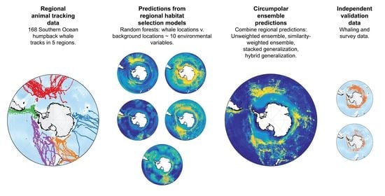
2. Methods
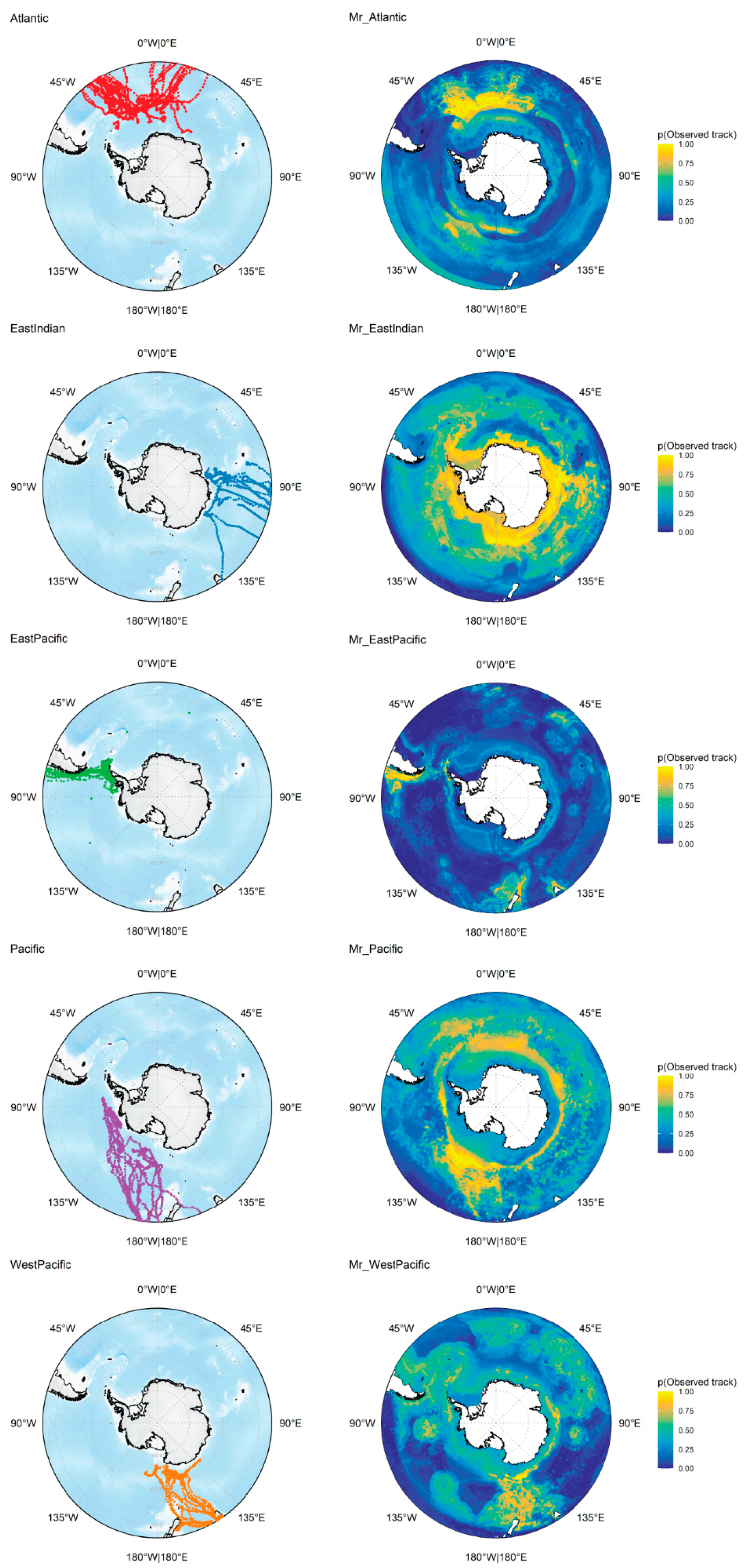
2.1. Whale Tracking Data
2.2. Estimating Whale Habitat Availability
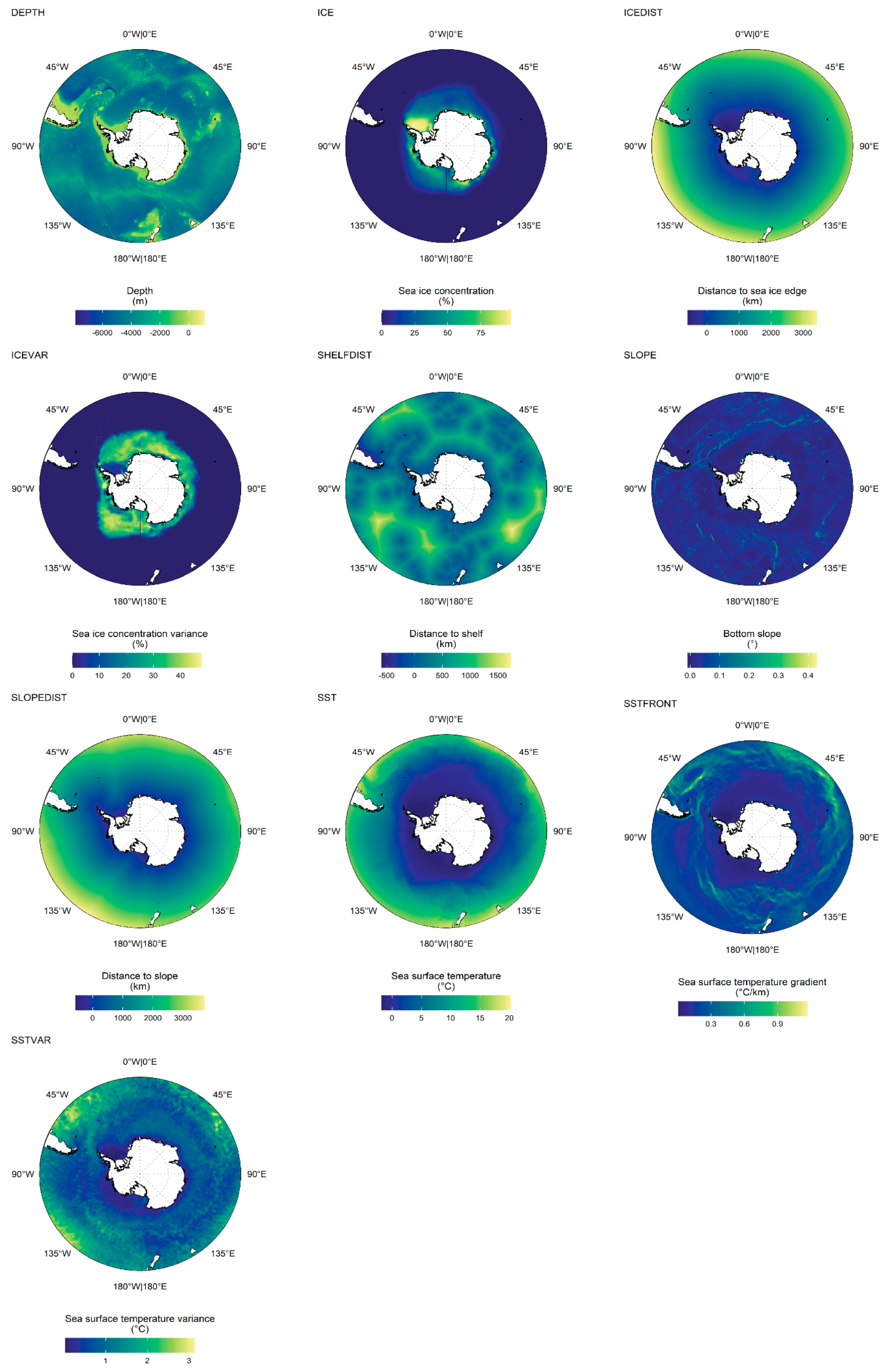
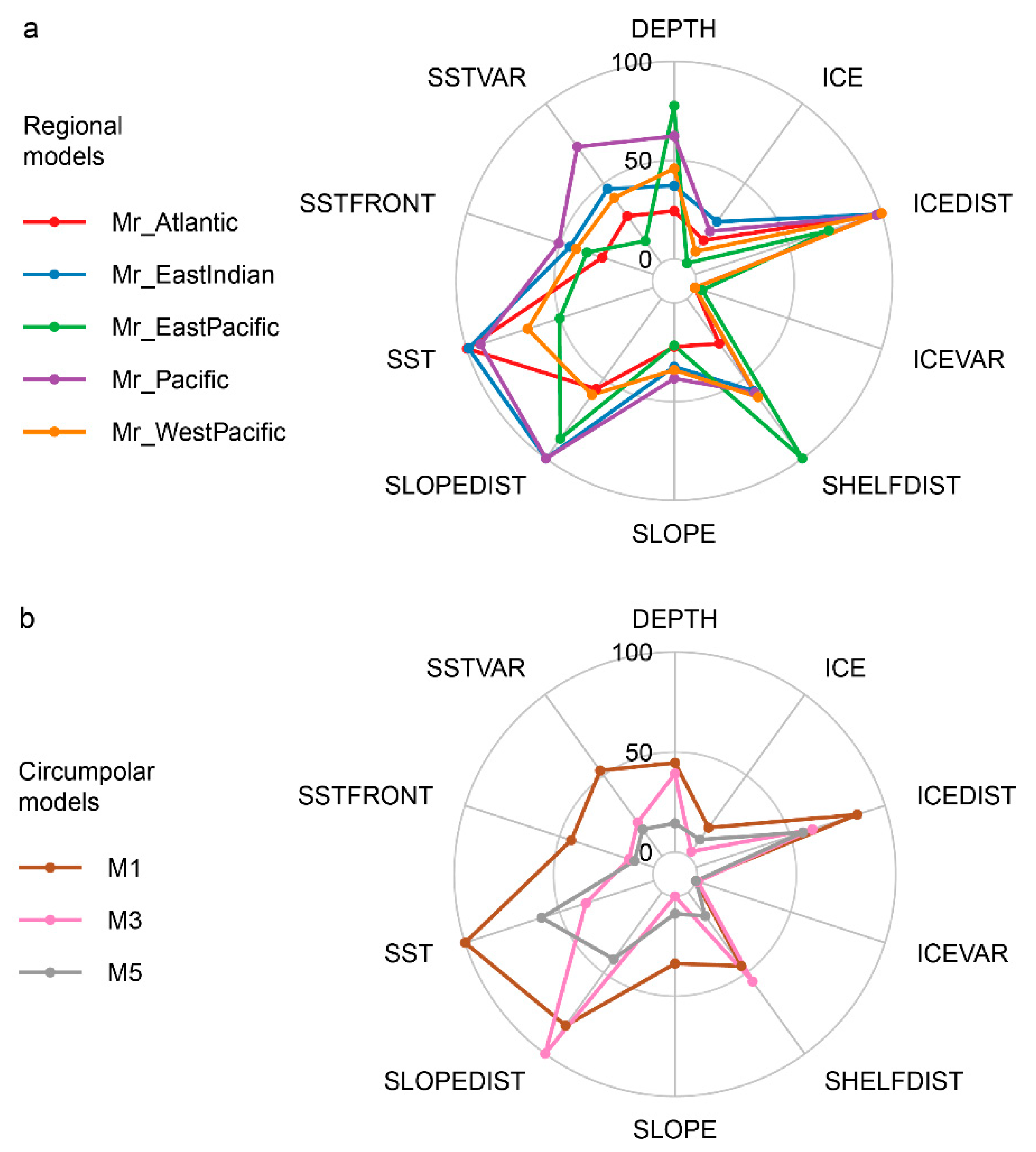
2.3. Environmental Covariates
2.4. Modelling Approaches
2.4.1. M1—A Naive Circumpolar Model
2.4.2. Mr—Regional Models
2.4.3. M2—Unweighted Ensemble (Simple Averaging)
2.4.4. M3—Similarity-Weighted Ensemble
2.4.5. M4—Stacked Generalization
2.4.6. M5—Hybrid Generalization
2.5. Model Fitting
2.6. Extrapolation
2.7. Independent Validation Data
3. Results
3.1. Regional Models
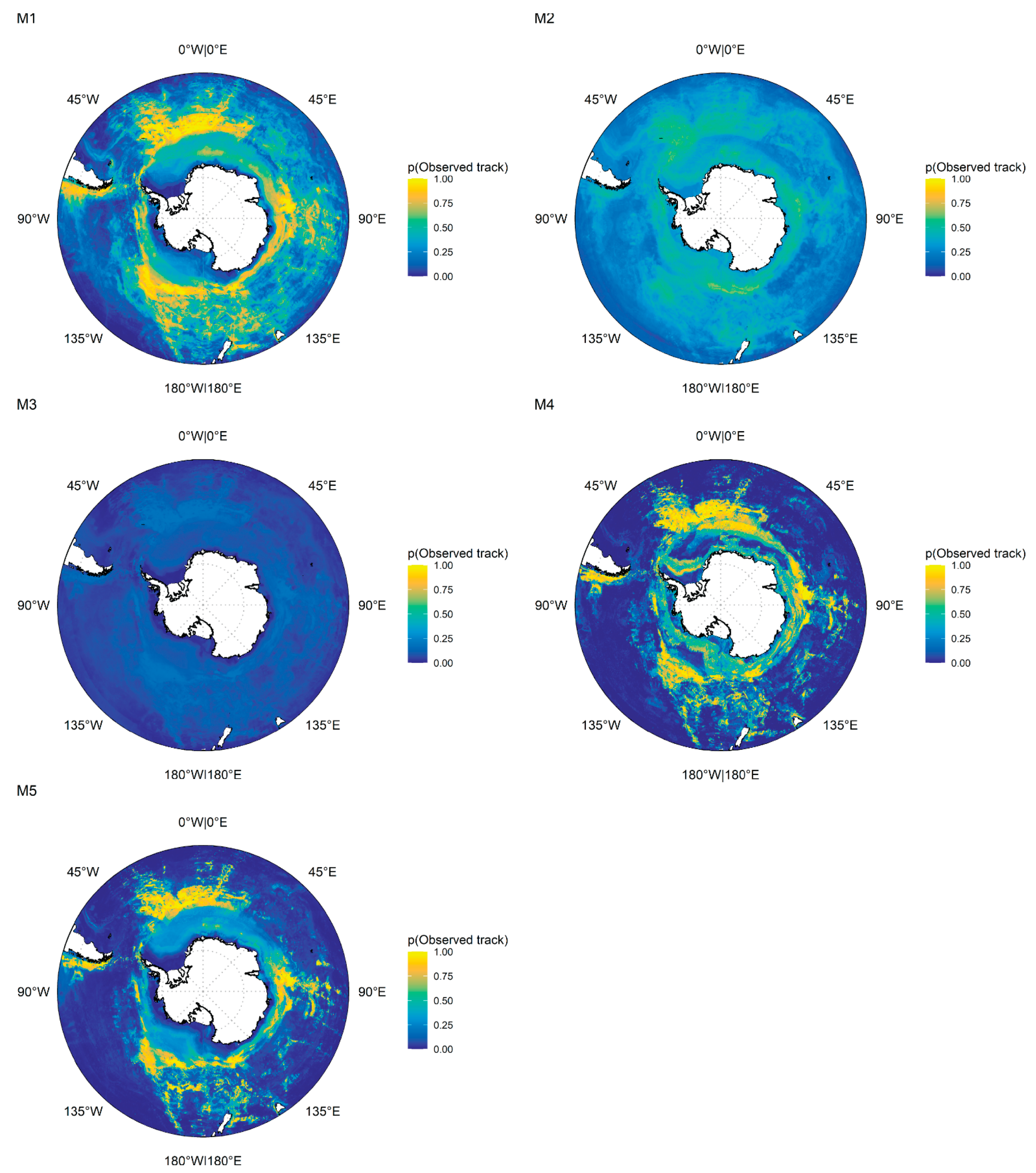
3.2. Circumpolar Models
4. Discussion
Humpback Whale Circumpolar Habitat Selection Patterns
5. Conclusions
Supplementary Materials
Author Contributions
Funding
Institutional Review Board Statement
Informed Consent Statement
Data Availability Statement
Acknowledgments
Conflicts of Interest
References
- Boyce, M.S.; McDonald, L.L. Relating populations to habitats using resource selection functions. Trends Ecol. Evol. 1999, 14, 268–272. [Google Scholar] [CrossRef]
- Manly, B.F.J.; McDonald, L.L.; Thomas, D.L.; McDonald, T.L.; Erickson, W.P. Resource Selection by Animals: Statistical Design and Analysis for Field Studies; Kluwer Academic Publishers: Dordrecht, The Netherlands, 2004. [Google Scholar] [CrossRef]
- Elith, J.; Leathwick, J.R. Species Distribution Models: Ecological Explanation and Prediction across Space and Time. Annu. Rev. Ecol. Evol. Syst. 2009, 40, 677–697. [Google Scholar] [CrossRef]
- Gregr, E.; Baumgartner, M.; Laidre, K.; Palacios, D. Marine mammal habitat models come of age: The emergence of ecological and management relevance. Endanger. Species Res. 2013, 22, 205–212. [Google Scholar] [CrossRef]
- Guisan, A.; Thuiller, W.; Zimmermann, N.E. Habitat Suitability and Distribution Models; Cambridge University Press: Cambridge, UK, 2017. [Google Scholar] [CrossRef]
- Humphries, G.; Magness, D.; Huettmann, F. Machine Learning for Ecology and Sustainable Natural Resource Management; Humphries, G., Magness, D.R., Huettmann, F., Eds.; Springer International Publishing: Cham, Switzerland, 2018. [Google Scholar] [CrossRef]
- Shoemaker, K.T.; Heffelfinger, L.; Jackson, N.J.; Blum, M.E.; Wasley, T.; Stewart, K.M. A machine-learning approach for extending classical wildlife resource selection analyses. Ecol. Evol. 2018, 8, 3556–3569. [Google Scholar] [CrossRef] [PubMed]
- Torres, L.G.; Sutton, P.J.H.; Thompson, D.R.; Delord, K.; Weimerskirch, H.; Sagar, P.M.; Phillips, R.A. Poor transferability of species distribution models for a pelagic predator, the grey petrel, indicates contrasting habitat preferences across ocean basins. PLoS ONE 2015, 10, e0120014. [Google Scholar] [CrossRef] [PubMed] [Green Version]
- Redfern, J.V.; Moore, T.J.; Fiedler, P.C.; de Vos, A.; Brownell, R.L.; Forney, K.A.; Ballance, L.T. Predicting cetacean distributions in data-poor marine ecosystems. Divers. Distrib. 2017, 23, 394–408. [Google Scholar] [CrossRef]
- Byrne, M.E.; Vaudo, J.J.; Harvey, G.C.M.; Johnston, M.W.; Wetherbee, B.M.; Shivji, M. Behavioral response of a mobile marine predator to environmental variables differs across ecoregions. Ecography 2019, 42, 1569–1578. [Google Scholar] [CrossRef]
- Mannocci, L.; Roberts, J.J.; Pedersen, E.J.; Halpin, P.N. Geographical differences in habitat relationships of cetaceans across an ocean basin. Ecography 2020, 43, 1250–1259. [Google Scholar] [CrossRef]
- Mysterud, A.; Ims, R.A. Functional responses in habitat use: Availability influences relative use in trade-off situations. Ecology 1998, 79, 1435–1441. [Google Scholar] [CrossRef]
- Holbrook, J.D.; Olson, L.E.; DeCesare, N.J.; Hebblewhite, M.; Squires, J.R.; Steenweg, R. Functional responses in habitat selection: Clarifying hypotheses and interpretations. Ecol. Appl. 2019, 29, e01852. [Google Scholar] [CrossRef]
- Van Beest, F.M.; McLoughlin, P.D.; Vander Wal, E.; Brook, R.K. Density-dependent habitat selection and partitioning between two sympatric ungulates. Oecologia 2014, 175, 1155–1165. [Google Scholar] [CrossRef] [PubMed]
- Matthiopoulos, J.; Fieberg, J.; Aarts, G.A.; Beyer, H.L.; Morales, J.M.; Haydon, D.T. Establishing the link between habitat selection and animal population dynamics. Ecol. Monogr. 2015, 85, 413–436. [Google Scholar] [CrossRef]
- Peterson, A.T.; Holt, R.D. Niche differentiation in Mexican birds: Using point occurrences to detect ecological innovation. Ecol. Lett. 2003, 6, 774–782. [Google Scholar] [CrossRef] [Green Version]
- Aarts, G.; MacKenzie, M.L.; McConnell, B.J.; Fedak, M.; Matthiopoulos, J. Estimating space-use and habitat preference from wildlife telemetry data. Ecography 2008, 31, 140–160. [Google Scholar] [CrossRef]
- Matthiopoulos, J.; Hebblewhite, M.; Aarts, G.; Fieberg, J. Generalized functional responses for species distributions. Ecology 2011, 92, 583–589. [Google Scholar] [CrossRef] [PubMed]
- Raymond, B.; Lea, M.-A.; Patterson, T.A.; Andrews-Goff, V.; Sharples, R.; Charrassin, J.-B.; Cottin, M.; Emmerson, L.; Gales, N.; Gales, R.; et al. Important marine habitat off east Antarctica revealed by two decades of multi-species predator tracking. Ecography 2014, 38, 121–129. [Google Scholar] [CrossRef]
- Araújo, M.B.; New, M. Ensemble forecasting of species distributions. Trends Ecol. Evol. 2007, 22, 42–47. [Google Scholar] [CrossRef]
- Zhou, Z.-H. Ensemble Methods: Foundations and Algorithms; CRC Press: Boca Raton, FL, USA, 2012. [Google Scholar]
- Brown, G. Ensemble Learning. In Encyclopedia of Machine Learning and Data Science, 2nd ed.; Sammut, C., Webb, G.I., Eds.; Springer: New York, NY, USA, 2017; pp. 393–402. [Google Scholar] [CrossRef]
- Kuncheva, L.I. Combining Pattern Classifiers: Methods and Algorithms, 2nd ed.; John Wiley & Sons, Ltd.: Hoboken, NJ, USA, 2014. [Google Scholar]
- Abrahms, B.; Welch, H.; Brodie, S.; Jacox, M.G.; Becker, E.A.; Bograd, S.J.; Irvine, L.M.; Palacios, D.M.; Mate, B.R.; Hazen, E.L. Dynamic ensemble models to predict distributions and anthropogenic risk exposure for highly mobile species. Divers. Distrib. 2019, 25, 1182–1193. [Google Scholar] [CrossRef] [Green Version]
- Scales, K.L.; Miller, P.I.; Ingram, S.N.; Hazen, E.L.; Bograd, S.J.; Phillips, R.A. Identifying predictable foraging habitats for a wide-ranging marine predator using ensemble ecological niche models. Divers. Distrib. 2015, 22, 212–224. [Google Scholar] [CrossRef] [Green Version]
- Reisinger, R.R.; Raymond, B.; Hindell, M.A.; Bester, M.N.; Crawford, R.J.M.; Davies, D.; De Bruyn, P.J.N.; Dilley, B.J.; Kirkman, S.P.; Makhado, A.B.; et al. Habitat modelling of tracking data from multiple marine predators identifies important areas in the Southern Indian Ocean. Divers. Distrib. 2018, 24, 535–550. [Google Scholar] [CrossRef] [Green Version]
- Hindell, M.A.; Reisinger, R.R.; Ropert-Coudert, Y.; Hückstädt, L.A.; Trathan, P.N.; Bornemann, H.; Charrassin, J.-B.; Chown, S.L.; Costa, D.P.; Danis, B.; et al. Tracking of marine predators to protect Southern Ocean ecosystems. Nature 2020, 580, 87–92. [Google Scholar] [CrossRef] [PubMed] [Green Version]
- Péron, C.; Authier, M.; Grémillet, D. Testing the transferability of track-based habitat models for sound marine spatial planning. Divers. Distrib. 2018, 24, 1772–1787. [Google Scholar] [CrossRef]
- Clapham, P.J.; Mead, J.G. Megaptera novaeangliae. Mamm. Species 1999, 40, 1–9. [Google Scholar] [CrossRef] [Green Version]
- International Whaling Commission. Report of the Scientific Committee. Annex H Report of the Sub-Committee on Other Southern Hemisphere Whale Stocks. J. Cetacean Res. Manag. 2016, 17, 250–282. [Google Scholar]
- Zerbini, A.N.; Andriolo, A.; Heide-Jorgensen, M.P.; Moreira, S.C.; Pizzorno, J.L.; Maia, Y.G.; Demaster, D.P. Migration and summer destinations of humpback whales (Megaptera novaeangliae) in the western South Atlantic Ocean. J. Cetacean Res. Manag. Spec. Issue 2011, 13, 113–118. [Google Scholar] [CrossRef]
- Zerbini, A.N.; Andriolo, A.; Heide-Jørgensen, M.; Pizzorno, J.; Maia, Y.; VanBlaricom, G.; Bethlem, C. Satellite-monitored movements of humpback whales Megaptera novaeangliae in the Southwest Atlantic Ocean. Mar. Ecol. Prog. Ser. 2006, 313, 295–304. [Google Scholar] [CrossRef] [Green Version]
- Dalla Rosa, L.; Secchi, E.R.; Maia, Y.G.; Zerbini, A.N.; Heide-Jørgensen, M.P. Movements of satellite-monitored humpback whales on their feeding ground along the Antarctic Peninsula. Polar Biol. 2008, 31, 771–781. [Google Scholar] [CrossRef]
- Rosenbaum, H.C.; Maxwell, S.M.; Kershaw, F.; Mate, B. Long-Range Movement of Humpback Whales and Their Overlap with Anthropogenic Activity in the South Atlantic Ocean. Conserv. Biol. 2014, 28, 604–615. [Google Scholar] [CrossRef]
- Curtice, C.; Johnston, D.W.; Ducklow, H.W.; Gales, N.J.; Halpin, P.N.; Friedlaender, A.S. Modeling the spatial and temporal dynamics of foraging movements of humpback whales (Megaptera novaeangliae) in the Western Antarctic Peninsula. Movement Ecol. 2015, 3, 1–9. [Google Scholar] [CrossRef] [Green Version]
- Garrigue, C.; Clapham, P.J.; Geyer, Y.; Kennedy, A.S.; Zerbini, A.N. Satellite tracking reveals novel migratory patterns and the importance of seamounts for endangered South Pacific humpback whales. R. Soc. Open Sci. 2015, 2, 150489. [Google Scholar] [CrossRef] [Green Version]
- Seakamela, S.M.; Findlay, K.; Meyer, M.; Kirkman, S.; Venter, K.; Mdokwana, B.; Kotze, D. Report of the 2014 Cetacean Distribution and Abundance Survey off South Africa’s West Coast; Report SC/66a/SH30; Scientific Committee of the International Whaling Commission: Cambridge, UK, 2015. [Google Scholar]
- Weinstein, B.G.; Double, M.; Gales, N.; Johnston, D.W.; Friedlaender, A.S. Identifying overlap between humpback whale foraging grounds and the Antarctic krill fishery. Biol. Conserv. 2017, 184–191. [Google Scholar] [CrossRef] [Green Version]
- Weinstein, B.G.; Friedlaender, A.S. Dynamic foraging of a top predator in a seasonal polar marine environment. Oecologia 2017, 185, 427–435. [Google Scholar] [CrossRef] [PubMed]
- Andrews-Goff, V.; Bestley, S.; Gales, N.J.; Laverick, S.M.; Paton, D.; Polanowski, A.M.; Schmitt, N.T.; Double, M.C. Humpback whale migrations to Antarctic summer foraging grounds through the southwest Pacific Ocean. Sci. Rep. 2018, 8, 1–14. [Google Scholar] [CrossRef] [Green Version]
- Owen, K.; Jenner, K.C.S.; Jenner, M.-N.M.; McCauley, R.D.; Andrews, R.D. Water temperature correlates with baleen whale foraging behaviour at multiple scales in the Antarctic. Mar. Freshw. Res. 2019, 70, 19. [Google Scholar] [CrossRef]
- Riekkola, L.; Andrews-Goff, V.; Friedlaender, A.; Constantine, R.; Zerbini, A.N. Environmental drivers of humpback whale foraging behavior in the remote Southern Ocean. J. Exp. Mar. Biol. Ecol. 2019, 517, 1–12. [Google Scholar] [CrossRef]
- Riekkola, L.; Andrews-Goff, V.; Friedlaender, A.; Zerbini, A.N.; Constantine, R. Longer migration not necessarily the costliest strategy for migrating humpback whales. Aquat. Conserv. Mar. Freshw. Ecosyst. 2020, 30, 937–948. [Google Scholar] [CrossRef]
- Riekkola, L.; Zerbini, A.N.; Andrews, O.; Andrews-Goff, V.; Baker, C.S.; Chandler, D.; Childerhouse, S.; Clapham, P.; Dodémont, R.; Donnelly, D.; et al. Application of a multi-disciplinary approach to reveal population structure and Southern Ocean feeding grounds of humpback whales. Ecol. Indic. 2018, 89, 455–465. [Google Scholar] [CrossRef]
- Bestley, S.; Andrews-Goff, V.; Van Wijk, E.; Rintoul, S.R.; Double, M.C.; How, J. New insights into prime Southern Ocean forage grounds for thriving Western Australian humpback whales. Sci. Rep. 2019, 9, 1–12. [Google Scholar] [CrossRef] [Green Version]
- Derville, S.; Torres, L.G.; Zerbini, A.N.; Oremus, M.; Garrigue, C. Horizontal and vertical movements of humpback whales inform the use of critical pelagic habitats in the western South Pacific. Sci. Rep. 2020, 10, 4871. [Google Scholar] [CrossRef]
- Horton, T.W.; Zerbini, A.N.; Andriolo, A.; Danilewicz, D.; Sucunza, F. Multi-Decadal Humpback Whale Migratory Route Fidelity Despite Oceanographic and Geomagnetic Change. Front. Mar. Sci. 2020, 7, 414. [Google Scholar] [CrossRef]
- How, J.; Coughran, D.; Double, M.; Rushworth, K.; Hebiton, B.; Smith, J.; de Lestang, S. Mitigation Measures to Reduce Entanglements of Migrating Whales with Commercial Fishing Gear; Government of Western Australia, Department of Primary Industries and Regional Development: South Perth, WA, Australia, 2020.
- R Core Team. R: A Language and Environment for Statistical Computing; R Foundation for Statistical Computing: Vienna, Austria, 2021; Available online: https://www.r-project.org/ (accessed on 21 May 2021).
- Jonsen, I.D.; McMahon, C.R.; Patterson, T.A.; Auger-Méthé, M.; Harcourt, R.; Hindell, M.A.; Bestley, S. Movement responses to environment: Fast inference of variation among southern elephant seals with a mixed effects model. Ecology 2019, 100, 1–8. [Google Scholar] [CrossRef] [Green Version]
- Jonsen, I.D.; Patterson, T.A.; Costa, D.P.; Doherty, P.D.; Godley, B.J.; Grecian, W.J.; Guinet, C.; Hoenner, X.; Kienle, S.S.; Robinson, P.W.; et al. A continuous-time state-space model for rapid quality control of Argos locations from animal-borne tags. Movement Ecol. 2020, 8, 1–13. [Google Scholar] [CrossRef]
- Jonsen, I.D.; Flemming, J.M.; Myers, R.A. Robust state-space modeling of animal movement data. Ecology 2005, 86, 2874–2880. [Google Scholar] [CrossRef]
- Jonsen, I.D.; Myers, R.A.; Flemming, J.M. Meta-analysis of animal movement using state-space models. Ecology 2003, 84, 3055–3063. [Google Scholar] [CrossRef]
- Johnson, D.S.; London, J.; Lea, M.-A.; Durban, J.W. Continuous-time correlated random walk model for animal telemetry data. Ecology 2008, 89, 1208–1215. [Google Scholar] [CrossRef]
- McClintock, B.T.; Johnson, D.S.; Hooten, M.B.; Hoef, J.M.V.; Morales, J.M. When to be discrete: The importance of time formulation in understanding animal movement. Mov. Ecol. 2014, 2, 21. [Google Scholar] [CrossRef]
- Freitas, C. Argosfilter: Argos locations Filter. R Package Version 0.63. 2012. Available online: https://CRAN.R-project.org/package=argosfilter (accessed on 21 May 2021).
- Raymond, B.; Wotherspoon, S.J.; Jonsen, I.D.; Reisinger, R.R. Availability: Estimating Geographic Space Available to Animals Based on Telemetry Data. R Package Version 0.13.0. 2018. Available online: https://github.com/AustralianAntarcticDataCentre/availability (accessed on 21 May 2021).
- GEBCO Compilation Group. GEBCO 2019 Grid; British Oceanographic Data Centre; National Oceanography Centre; NERC: Southampton, UK, 2019. [Google Scholar] [CrossRef]
- Raymond, B. Polar Environmental Data Layers, Version 3; Australian Antarctic Data Centre: Hobart, Australia, 2012. Available online: https://data.aad.gov.au/metadata/records/Polar_Environmental_Data (accessed on 21 May 2021).
- O’Brien, P.E.; Romeyn, R.; Post, A.L. Antarctic-Wide Geomorphology as an Aid to Habitat Mapping and Locating Vulnerable Marine Ecosystems; CCAMLR document WS-VME-09/10; CCAMLR: Hobart, Australia, 2009. [Google Scholar]
- Reynolds, R.W.; Smith, T.M.; Liu, C.Y.; Chelton, D.B.; Casey, K.S.; Schlax, M.G. Daily high-resolution-blended analyses for sea surface temperature. J. Clim. 2007, 20, 5473–5496. [Google Scholar] [CrossRef]
- Lau-Medrano, W. Grec: Gradient-Based Recognition of Spatial Patterns in Environmental Data. R Package Version 1.4.1. 2020. Available online: https://CRAN.R-project.org/package=grec (accessed on 21 May 2021).
- Belkin, I.M.; O’Reilly, J.E. An algorithm for oceanic front detection in chlorophyll and SST satellite imagery. J. Mar. Syst. 2009, 78, 319–326. [Google Scholar] [CrossRef]
- Cavalieri, D.J.; Parkinson, C.L.; Gloersen, P.; Zwally, H.J. Sea Ice Concentrations from Nimbus-7 SMMR and DMSP SSM/I-SSMIS Passive Microwave Data, Version 1; NASA: Washington, DC, USA; National Snow and Ice Data Center Distributed Active Archive Center: Boulder, CO, USA, 1996. [CrossRef]
- Hijmans, R.J. Raster: Geographic Data Analysis and Modeling. R Package Version 3.4-5. Available online: https://CRAN.R-project.org/package=raster (accessed on 21 May 2021).
- Sumner, M.D. raadtools: Tools for Synoptic Environmental Spatial Data. R Package Version 0.4.0.9001. 2018. Available online: https://github.com/AustralianAntarcticDivision/raadtools (accessed on 21 May 2021).
- Wolpert, D.H. Stacked generalization. Neural Netw. 1992, 5, 241–259. [Google Scholar] [CrossRef]
- Vilalta, R.; Drissi, Y. A perspective on artificial intelligence: Learning to learn. Artif. Intell. Rev. 2002, 18, 77–95. [Google Scholar] [CrossRef]
- Breiman, L. Random forests. Mach. Learn. 2001, 45, 5–32. [Google Scholar] [CrossRef] [Green Version]
- Cutler, D.R.; Edwards, T.C.; Beard, K.H.; Cutler, A.; Hess, K.T.; Gibson, J.; Lawler, J.J. Random forests for classification in ecology. Ecology 2007, 88, 2783–2792. [Google Scholar] [CrossRef]
- Hastie, T.; Tibshirani, R.; Friedman, J. The Elements of Statistical Learning, 2nd ed.; Springer: New York, NY, USA, 2009. [Google Scholar] [CrossRef]
- Chambault, P.; Fossette, S.; Heide-Jørgensen, M.P.; Jouannet, D.; Vély, M. Predicting seasonal movements and distribution of the sperm whale using machine learning algorithms. Ecol. Evol. 2021, 11, 1432–1445. [Google Scholar] [CrossRef] [PubMed]
- James, G.; Witten, D.; Hastie, T.; Tibshirani, R. An Introduction to Statistical Learning; Springer: New York, NY, USA, 2013; Volume 103. [Google Scholar] [CrossRef]
- Nembrini, S.; König, I.R.; Wright, M.N. The revival of the Gini importance? Bioinformatics 2018, 34, 3711–3718. [Google Scholar] [CrossRef] [PubMed] [Green Version]
- Kuhn, M. Caret: Classification and Regression Training. R Package Version 6.0-81. 2018. Available online: https://CRAN.R-project.org/package=caret (accessed on 21 May 2021).
- Wright, M.N.; Ziegler, A. Ranger: A Fast Implementation of Random Forests for High Dimensional Data in C++ and R. J. Stat. Softw. 2017, 77. [Google Scholar] [CrossRef] [Green Version]
- Fernández, A.; García, S.; Galar, M.; Prati, R.C.; Krawczyk, B.; Herrera, F. Learning from Imbalanced Data Sets; Springer International Publishing: Cham, Switzerland, 2018. [Google Scholar] [CrossRef]
- Kuhn, M.; Johnson, K. Applied Predictive Modeling; Springer: New York, NY, USA, 2013. [Google Scholar] [CrossRef]
- Roberts, D.R.; Bahn, V.; Ciuti, S.; Boyce, M.S.; Elith, J.; Guillera-Arroita, G.; Hauenstein, S.; Lahoz-Monfort, J.J.; Schröder, B.; Thuiller, W.; et al. Cross-validation strategies for data with temporal, spatial, hierarchical, or phylogenetic structure. Ecography 2017, 40, 913–929. [Google Scholar] [CrossRef]
- Schratz, P.; Muenchow, J.; Iturritxa, E.; Richter, J.; Brenning, A. Hyperparameter tuning and performance assessment of statistical and machine-learning algorithms using spatial data. Ecol. Model. 2019, 406, 109–120. [Google Scholar] [CrossRef] [Green Version]
- Biecek, P. Dalex: Explainers for complex predictive models in R. J. Mach. Learn. Res. 2018, 19, 1–5. [Google Scholar]
- Mesgaran, M.B.; Cousens, R.D.; Webber, B.L. Here be dragons: A tool for quantifying novelty due to covariate range and correlation change when projecting species distribution models. Divers. Distrib. 2014, 20, 1147–1159. [Google Scholar] [CrossRef]
- Bouchet, P.J.; Miller, D.L.; Roberts, J.J.; Mannocci, L.; Harris, C.M.; Thomas, L. Dsmextra: Extrapolation assessment tools for density surface models. Methods Ecol. Evol. 2020, 11, 1464–1469. [Google Scholar] [CrossRef]
- Sequeira, A.M.M.; Bouchet, P.; Yates, K.L.; Mengersen, K.; Caley, M.J. Transferring biodiversity models for conservation: Opportunities and challenges. Methods Ecol. Evol. 2018, 9, 1250–1264. [Google Scholar] [CrossRef] [Green Version]
- Yates, K.L.; Bouchet, P.J.; Caley, M.J.; Mengersen, K.; Randin, C.F.; Parnell, S.; Sequeira, A.M.M. Outstanding Challenges in the Transferability of Ecological Models. Trends Ecol. Evol. 2018, 33, 790–802. [Google Scholar] [CrossRef] [PubMed] [Green Version]
- Lever, J.; Krzywinski, M.; Altman, N. Points of Significance: Model selection and overfitting. Nat. Methods 2016, 13, 703–704. [Google Scholar] [CrossRef]
- Allison, C. IWC Individual Catch Database Version 6.1; International Whaling Commission: Cambridge, UK, 2016. [Google Scholar]
- Robin, X.A.; Turck, N.; Hainard, A.; Tiberti, N.; Lisacek, F.; Sanchez, J.-C.; Muller, M.J. pROC: An open-source package for R and S+ to analyze and compare ROC curves. BMC Bioinform. 2011, 12, 77. [Google Scholar] [CrossRef] [PubMed]
- Heikkinen, R.K.; Marmion, M.; Luoto, M. Does the interpolation accuracy of species distribution models come at the expense of transferability? Ecography 2012, 35, 276–288. [Google Scholar] [CrossRef]
- Sequeira, A.M.M.; Mellin, C.; Lozano-Montes, H.M.; Vanderklift, M.A.; Babcock, R.C.; Haywood, M.D.E.; Meeuwig, J.J.; Caley, M.J. Transferability of predictive models of coral reef fish species richness. J. Appl. Ecol. 2015, 53, 64–72. [Google Scholar] [CrossRef] [Green Version]
- Mannocci, L.; Roberts, J.J.; Halpin, P.N.; Authier, M.; Boisseau, O.; Bradai, M.N.; Cañadas, A.; Chicote, C.; David, L.; Di-Méglio, N.; et al. Assessing cetacean surveys throughout the Mediterranean Sea: A gap analysis in environmental space. Sci. Rep. 2018, 8, 3126. [Google Scholar] [CrossRef]
- Leclerc, M.; Wal, E.V.; Zedrosser, A.; Swenson, J.E.; Kindberg, J.; Pelletier, F. Quantifying consistent individual differences in habitat selection. Oecologia 2015, 180, 697–705. [Google Scholar] [CrossRef] [PubMed] [Green Version]
- Chambault, P.; Hattab, T.; Mouquet, P.; Bajjouk, T.; Jean, C.; Ballorain, K.; Ciccione, S.; Dalleau, M.; Bourjea, J. A methodological framework to predict the individual and population-level distributions from tracking data. Ecography 2021, 44, 766–777. [Google Scholar] [CrossRef]
- Pereira, J.M.; Krüger, L.; Oliveira, N.; Meirinho, A.; Silva, A.; Ramos, J.A.; Paiva, V.H. Using a multi-model ensemble forecasting approach to identify key marine protected areas for seabirds in the Portuguese coast. Ocean Coast. Manag. 2018, 153, 98–107. [Google Scholar] [CrossRef]
- Becker, E.A.; Carretta, J.V.; Forney, K.A.; Barlow, J.; Brodie, S.; Hoopes, R.; Jacox, M.G.; Maxwell, S.M.; Redfern, J.V.; Sisson, N.B.; et al. Performance evaluation of cetacean species distribution models developed using generalized additive models and boosted regression trees. Ecol. Evol. 2020, 10, 5759–5784. [Google Scholar] [CrossRef]
- Quillfeldt, P.; Engler, J.O.; Silk, J.R.; Phillips, R.A. Influence of device accuracy and choice of algorithm for species distribution modelling of seabirds: A case study using black-browed albatrosses. J. Avian Biol. 2017, 48, 1549–1555. [Google Scholar] [CrossRef] [Green Version]
- Oppel, S.; Meirinho, A.; Ramírez, I.; Gardner, B.; O’Connell, A.F.; Miller, P.I.; Louzao, M. Comparison of five modelling techniques to predict the spatial distribution and abundance of seabirds. Biol. Conserv. 2012, 156, 94–104. [Google Scholar] [CrossRef] [Green Version]
- Wolpert, D.H. The Lack of a Priori Distinctions between Learning Algorithms. Neural Comput. 1996, 8, 1341–1390. [Google Scholar] [CrossRef]
- Bombosch, A.; Zitterbart, D.P.; Van Opzeeland, I.; Frickenhaus, S.; Burkhardt, E.; Wisz, M.S.; Boebel, O. Predictive habitat modelling of humpback (Megaptera novaeangliae) and Antarctic minke (Balaenoptera bonaerensis) whales in the Southern Ocean as a planning tool for seismic surveys. Deep Sea Res. Part I Oceanogr. Res. Pap. 2014, 91, 101–114. [Google Scholar] [CrossRef] [Green Version]
- Branch, T.A. Humpback whale abundance south of 60 °S from three completed sets of IDCR/SOWER circumpolar surveys. J. Cetacean Res. Manag. 2011, 53–69. [Google Scholar]
- Lobo, J.M.; Jiménez-Valverde, A.; Real, R. AUC: A misleading measure of the performance of predictive distribution models. Glob. Ecol. Biogeogr. 2008, 17, 145–151. [Google Scholar] [CrossRef]
- Tønnessen, J.N.; Johnsen, A.O. The History of Modern Whaling; Hurst: London, UK, 1982. [Google Scholar]
- Guillera-Arroita, G. Modelling of species distributions, range dynamics and communities under imperfect detection: Advances, challenges and opportunities. Ecography 2016, 40, 281–295. [Google Scholar] [CrossRef] [Green Version]
- Friedlaender, A.; Halpin, P.N.; Qian, S.S.; Lawson, G.L.; Wiebe, P.H.; Thiele, D.; Read, A.J. Whale distribution in relation to prey abundance and oceanographic processes in shelf waters of the Western Antarctic Peninsula. Mar. Ecol. Prog. Ser. 2006, 317, 297–310. [Google Scholar] [CrossRef]
- Friedlaender, A.S.; Johnston, D.W.; Fraser, W.R.; Burns, J.; Patrick, N.; Halpin; Costa, D.P. Ecological niche modeling of sympatric krill predators around Marguerite Bay, Western Antarctic Peninsula. Deep Sea Res. Part II Top. Stud. Oceanogr. 2011, 58, 1729–1740. [Google Scholar] [CrossRef]
- Herr, H.; Viquerat, S.; Siegel, V.; Kock, K.-H.; Dorschel, B.; Huneke, W.G.C.; Bracher, A.; Schröder, M.; Gutt, J. Horizontal niche partitioning of humpback and fin whales around the West Antarctic Peninsula: Evidence from a concurrent whale and krill survey. Polar Biol. 2016, 39, 799–818. [Google Scholar] [CrossRef]
- Atkinson, A.; Siegel, V.; Pakhomov, E.A.; Rothery, P.; Loeb, V.; Ross, R.M.; Quetin, L.B.; Schmidt, K.; Fretwell, P.; Murphy, E.J.; et al. Oceanic circumpolar habitats of Antarctic krill. Mar. Ecol. Prog. Ser. 2008, 362, 1–23. [Google Scholar] [CrossRef] [Green Version]
- Cuzin-Roudy, J.; Irisson, J.-O.; Penot, F.; Kawaguchi, A.; Vallet, C. Chapter 6.9. Southern Ocean Euphausiids. In Biogeographic Atlas of the Southern Ocean; SCAR: Cambridge, UK, 2014; pp. 309–320. [Google Scholar] [CrossRef]
- Atkinson, A.; Hill, S.L.; Pakhomov, E.A.; Siegel, V.; Reiss, C.S.; Loeb, V.J.; Steinberg, D.K.; Schmidt, K.; Tarling, G.A.; Gerrish, L.; et al. Krill (Euphausia superba) distribution contracts southward during rapid regional warming. Nat. Clim. Chang. 2019, 9, 142–147. [Google Scholar] [CrossRef]
- Veytia, D.; Corney, S.; Meiners, K.M.; Kawaguchi, S.; Murphy, E.J.; Bestley, S. Circumpolar projections of Antarctic krill growth potential. Nature Clim. Chang. 2020, 10, 568–575. [Google Scholar] [CrossRef]
- Sherley, R.B.; Ludynia, K.; Dyer, B.M.; Lamont, T.; Makhado, A.B.; Roux, J.-P.; Scales, K.L.; Underhill, L.G.; Votier, S.C. Metapopulation Tracking Juvenile Penguins Reveals an Ecosystem-wide Ecological Trap. Curr. Biol. 2017, 27, 563–568. [Google Scholar] [CrossRef] [PubMed] [Green Version]
- Kershaw, J.L.; Ramp, C.A.; Sears, R.; Plourde, S.; Brosset, P.; Miller, P.J.O.; Hall, A.J. Declining reproductive success in the Gulf of St. Lawrence’s humpback whales (Megaptera novaeangliae) reflects ecosystem shifts on their feeding grounds. Glob. Chang. Biol. 2021, 27, 1027–1041. [Google Scholar] [CrossRef]
- Tulloch, V.J.D.; Plagányi, É.E.; Brown, C.; Richardson, A.J.; Matear, R. Future recovery of baleen whales is imperiled by climate change. Glob. Chang. Biol. 2019, 25, 1263–1281. [Google Scholar] [CrossRef] [Green Version]
- Greenwell, B.M. pdp: An R Package for Constructing Partial Dependence Plots. R J. 2017, 9, 421–436. [Google Scholar] [CrossRef] [Green Version]


| Abbreviation Name | Unit | Notes | Spatial Resolution | Temporal Resolution | Source Link | Citation |
|---|---|---|---|---|---|---|
| Bathymetry | ||||||
| DEPTH | m | GEBCO_2019 grid. | 15 arc s (0.004°) | - | https://www.gebco.net/data_and_products/gridded_bathymetry_data/gebco_2019/gebco_2019_info.html (accessed on 21 May 2021) | [58] |
| Ocean depth | ||||||
| SLOPE | ° | Calculated from DEPTH using the raster::terrain function. | 15 arc s (0.004°) | - | - | - |
| Bottom slope | ||||||
| SHELFDIST | km | Derived from Smith and Sandwell V13.1 and ETOPO1 bathymetry data by Raymond [59]. Points in less than 500 m of water (i.e., over the shelf) were assigned negative distances. | - | https://data.aad.gov.au/metadata/records/Polar_Environmental_Data (accessed on 21 May 2021) | [59] | |
| Distance to nearest area of sea floor of depth 500 m or less | ||||||
| SLOPEDIST | km | Distance to the “upper slope” geomorphic feature, from Post (unpublished data), expanded from O’Brien et al. [60]. Mapping based on GEBCO contours, ETOPO2, and seismic lines. Points inside of an “upper slope” polygon were assigned negative distances. | 0.1° | - | https://data.aad.gov.au/metadata/records/Polar_Environmental_Data (accessed on 21 May 2021) | [60] |
| Distance to the Antarctic upper slope | [59] | |||||
| Temperature | ||||||
| SST | °C | NOAA Optimum Interpolation Sea Surface Temperature v 2.0, AVHRR only | 0.25° | Daily | https://www.ncei.noaa.gov/data/sea-surface-temperature-optimum-interpolation/v2/access/avhrr-only/(accessed on 21 May 2021) | [61] |
| Mean SST | ||||||
| SSTVAR | °C | Daily | - | - | ||
| Mean of SST intraseasonal variance | ||||||
| SSTFRONT | °C/km | Calculated from SST using the grec::detectFronts function [62], which implements Belkin & O’Reilly’s [63] algorithm. | 0.25° | Daily | - | - |
| Mean SST gradient | ||||||
| Sea ice | ||||||
| ICE | % | Sea Ice Concentrations from Nimbus-7 SMMR and DMSP SSM/I-SSMIS Passive Microwave Data, Version 1. | 25 km | Daily | https://nsidc.org/data/NSIDC-0051/versions/1 (accessed on 21 May 2021) | [64] |
| Mean sea ice concentration | ||||||
| ICEVAR | % | Calculated from ICE. | 25 km | Daily | - | - |
| Mean of sea ice concentration intraseasonal variance | ||||||
| ICEDIST | km | Calculated from ICE using the raster::rasterToContour function, with sea ice edge defined as the 15% sea ice concentration contour. | 25 km | Daily | - | - |
| Distance to sea ice edge | ||||||
| Model | Number of Tracks | Model Performance (AUC) | Rank | Extrapolation | ||||
|---|---|---|---|---|---|---|---|---|
| Internal CV | Internal CV | Validation—All Tracks | External Validation—Catches and Sightings | Univariate | Combinatorial | |||
| (Mean) | (SD) | |||||||
| (a) Circumpolar models | ||||||||
| M1 | 168 | 0.792 | 0.029 | 0.948 | 0.772 | 4 | - | - |
| Naive circumpolar | ||||||||
| M2 | 168 | - | - | 0.87 | 0.805 | 2 | - | - |
| Unweighted mean | ||||||||
| M3 | 168 | - | - | 0.937 | 0.764 | 5 | - | - |
| Similarity-weighted mean | ||||||||
| M4 | 168 | 0.922 | 0.031 | 0.964 | 0.782 | 3 | - | - |
| Stacked generalization | ||||||||
| M5 | 168 | 0.915 | 0.032 | 0.966 | 0.821 | 1 | - | - |
| Hybrid generalization | ||||||||
| (b) Regional models | ||||||||
| Mr_Atlantic | 41 | 0.886 | 0.042 | 0.685 | 0.702 | 6 | 1.76 | 0 |
| Mr_EastIndian | 15 | 0.806 | 0.084 | 0.743 | 0.677 | 8 | 6.32 | 0 |
| Mr_EastPacific | 62 | 0.711 | 0.081 | 0.628 | 0.628 | 9 | 0.1 | 0 |
| Mr_Pacific | 19 | 0.822 | 0.048 | 0.641 | 0.681 | 7 | 3.25 | 0 |
| Mr_WestPacific | 31 | 0.84 | 0.039 | 0.689 | 0.596 | 10 | 8.15 | 0.66 |
Publisher’s Note: MDPI stays neutral with regard to jurisdictional claims in published maps and institutional affiliations. |
© 2021 by the authors. Licensee MDPI, Basel, Switzerland. This article is an open access article distributed under the terms and conditions of the Creative Commons Attribution (CC BY) license (https://creativecommons.org/licenses/by/4.0/).
Share and Cite
Reisinger, R.R.; Friedlaender, A.S.; Zerbini, A.N.; Palacios, D.M.; Andrews-Goff, V.; Dalla Rosa, L.; Double, M.; Findlay, K.; Garrigue, C.; How, J.; et al. Combining Regional Habitat Selection Models for Large-Scale Prediction: Circumpolar Habitat Selection of Southern Ocean Humpback Whales. Remote Sens. 2021, 13, 2074. https://doi.org/10.3390/rs13112074
Reisinger RR, Friedlaender AS, Zerbini AN, Palacios DM, Andrews-Goff V, Dalla Rosa L, Double M, Findlay K, Garrigue C, How J, et al. Combining Regional Habitat Selection Models for Large-Scale Prediction: Circumpolar Habitat Selection of Southern Ocean Humpback Whales. Remote Sensing. 2021; 13(11):2074. https://doi.org/10.3390/rs13112074
Chicago/Turabian StyleReisinger, Ryan R., Ari S. Friedlaender, Alexandre N. Zerbini, Daniel M. Palacios, Virginia Andrews-Goff, Luciano Dalla Rosa, Mike Double, Ken Findlay, Claire Garrigue, Jason How, and et al. 2021. "Combining Regional Habitat Selection Models for Large-Scale Prediction: Circumpolar Habitat Selection of Southern Ocean Humpback Whales" Remote Sensing 13, no. 11: 2074. https://doi.org/10.3390/rs13112074