Ionospheric Scintillation Prediction on S4 and ROTI Parameters Using Artificial Neural Network and Genetic Algorithm

Abstract

Irregularities in electron density usually correlate with ionospheric plasma perturbations. These variations causing radio signal fluctuations, in response, generate ionospheric scintillations that frequently occur in low-latitude regions. In this research, the combination of an artificial neural network (ANN) with the genetic algorithm (GA) was implemented to predict ionospheric scintillations. The GA method was considered for obtaining the ANN model’s initial weights. This procedure was applied to GNSS observations at GUAM (13.58°E, 144.86°N, 201.922H) station for the daily prediction of ionospheric amplitude scintillations via predicting the signal-to-noise ratio (S4) or via prediction of the rate of TEC index (ROTI). Thirty-day modeling was carried out for three months in January, March, and July, representing different seasons of the winter solstice, equinox, and summer solstice during three different years, 2015, 2017, and 2020, with different solar activities. The models, along with ionospheric physical data, were used for the daily prediction of ionospheric scintillations for the consequent day after the modeling. The prediction results were evaluated using S4 derived from GNSS observations at GUAM station. The designed model has the ability to predict daily ionospheric scintillations with an accuracy of about 81% for the S4 and about 80% for the ROTI.

1. Introduction

The sun’s activities’ variations can cause ionospheric electron density irregularities and, thereupon, plasma perturbations, in turn creating fluctuations within this region known as ionospheric scintillation. This phenomenon originates destructive effects on radio signals transmitted from global navigation satellite systems (GNSS) [1]. Ionospheric scintillation can generate fluctuations in the signal intensity transmitted from the satellite by decreasing the signal-to-noise ratio of the transmitted wave. This is known as amplitude ionospheric scintillation. Additionally, scintillation can cause extreme fluctuations in the phase of the transmitted signals. This is referred to as phase scintillation [2].

This phenomenon usually occurs in the latitude range of 15 degrees–20 degrees from the magnetic equator, which is called the equatorial ionospheric anomaly (EIA), and usually has an electron density greater than that of other regions [3]. In general, ionospheric scintillation can appear at equatorial latitudes besides the mentioned low latitudes because the plasma bubbles responsible for scintillations are initially generated around the magnetic equator. Ionospheric plasma bubbles are initially generated (generally after sunset) at the F region bottom side around the magnetic equator, which rise to higher altitudes and extend along magnetic field lines to low latitudes [4,5]. This increase is related to an unstable process called Rayleigh–Taylor, which leads to disturbances in the ionosphere [6]. The depleted plasma, which contributes to the bubbling process, is combined with the condensed and non-reacted plasma produced in the equatorial ionosphere, creating a strong gradient in the ionospheric structure [7]. This process results in severe perturbations in the region and begins to increase the ionospheric scintillation in the equatorial regions of the ionosphere [8,9,10,11].

Amplitude ionospheric scintillation can reduce the level of the transmitted signal’s lock threshold or cause deep signal fades from the satellite in the case of severe ionospheric scintillation. During ionospheric scintillation, this phenomenon causes a signal deviation in random directions around the main axis of the wave propagation by creating disturbances in the refractive index of the medium. The effect of the ionospheric scintillation on the carrier phase causes cycle slips, disconnects the receiver signal, and leads to the loss of lock. Phase ionospheric scintillation can create a frequency shift in the signal and increase the amount of bandwidth, which locks the receiver’s phase and reduces the accuracy of the receiver’s ability to connect and lock on to the signal transmitted from the satellite [12]. Accordingly, this process increases the accuracy of the geometric dilution of the precision parameter and thus raises the error rate in determining the position of the receiver, consequently reducing the ability of the receiver to receive and track the transmitted signals [13].

Generally, modeling and predicting ionospheric scintillation can reduce the effects of its error in the observations of GNSS and, therefore, increase the accuracy of satellite communication and navigation application [14]. Thus far, different empirical models have been published to estimate the amount of amplitude and phase ionospheric scintillation [15,16,17,18]. The prediction of this phenomenon using mathematical models is of great importance as these methods can be used to model these phenomena by empirical parameters. Although some empirical models have used parameters such as latitude and longitude, seasons, and time of observation as input, the ionospheric scintillation phenomenon is affected by physical parameters of the ionosphere, in addition to spatial parameters [17].

The percentage of an ionospheric scintillation occurrence was modeled by Das et al. [19] for an eleven-year period, and they computed a numerical value from the mean of the ionospheric scintillation of a day as an input to the model. In this model, an artificial neural network (ANN) was used, and parameters such as solar flux and the occurrence time were considered as other inputs of the model; accordingly, they developed a model for ionospheric scintillation.

A model for predicting ionospheric scintillation events was developed [20] using the machine learning and decision tree methods, as well as considering most observations of ionospheric scintillation at São José dos Campos station with 1.5-h time intervals. This model used geophysical data such as solar flux, the magnetic activity parameter, vertical plasma drift velocity, and amplitude scintillation.

In another study, a prediction model was presented by Redmon et al. [21] for ionospheric scintillation based on ionospheric height variations for the highest F2 layer altitude, and the authors believed that this parameter had the most significant effect on the creation of ionospheric plasma bubbles and thus used this parameter to predict the ionospheric scintillation phenomena. However, this model did not utilize other physical parameters related to the ionospheric scintillation, i.e., vertical drift velocity, solar flux, and geomagnetic index. Consequently, its prediction was limited only to the height variation parameter of the F2 layer. Sivavaraprasad et al. [11] presented a novel adaptive reassignment time–frequency analysis method. Synthetic and real-time GNSS data examined the synchrosqueezing transform (SST) performance to investigate ionospheric scintillation effects in the low latitudes. SST contributes a time–frequency representation of ionospheric scintillation effects on GNSS signals with sufficient resolution, representing multiple localized oscillating features.

A model was proposed by de Lima et al. [22] to describe the correlation of ionospheric scintillation with physical ionospheric data, as well as data associated with the sun, using the decision tree method. In this model, physical parameters such as solar flux, geomagnetic activity level, maximum F2 layer height, and velocity of this layer, and the amplitude ionospheric scintillation parameter were used. The time range of the ionospheric scintillation data was higher than that of the data used in [20]. Furthermore, the article mentioned used weak and moderate ionospheric scintillations from 18:30 to 22:00 for 38 days. Due to the correlation analysis and the relation between ionospheric scintillation data, their method obtained higher accuracy compared to previous research. In another study, de Lima et al. [22] applied an ANN to predict the amplitude of ionospheric scintillation of GPS signals, by using physical parameters. In this study, amplitude ionospheric scintillation was classified into two types of severe and non-severe hours for a 1.5-h interval, based on the S4. Sridhar et al. [13] implemented an NN-based forecasting algorithm trained using the particle swarm optimization technique (NN-PSO) for forecasting the S4 values at Darwin station (12.4634°S, 130.8456°E), Australia.

In this research, an ANN is used and integrated with the genetic algorithm (GA) to obtain optimal values of initial weights by introducing preliminary data for modeling and, ultimately, predicting ionospheric scintillation. The ANN method is a mathematical method with higher efficiency compared to other mathematical modeling methods [23] and is used for modeling and predicting nonlinear problems such as ionospheric parameters. Furthermore, this method is a suitable approach for modeling and predicting data containing noise, which have high variations over a short period, such as the amplitude ionospheric scintillation parameter.

The paper is organized as follows: Section 2 describes ionospheric scintillation detection using S4 and ROTI values. Physical parameters affecting ionospheric scintillation are then presented. Section 3 introduces the research methodology, such as an ANN, the GA, and a combination of an artificial neural network with the genetic algorithm (GANN). In Section 4, the study area and the database used for modeling the S4 and ROTI parameters are described. Modeling and prediction results are presented and discussed in Section 5. The results of this study are evaluated in Section 5. Section 6 concludes and elaborates on the accuracy of modeling and predicting ionospheric scintillation.

2. Data Collection

2.1. Scintillation Detection

In the present study, the S4 parameter was used for detecting ionospheric amplitude scintillation. The types of ionospheric irregularities are derived from the C/N₀ parameter obtained from GNSS receiver observations [24]. The C/N₀ parameter is obtained from S1 and S2 provided within the GNSS observation file. The signal-to-noise ratio (S/N₀) is estimated by C/N₀ using Equation (1), and then using the detrending method mentioned in Equation (2). The S/N₀ detrended values ($S{I}_{detrended}^{S/N_0}$) are calculated as follows [25,26]:

$$S/N_0 = {10}^{0.1(C/N_0)}$$

(1)

$${{SI}_{detrended}}^{S/N_0} = \frac{{(S/N_0)}_k}{{\displaystyle \sum _{i=1}^{60\times f_s}}\frac{{(S/N_0)}_{k-1}}{60\times f_s}}$$

(2)

where f_s represents the sampling interval, and the SI represents the detrended signal intensity measured by S/N₀ values. According to Equations (1) and (2), the parameter is obtained from the following equation:

$$\mathrm{S}4 = \sqrt{\frac{<{\left({{SI}_{detrended}}^{S/N_0}\right)}^2> - {{<{SI}_{detrended}}^{S/N_0}>}^2}{{{<{SI}_{detrended}}^{S/N_0}>}^2}}$$

(3)

The S4 is equal to the standard deviation of the SI in each epoch of interest, which is normalized with the average SI at the specified interval and thus has no unit. These two parameters demonstrate the intensity of the signal-to-noise ratio of the wave transmitted on both frequencies L1 and L2 from the satellite [27,28]. The parameter S4 is used for periods ranging from a few seconds to a few hours, based on the type required by the model. Within our study, the average values over a period of five minutes were used to calculate the S4 observations [29].

2.2. Rate of TEC Index

The rate of TEC (ROT) index and its standard deviation, known as ROTI, can also identify small-scale ionospheric irregularities. The unit of the rate of TEC (ROT) is TECU/min, where 1 TECU refers to 10¹⁶ electrons/m². Different research works [30,31,32] pointed out that the existence of some correlations between ROTI and ionospheric scintillation indices such as the S4 and ROTI index can be employed for predicting the occurrence of ionospheric scintillation created by ionospheric irregularities [33]. The fundamental formula for ROT measurement is as follows [34]:

$$ROT(i) = \frac{L_{GF}\left(i\right) - L_{GF}(i - 1)}{\Delta t \times {10}^{16} \times 40.3 \times (\frac{1}{{f_1}^2} - \frac{1}{{f_2}^2})}$$

(4)

where f₁ and f₂ represent the L₁ and L₂ GPS signal frequencies, respectively; Δt indicates the time interval in minutes; and L_GF shows the wavelength of a geometry-free linear combination, which can be calculated as shown below:

L_GF = L₁(i) × λ₁ − L₂(i) × λ₂

(5)

where λ₁ and λ₂ represent the signal wavelength of L₁ and L₂. The ROTI estimated within a time interval is represented as follows:

$$ROTI = \sqrt{<{ROT}^2> - {<ROT>}^2}$$

(6)

ROTI values employed in this research were averaged in five minutes, using the mean of the ROTI [31]. For the same satellite receiver link, plasma bubble irregularities can cause both TEC fluctuation and scintillation. ROTI values have a positive correlation with S4 values; therefore, the ROTI is implemented to identify the occurrence of ionospheric scintillation. Previous studies showed that ROTI values are positively correlated with the S4 in different longitude sectors, although the ROTI and scintillation represent the irregularities with different scale sizes [33,35].

2.3. Physical Parameters Affecting Ionospheric Scintillation

In this research, the parameters affecting the ionosphere, which can cause ionospheric scintillation, are used as inputs of the GANN. In order to study the ionospheric scintillation, different parameters such as the maximum F2 layer height (in Km) and vertical drift velocity (in Km/s) should be used along with other parameters such as solar flux F10.7, the sunspot number, and the international geomagnetic index $K_P$.

The behavior of ionospheric phenomena throughout the year can be divided into three seasons, i.e., the summer solstice, winter solstice, and equinox. Months can be categorized as follows: January, February, November, and December as the months of the winter solstice, May, June, July, and August as the months of the summer solstice, and March, April, September, and October as the equinox months. Therefore, we tried to select a month from each of the seasons and perform modeling and prediction for a thirty-day period. In the present study, January, March, and June in 2017 were used as input data for the initial GANN modeling.

Among these parameters, the two parameters of the maximum height and the vertical drift velocity of the F2 layer directly affect the F2 layer, which is the main layer of the ionospheric scintillation phenomenon [22]. In fact, the plasma instability growth rate, which can cause ionospheric scintillations, is due to factors such as the neutral ion collision frequency (V_in), the intensity of the electric field (E), and the electron density gradient (Δn) of the F2 layer. The plasma instability growth rate can be represented as follows [36]:

$$\gamma = \frac{\Delta n}{n}(\frac{E}{B} + \frac{g}{V_{in}}) - \beta$$

(7)

where B represents the intensity of the magnetic field of the earth, $g$ indicates the gravity of the earth, and $\beta$ denotes the rate of ion recombination in the ionosphere. These parameters create conditions or factors that increase the growth rate of instability in the ionosphere [6].

The F2 peak electron density height, hmF2, and the vertical drift velocity of the F2 layer used in this study were derived from the GUAM Ionosonde Portable Sounder (13.58 E, 144.86 N, 201.922 H) with a 15-min observation time interval. Ionosonde data used in this research are employed with 25 kHz as the obtained frequency. The information related to this station can be obtained from the NOAA site at https://www.ngdc.noaa.gov/stp/iono (access on 27 March 2021). The vertical drift velocity of the F2 layer can be calculated by computing the variation in the F2 layer with respect to the measured time interval as follows:

$$vdF = \frac{\Delta hF}{\Delta t}$$

(8)

where $\Delta hF$ is the difference in height in two successive observation epochs, $vdF$ is the vertical drift velocity of the F2 layer in km/s, and $\Delta t$ is the time observation interval, which is five minutes in this study.

The input parameter F10.7 indicates the solar flux measured at the wavelength of 10.7 cm, which is used to determine the solar activity [1]. Severe ionospheric scintillations occur in periods in which solar activity is at the highest level. However, ionospheric scintillations have lower values in periods with low solar activity [22]. These values are available at the National Geophysical Data Center at https://www.ngdc.noaa.gov/(access on 27 March 2021).

The sunspot number is another parameter used in modeling, which is directly related to the magnetic field of the sun. The obtained data imply that the magnetic field created around the sunspots is 1000 times stronger than that of the sun’s magnetic field [37]. An increase in the number of sunspots increases the intensity of the earth’s magnetic field, and as a result, a large amount of energy is sent to the atmosphere known as solar flares [38]. The number of sunspots is measured by a parameter called the Wolf number and published daily on the National Geophysical Data Center at https://www.ngdc.noaa.gov (access on 27 March 2021) [37].

The international geomagnetic index $K_P$ is a parameter for measuring the geomagnetic activity of the earth. The $K_P$ index is another factor affecting ionospheric scintillation. The $K_P$ index is the mean of the astronomical $K$ index. The $K$ index is the result of viewing elements such as H, D, and Z over eight 3-h periods for one day. The $K_P$ index can be used to evaluate the quiet days or days with geomagnetic perturbations [37]. Values of less than 3 for this index indicate a quiet condition in terms of geomagnetic conditions [39]. Ionospheric irregularities and scintillations can be enhanced or inhibited during geomagnetically disturbed days which depends on geomagnetic parameters such as the K_p index, and the maximum d(Dst)/dt determined local time sector [40]. Furthermore, recent observations showed that plasma bubble irregularities and scintillations could be enhanced and inhibited at different longitude sectors during the same geomagnetic storms [41]. The $K_P$ index values are published daily, as well as in 3-h intervals, and can be downloaded, for instance, from the website of Kyoto University at http://wdc.kugi.kyoto-u.ac.jp/kp (access on 27 March 2021).

Other possible predictive attributes such as FoF2 and Dst related to the occurrence of ionospheric scintillation were used in the GANN input parameter. When adding the FoF2 parameter to GANN modeling, the results did not change dramatically. The sensitivity analysis demonstrated that FoF2 has a robust correlation with hmF2 and has a similar trend. These results were represented in the observations of other researchers such as Tilahun et al. 2019 [42]. Furthermore, adding the Dst parameter to GANN modeling reduces the accuracy of the modeling and reduces the R-square parameter. The sensitivity analysis demonstrated that Dst has a weak correlation with the S4 and ROTI parameters. These results were represented in the observations of other researchers such as de Lima et al. 2019 as well [8]. The sensitivity analysis demonstrated a moderate correlation between each one of these five attributes and the measured ionospheric irregularity parameters, S4 and ROTI indices, with Pearson’s correlation coefficients of around 0.5.

3. Methodology

3.1. Artificial Neural Network

An artificial neural network (ANN) is regarded as one of the machine learning methods which can be used to model or predict linear and nonlinear parameters, such as the ionosphere parameters. This method is less influenced by noise-infected data and has the ability to use noisy data for large amounts of observations [43]. By processing the observations entered as experimental data, the ANN detects the relationship or the law between them and transfers it to the network. Each ANN consists of a number of nodes, which are neurons, and the communication weights that connect the nodes together [44]. The input data are multiplied by their corresponding weights, and their sum is entered into neurons. Each neuron has a transfer function, which passes this input value and specifies the output value of the neuron. Then, the obtained values of neurons, which create an initial response by combining together, enter a process known as back-propagation and begin to modify the primary weights by comparing the error rate and calculating the impact of each entry in all layers. Reaching the least error rate between the output data of the model and the target data entered as input into the model is the stop condition of the process [45].

3.2. Genetic Algorithm

The genetic algorithm (GA) is a numerical search algorithm based on the Darwin survival theory [46]. The relationship between genetic science and the GA is that the genes are located as a quantity and problem variable in the form of a string within the chromosomes, which are the main variables of the problem. The population index known as the set of chromosomes of a generation is another important concept in this algorithm. The purpose of solving an optimization problem is to find the best solution among all possible solutions. In fact, the GA searches in the general problem space to find the minimum values as problem solutions [47]. This algorithm randomly generates a population of initial solutions, and then these solutions turn into a binary state of the 0 and 1 chains, called the chromosome. Using a random process, competent chromosomes are selected as parents, involved in reproduction, and thus children are produced. Children who are more competent than their parents will replace their parents in the new population. In this way, the evolutionary process continues to reach the optimal global or most competent chromosome in the most developed population. In this method, evolution, like many processes, is random. However, a criterion should be considered for stopping the algorithm and obtaining the final evolved population [48].

In every generation, chromosomes enter the algorithm as inputs of the objective function, and this is the main function which we seek for its absolute minimum. The chromosomes in each generation are the algorithm population. Generally, these chromosomes are the main solutions to the problem, which change in each generation regarding the changes in its genes. Then, the best weight is attributed to each of the chromosomes in the scaling process. Consequently, the more competent chromosomes are randomly selected in a population and combined together, and as a result, chromosomes or new solutions are generated [49].

The population of competent chromosomes for reproduction and the combination operator will be applied at a specified combination rate, aiming to produce better binary strings on the reproductive pool. By making random changes in the genes, the chromosomes are genetically dispersed and scattered in the mutation process, and thus a broader range of the search space is investigated for the population in order to find more competent chromosomes. Utilizing a broader numerical search space in this method is the apparent distinguishing aspect between this method and repetition methods such as least squares. After implementing the GA, the chromosomes converge to an optimal response in which the GA is stopped and that chromosome is selected as the optimal solution to the problem. The degree of convergence accuracy depends on the optimal selection of the algorithm parameters [49]. The optimization technique in the GA provides setting random levels and levels of control. This method is known as a comprehensive and strong algorithm [50].

3.3. Combining ANN and GA

For training the ANN, the Levenberg–Marquardt method was used as a quadratic least-squares method. This method has various advantages, i.e., it finds the best fit among the observations and the model response by estimation of initial conditions [51], but also a significant disadvantage, i.e., finding local minima as the optimal solution of the problem, while methods such as the GA can calculate the absolute minimum when defining the optimal components of the GA [49]. By combining these two methods and using the GA for the primary education of weights and finding the initial weights, the GA covers the major disadvantage of iterative methods in training ANN weights [49], and a combination will provide higher accuracy than that of the GA and the ANN alone. By using iterative methods, the ANN attempts to optimize the solution, which is derived from genetics because the genetic method has the ability to reach the optimal solution. Reaching the specified threshold of difference in initial chromosomes with optimal chromosomes is the end condition of the GA [52]. In fact, using an iterative method in training the ANN increases the accuracy in the process of finding the relative minimum for a defined function, as well as providing a test to ensure the solutions obtained from the GA [48]. In addition to reducing the processing time required in the ANN, the network can reach the desired accuracy with the least amount of processing. The method of GANN is summarized as follows [52].

• Network Design

The network design includes defining the network input data, the number of intermediate layers, the number of neurons in the middle layer, the selection of the transfer function type, and the choice of the method type for network training such as Levenberg–Marquardt.

2.

Finding the Best Initial Weights by Using the Genetic Algorithm

In an ANN, the initial weights are given randomly. However, in the case of using the GA, these weights are entered into the ANN as initial weights in absolute minimum. An objective function is defined for the initial weights trained by this method. The comparison of the weights of each round with the next round of processing is achieved based on their least difference. In the first step, the inputs, the number of neurons and outputs, and the initial random weights are entered into the ANN.

Consequently, the GA is defined, and the interval and the number of its generations are specified. These weights are calculated in each round by the algorithm, and the mean square error is computed in each round. Additionally, the results are optimized in each round to reach the optimal solution, which is the absolute minimum of the objective function that was mentioned before at the GA part. The end condition for the GA is to reach the specified difference between the initial chromosomes with optimal chromosomes [43].

3.

Network Training

Comparison and assessment of combined ANN models such as GANN, PSO-ANN (particle swarm optimization), ICA-ANN (imperialist competitive algorithm), and ABC-ANN (artificial bee colony) showed that the GA provided the highest performance in optimizing the ANN model [50]. The network trained by the GA is retrained with the Levenberg–Marquardt method, which increases the chance of achieving optimal weights for this type of ANN. This method is essential because it is a test to ensure the accuracy of the solutions resulting from the GA [52].

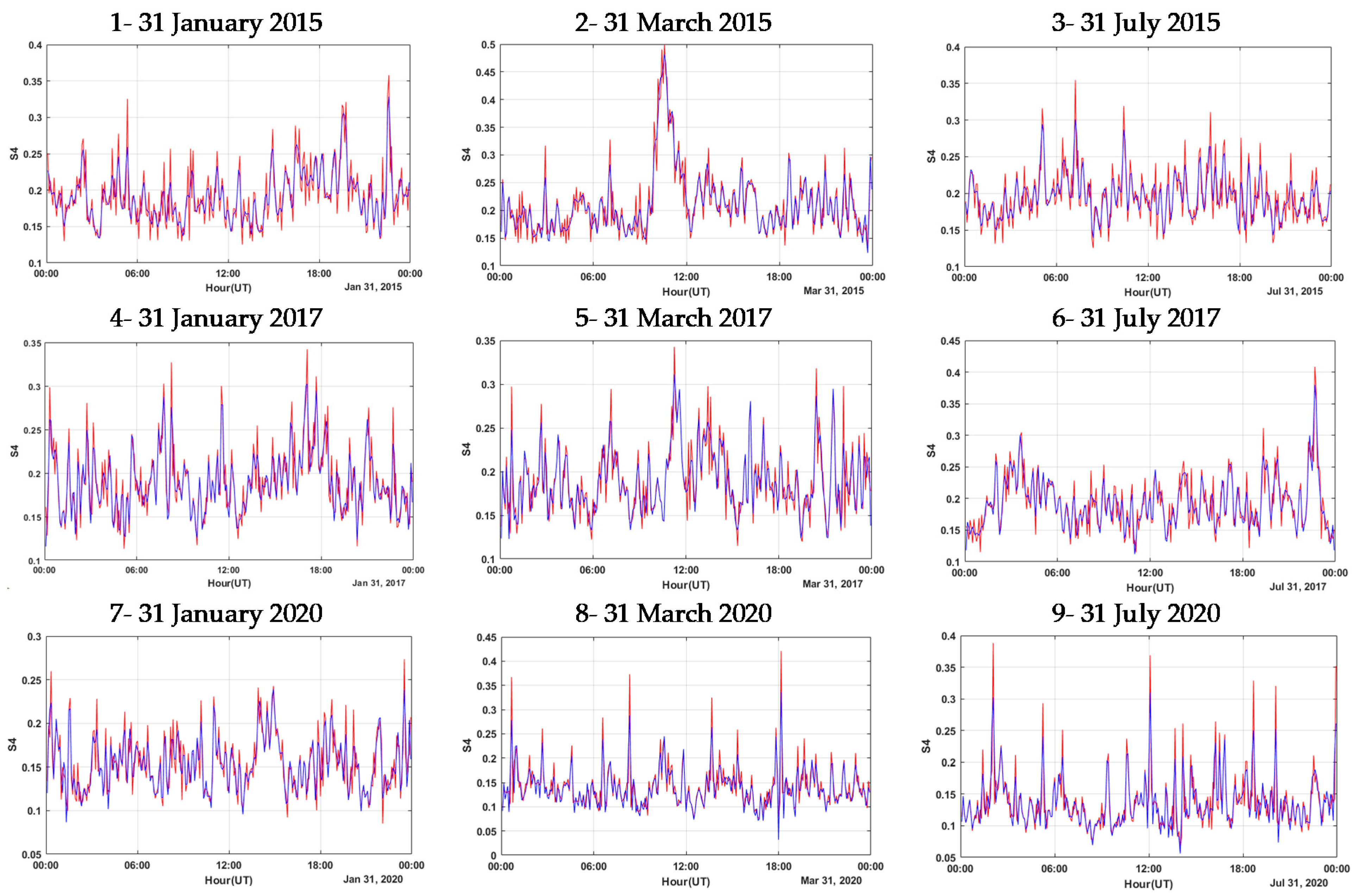
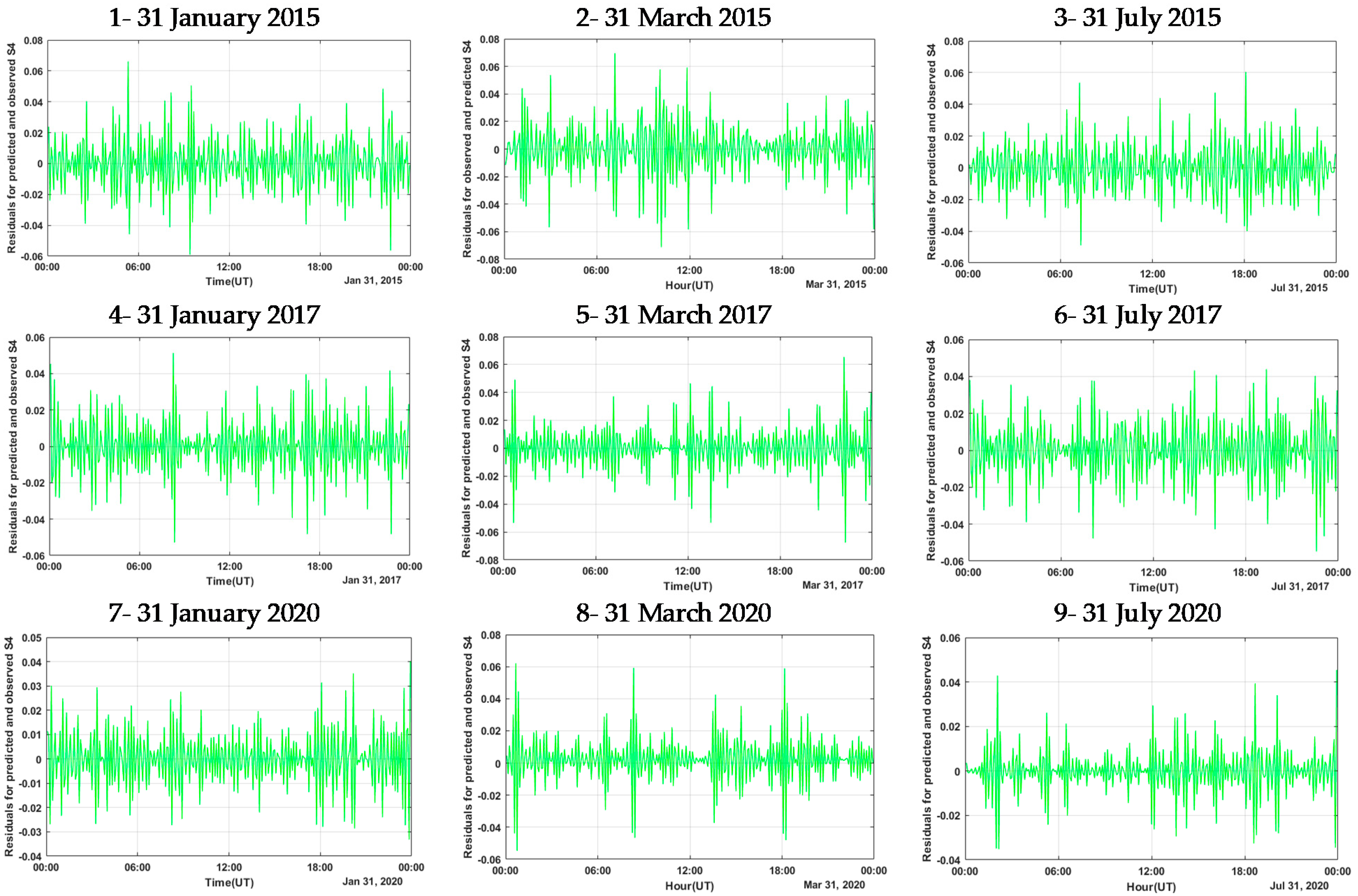
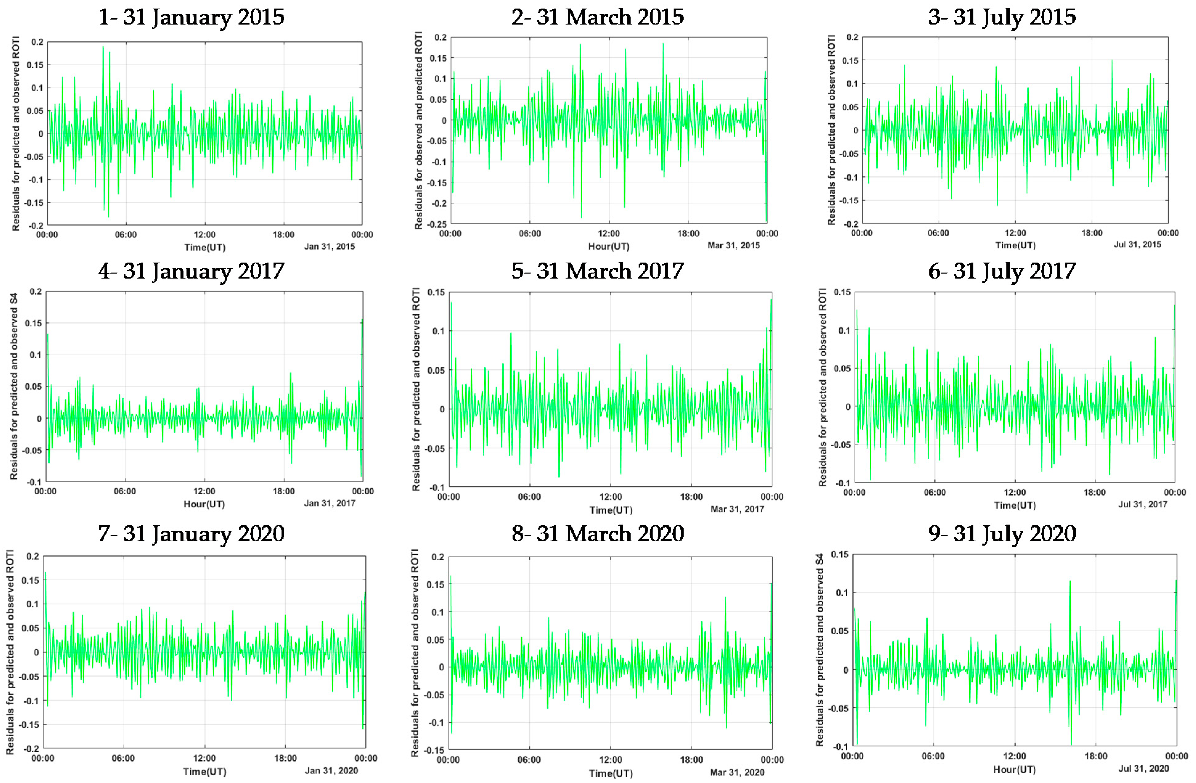
4. Results and Discussion

The data related to the modeling and prediction of ionospheric scintillation in this study include observations with time steps unified for use as input and target data in the ANN. For this purpose, the S4 data were derived from the GNSS observations at GUAM station in Guam, Dededo City, with a longitude of 144.8683 degrees, a latitude of 13.5893 degrees, and a height of 201.922 m higher than the mean sea level. The JAVAD GNSS receiver was used in this station. The RINEX data received from this station with an observation rate of 30 s can be downloaded from the IGS site at ftp://cddis.gsfc.nasa.gov (access on 27 March 2021). Figure 1 shows the location of the two stations with ionosonde and GNSS receivers in Guam near the equatorial ionization anomaly (EIA).

In this research, an ANN is used and integrated with the genetic algorithm (GA) to obtain optimal values of initial weights by introducing preliminary data for modeling and, ultimately, predicting ionospheric scintillation. Additionally, combining the GA with an NN plays a vital role in increasing the accuracy of the modeling and, finally, the daily prediction of ionospheric scintillation. The initial layer has five neurons and includes the network inputs, which combine two subnetworks, while the first hidden layer contains five neurons that are connected to a single neuron in the second hidden layer, sequentially. The sigmoid function is implemented by the first and second hidden layers as a transfer function, while the second hidden layer employs a linear function. The last layer contains a single neuron, which is the output of this model. The implemented ANN uses the weights determined by the GA as the initial weight required by the network [52]. Therefore, for the GANN training process, 80% of the entire dataset was selected randomly to improve the models, and 20% of the whole dataset was applied for the testing process used for the performance evaluation of GANN. Figure 2 presents the architecture of the proposed neural network model for the prediction of ionospheric scintillation parameters (S4 and ROTI).

The implemented ANN uses the weights determined by the GA as the initial weight required by the network [52]. In this designed network, we introduced five types of data as input. These data include the F2 peak electron density height, F2 vertical drift velocity, solar flux parameter (F10.7), sunspot number, and international geomagnetic index $K_P$. On the other hand, the effect of ionospheric phase–amplitude scintillation, which can be expressed in terms of the parameter S4, is entered into the network as target data. The satellite elevation cut-off angle is assumed to be 20 degrees to reduce tracking errors such as multipath. In another approach, we enter these physical parameters as input data and enter the ROTI parameters as target data into the network. In the ANN, a set of data is entered as initial weights, which are introduced to the network with the primary training in the GA, which was discussed in detail in Section 3.2. The average S4 and ROTI data are computed in five-minute time intervals, which is a conventional interval [24], for 24 h for three complete months in three different seasons of the winter solstice, equinox, and summer solstice in 2015 (maximum solar activity), 2017 (moderate solar activity), and 2020 (minimum solar activity). Input data in months January, March, and July in 2017 were used for the initial modeling of the ANN. The prediction was accomplished on the day after each 30-day period, i.e., on 31 January, 31 March, and 31 July. The results of modeling the averaged S4 and ROTI data indicate the application of 30-day modeling for this phenomenon. The input data for the designed GANN contain a two-dimensional matrix where each column represents the five types of geophysical parameters for the 8640 time step. The network then integrates these data into the training process and performs the modeling based on the GA integrated into the ANN (GANN).

In the first step, we compared the results of S4 modeling by GANN for the modeling period of 30 days with the observations of these data at the same time interval. In order to measure the accuracy of the modeling, the parameters of root mean square error (RMSE) and R-square were used for measuring error rates and calculating regression, respectively. In addition, another parameter can be used to evaluate the accuracy of the model trained by the GANN model, by drawing the absolute vector of residuals between the performed modeling and the observational data.

Table 1. The difference between observed and GANN-modeled S4 during the 30 days for January, March, and June in 2015, 2017, and 2020.

	2015			2017			2020
Period of Time	1–30 January	1–30 March	1–30 July	1–30 January	1–30 March	1–30 July	1–30 January	1–30 March	1–30 July
Mean S4	0.22	0.24	0.20	0.19	0.21	0.17	0.15	0.16	0.14
Max S4	0.42	0.51	0.38	0.44	0.49	0.41	0.41	0.43	0.36
RMSE	0.009	0.008	0.009	0.008	0.007	0.008	0.007	0.006	0.007
R-Squared	0.92	0.91	0.92	0.92	0.92	0.93	0.93	0.92	0.94
Scintillation Occurrence (S4 > 0.2)	56%	61%	53%	45%	51%	41%	25%	28%	21%

presents the values of these parameters for the modeled S4 values. Additionally, the percentage of occurrence of ionospheric scintillation was used during the 30-day modeling period, which indicates the number of epochs with S4 > 0.2, thus indicating the occurrence of ionospheric scintillation.

According to the values in Table 1, it can be seen that percentage of ionospheric scintillation that occurred in 2015 (maximum solar activity) is more than that in 2017 (moderate solar activity) and 2020 (minimum solar activity). S4 observation values for the 30-day interval of January, March, and July show that the percentage of ionospheric scintillation occurrence in March is higher than in January and July. According to the obtained values from modeling in Table 1, by considering RMSE and R-square values, it can be seen that the accuracy of modeling the 30-day interval of July is better than that of the other two 30-day intervals of January and March. The lowest modeling accuracy was observed for the 30 days of March 2020, and the highest accuracy was observed for the 30 days of July 2015. Concerning the modeling values implemented in three months in three years with different solar activities, it can be shown that the modeling presented with GANN was less accurate at times when strong ionospheric scintillations occurred. When there are more irregularities, there are more changes in physical parameters that are used as the input of the GANN, and as a result, the modeling accuracy is reduced. However, in times with less ionospheric perturbations, the physical parameter change is less which increases the modeling accuracy. For example, 2020 is more accurate than the other years, and July is more accurate than the other months of that year. Additionally, in 2015 and March, each year has less accuracy in modeling.

In the second step, we predict the S4 for the first day after the modeling period, i.e., for the 31 January, 31 March, and 31 July in 2015, 2017, and 2020, by using the GANN model.

Table 2. The difference between predicted and observed S4 values during 24 h on 31 January, 31 March, and 31 July in 2015, 2017, and 2020.

	2015			2017			2020
Period of Time	31 January	31 March	31 July	31 January	31 March	31 July	31 January	31 March	31 July
Mean S4	0.19	0.21	0.19	0.17	0.18	0.17	0.13	0.15	0.12
Max S4	0.35	0.49	0.35	0.34	0.34	0.41	0.27	0.42	0.39
RMSE	0.022	0.024	0.022	0.019	0.022	0.018	0.015	0.016	0.013
R-Squared	0.81	0.80	0.81	0.81	0.80	0.81	0.83	0.82	0.85
Scintillation Occurrence (S4 > 0.2)	48%	53%	47%	39%	43%	39%	9%	10%	7%

presents the difference between the predicted and observed S4 values. According to [23], S4 values greater than 0.2 are considered as an ionospheric scintillation occurrence. Figure 3 depicts the S4 value for three specified days for detecting ionospheric scintillation. In this plot, the threshold limit of S4 = 0.2 was used to determine the occurrence time of ionospheric scintillation. Table 2 shows that the percentage of ionospheric scintillation in 2015 is clearly more than that in 2017 and 2020. The S4 values for 31 March are higher than those for 31 January, and also 31 July has the lowest S4 value during the 24-h prediction period in these three years.

As it can be seen in Table 2, the highest percentage of ionospheric scintillation was in 2015 and on 31 March. For 31 January and 31 July 2015, it can be seen that ionospheric scintillation occurs during about half of the day. In 2017, the percentage of ionospheric scintillation and the average and maximum S4 decrease compared to 2015. On 31 March 2017, the percentage of ionospheric scintillation reached 43%, which is ten percent less than the same day in 2015. The percentage of ionospheric scintillation and S4 on 31 July and 31 January 2017 also decreased compared to the same day in 2015. By the reduction in solar activity in 2020, the percentage of ionospheric scintillation and S4 values decline during these three years. In 2020, the percentage of ionospheric scintillation during these three days reached a quarter of that on the same day in 2017, meaning that on 31 March, the percentage of ionospheric scintillation occurrence decreased to 10%. The lowest average S4 is 0.12, and the lowest percentage of ionospheric scintillation is 7% on 31 July 2020. RMSE and R-square values in Table 2 show that the 24-h forecast accuracy for 2020 was higher than that in 2017 and 2015. This can be seen by the trend for the 30-day modeling accuracy during these three years. On 31 July 2020, the highest R-square and the lowest RMSE values are obtained among these nine observation days in 2015, 2017, and 2020. On 31 January and then on 31 March of the same year, the highest accuracy is recorded after 31 July 2020. In 2015, the prediction’s accuracy decreases compared to 2020, and this descending trend is repeated for 2015. The prediction accuracy on 31 March 2015 is the lowest prediction accuracy among these three years with a value of 0.80 for R-square and 0.022 for RMSE. Figure 3 demonstrates these values in which the observed and predicted values of S4 are presented for the three 24-h intervals.

In the next step, we consider ROTI values to identify and better predict the ionospheric scintillation phenomenon. The ROTI values are considered in the same period as the previous study of the S4, i.e., the three months of January, March, and June in 2015, 2017, and 2020. The highest mean ROTI observed in March 2015 is equal to 1.14, followed by January (0.97) and July (0.96). The average observational values of the ROTI in 2017 decrease compared to 2015, and this descending trend continues in 2020.

In 2017, the average observational ROTI occurred in March, January, and July, in that order. The lowest average observational ROTI value among these three years observed in July 2020 is equal to 0.74. The ROTI modeling accuracy increases when geomagnetic activity decreases over 30-day intervals. Similar to the first step, parameters such as RMSE, R-square, and residuals were considered by GANN for modeling the ROTI.

Table 3. The difference between observed and GANN-modeled ROTI during the 30 days for January, March, and June in 2015, 2017, and 2020.

	2015			2017			2020
Period of Time	1–30 January	1–30 March	1–30 July	1–30 January	1–30 March	1–30 July	1–30 January	1–30 March	1–30 July
Mean ROTI	0.97	1.14	0.96	0.81	0.91	0.79	0.77	0.78	0.74
Max ROTI	9.47	11.42	7.39	7.91	8.43	7.12	7.63	7.78	6.71
RMSE	0.008	0.009	0.008	0.007	0.008	0.007	0.007	0.007	0.006
R-Squared	0.91	0.90	0.91	0.91	0.90	0.92	0.92	0.92	0.93

presents the data from the modeling conducted in the present study. According to the R-square and RMSE values, it can be seen that the accuracy of modeling for the 30-day interval in 2020 is better compared to the 30 days in 2015 and 2017. Therefore, 2020 is the most accurate in modeling compared to 2015 and 2017. The lowest ROTI modeling accuracy among these three years belongs to the 30 days of March 2015, and the highest modeling accuracy is for the 30 days of July 2020.

In the next step, ROTI values are predicted using the GANN model for the day after the 30-day modeling period. For this purpose, the physical parameters related to the ionospheric irregularities mentioned in the previous sections are used for the prediction day as input data. Then, the ROTI is predicted for the desired time interval using the GANN-trained model.

Table 4. The difference between predicted and observed ROTI and observed VTEC values during 24 h on 31 January, 31 March, and 31 July in 2015, 2017, and 2020.

	2015			2017			2020
Period of Time	31 January	31 March	31 July	31 January	31 March	31 July	31 January	31 March	31 July
Mean ROTI	0.92	1.67	0.91	0.76	0.79	0.75	0.74	0.75	0.73
Max ROTI	1.30	2.18	1.24	1.10	1.03	0.94	1.18	1.05	1.03
RMSE	0.021	0.032	0.021	0.018	0.020	0.018	0.018	0.018	0.017
R-Squared	0.82	0.80	0.82	0.83	0.82	0.83	0.83	0.83	0.84
Mean VTEC	35.33	39.95	18.37	15.74	19.21	12.71	12.48	16.29	9.78
Max VTEC	66.83	77.16	40.25	31.66	47.72	25.41	25.58	33.51	18.42

represents the predicted values for 31 January, 31 March, and 31 July for the ROTI parameter in 2015, 2017, and 2020. As stated in Table 4, the highest observed ROTI is in 2015, followed by 2017 and 2020, respectively. This trend is similar to the average trend of the S4 observed at the same time. According to the average of VTEC observed, it can be seen that mean VTEC values in 2015 were higher than those in the other two years, which indicates the higher solar magnetic activity of that year. Furthermore, 2015, 2017, and 2020 have the highest maximum VTEC and the highest average VTEC. Among the months of each year, March has the highest ROTI and observed VTEC. The highest average ROTI and VTEC observed for these three years are equal to 1.67 and 39.95 TECU, on 31 March 2015. On 31 January and then 31 July, the next highest observed ROTI and VTEC are recorded. The VTEC and ROTI observed in 2020 represent the lowest observed ROTI and VTEC among all predicted days. The lowest means of the ROTI and VTEC observed on 31 July 2020 are equal to 0.73 and 9.78, respectively. Regarding the accuracy of the prediction and the accuracy of modeling, as it can be seen, the accuracy trend for the prediction phase is similar to the modeling stage, i.e., the accuracy of the prediction for the intervals with more accurate modeling is higher. The average observed ROTI value is similar to the modeling trend. Similar to the S4 and ROTI, the R-square and RMSE decrease with a reduction in solar magnetic activity.

Consequently, prediction accuracy parameters are improved. The accuracy of the predicted values for the days of 2020 is higher than that of 2015 and 2020. By referring to the RMSE and R-square, it can be seen that the maximum accuracy is measured on 31 July 2020, with an R-square and RMSE equal to 0.84 and 0.017, respectively. However, the lowest accuracy of prediction is measured on 31 March 2015, where the ROTI and VTEC have their maximum values. The R-square and RMSE are equal to 0.80 and 0.032 on 31 March 2015. According to accuracy parameters for a year, it can be said that 31 July of every year is more accurate than 31 January and 31 March of the same year. These values can be observed in Figure 4. The observed and predicted values of the ROTI are given for the three 24-h intervals. In Figure 4, the mean of VTEC GNSS is observed for GUAM station to obtain additional information on the ROTI and TEC fluctuation intensity.

5. Evaluation of Results

In order to evaluate the GANN modeling and prediction, residual values from the difference between the predicted and observed S4 and ROTI parameters are calculated. The mean and maximum residual values for the S4 and ROTI are given in

Table 5. The residual values of observed minus predicted S4 and ROTI during 24 h on 31 January, 31 March, and 31 July in 2015, 2017, and 2020.

	2015			2017			2020
Period of Time	31 January	31 March	31 July	31 January	31 March	31 July	31 January	31 March	31 July
Mean Absolute Residual S4	0.03	0.04	0.03	0.03	0.03	0.02	0.02	0.02	0.02
Max Absolute Residual S4	0.06	0.07	0.06	0.05	0.06	0.05	0.05	0.06	0.04
Mean Absolute Residual ROTI	0.04	0.05	0.04	0.03	0.03	0.02	0.03	0.03	0.02
Max Absolute Residual ROTI	0.18	0.19	0.16	0.15	0.14	0.13	0.16	0.16	0.11

. As it can be seen from Table 5, the highest average of S4 residuals is obtained for 2015, 2017, and 2020, in that order. It can be seen that the GANN prediction for the S4 in 2020 is higher than that in 2017 and 2015. This is due to less ionospheric perturbations and solar magnetic activity occurring in 2020, compared to 2015 and 2017. The maximum residual value on 31 July is equal to 0.04, which is less than the residuals on all other days, indicating that 31 July has the highest accuracy among the other days of each year. The highest value observed for residuals was measured on 31 March 2015, equal to 0.07, indicating that the prediction accuracy is lower on this day compared to the other days. Figure 5 depicts the residuals between the observed versus predicted values for the S4, along with the values of the vector of residuals.

The maximum and average residual versus the observed and predicted ROTI is presented in Table 5 for 31 January, 31 March, and 31 July in 2015, 2017, and 2020. From Table 5, it can be seen that the ROTI prediction for 2020 compared to 2017 and 2015 has the lowest calculated residual value, which indicates the higher accuracy of the ROTI prediction for this year. The maximum residual value was calculated on 31 March 2015, which is equal to 0.19. Figure 6 represents the vector of residuals for the observed minus predicted ROTI.

6. Conclusions

The current research was conducted to predict ionospheric scintillation for GUAM station, with a longitude of 144.86° and a latitude of 13.58°. For this purpose, the data from the GNSS permanent station and the data from the ionosonde were used to obtain the ionospheric physical data. This region is located in the magnetic equator region, which has a high ionospheric scintillation occurrence rate. In this research, five types of ionospheric physical data were used as the input data in the ANN integrated with the GA for modeling and predicting S4 values. We used the input data in five-minute time intervals to predict the occurrence of ionospheric scintillation using S4 and ROTI parameters at the consequent day after the 30-day modeling period. The use of data related to S4 and ROTI parameters is related to the type of intrinsic noise structure; thus, severe changes in their values in the short time intervals are inevitable, and modeling this type of data seems relatively complicated. However, using the ANN method and integrating it with the GA made it possible to create flexibility in modeling this dataset. The data were selected in three different months from different seasons of winter, spring equinox, and summer during three different years, 2015 (maximum solar activity), 2017 (moderate solar activity), and 2020 (minimum solar activity). The modeling performed for the S4 parameter in the 30-day intervals had a regression value greater than 91% and an RMS error of about 0.01. In addition, the regression of this parameter was more than 80% for the one-day prediction. For the ROTI parameter, the regression value of modeling was above 90%, and the RMS error was 0.03, although the regression of the daily prediction was more than 80%. According to the R-square and RMSE parameters for modeling and predicting the S4 and ROTI, when solar magnetic activity decreases, ionospheric irregularities reduce, and consequently, the accuracy of the predicted parameter is improved. This can be clearly seen from the results, where the accuracy of predicted values for 31 January, 31 March, and 31 July 2020 are higher than the same days in 2015 and 2017. The presented results are limited to the applied database but show that an operational evaluation of the recommended method would be worthwhile. Concluding, the ANN method integrated with the GA can detect and predict ionospheric scintillation occurrence near real time on a daily basis, which is critical for reducing the error of the ionospheric scintillation impact on satellite-based communication and navigation system performance. This method can play a precautionary role for alerting GNSS users that the observation epoch might be disturbed by ionospheric scintillation, and GNSS users can eliminate error-infected observations from the dataset.

References

1. De Paula, E.; Rodrigues, F.; Iyer, K.; Kantor, I.; Abdu, M.; Kintner, P.; Ledvina, B.; Kil, H. Equatorial anomaly effects on GPS scintillations in brazil. Adv. Space Res. 2003, 31, 749–754. [Google Scholar] [CrossRef]
2. Xu, R.; Liu, Z.; Li, M.; Morton, Y.; Chen, W. An Analysis of Low-Latitude Ionospheric Scintillation and Its Effects on Pre-cise Point Positioning. J. Glob. Position. Syst. 2012, 11, 22–32. [Google Scholar] [CrossRef]
3. Appleton, E.V. The anomalous equatorial belt in the F2-layer. J. Atmospheric Terr. Phys. 1954, 5, 348–351. [Google Scholar] [CrossRef]
4. Ma, G.; Maruyama, T. A super bubble detected by dense GPS network at east Asian longitudes. Geophys. Res. Lett. 2006, 33. [Google Scholar] [CrossRef]
5. Demyanov, V.V.; Yasyukevich, Y.V.; Ishin, A.B.; Astafyeva, E.I. Ionospheric super-bubble effects on the GPS positioning relative to the orientation of signal path and geomagnetic field direction. GPS Solut. 2011, 16, 181–189. [Google Scholar] [CrossRef]
6. Abdu, M. Outstanding problems in the equatorial ionosphere-thermosphere electrodynamics relevant to spread F. J. Atmos. Sol. Terr. Phys. 2001, 63, 869–884. [Google Scholar] [CrossRef]
7. Anderson, P.C.; Straus, P.R. Magnetic field orientation control of GPS occultation observations of equatorial scintillation. Geophys. Res. Lett. 2005, 32. [Google Scholar] [CrossRef]
8. De Lima, G.R.T.; Stephany, S.; De Paula, E.R.; Batista, I.S.; Abdu, M.A. Prediction of the level of ionospheric scintillation at equatorial latitudes in Brazil using a neural network. Space Weather 2015, 13, 446–457. [Google Scholar] [CrossRef]
9. Ratnam, D.V.; Sivavaraprasad, G.; Lee, J. Automatic ionospheric scintillation detector for global navigation satellite system receivers. IET Radar Sonar Navig. 2015, 9, 702–711. [Google Scholar] [CrossRef]
10. Sivavaraprasad, G.; Padmaja, R.S.; Ratnam, D.V. Mitigation of Ionospheric Scintillation Effects on GNSS Signals Using Variational Mode Decomposition. IEEE Geosci. Remote Sens. Lett. 2017, 14, 389–393. [Google Scholar] [CrossRef]
11. Sivavaraprasad, G.; Ratnam, D.V.; Otsuka, Y. Multicomponent Analysis of Ionospheric Scintillation Effects Using the Synchrosqueezing Technique for Monitoring and Mitigating their Impact on GNSS Signals. J. Navig. 2019, 72, 669–684. [Google Scholar] [CrossRef]
12. Knight, M.F. Ionospheric Scintillation Effects on Global Positioning System Receivers; Department of Electrical and Electronic Engineering, University of Adelaide: Adelaide, Australia, 2000. [Google Scholar]
13. Sridhar, M.; Ratnam, D.V.; Raju, K.P.; Praharsha, D.S.; Saathvika, K. Ionospheric scintillation forecasting model based on NN-PSO technique. Astrophys. Space Sci. 2017, 362, 166. [Google Scholar] [CrossRef]
14. Costa, E.; Basu, S. A radio wave scattering algorithm and irregularity model for scintillation predictions. Radio Sci. 2002, 37, 1–13. [Google Scholar] [CrossRef]
15. Béniguel, Y.; Adam, J.-P.; Jakowski, N.; Noack, T.; Wilken, V.; Valette, J.-J.; Cueto, M.; Bourdillon, A.; Lassudrie-Duchesne, P.; Arbesser-Rastburg, B. Analysis of scintillation recorded during the PRIS measurement campaign. Radio Sci. 2009, 44, 1–11. [Google Scholar] [CrossRef]
16. Forte, B.; Radicella, S.M. Comparison of ionospheric scintillation models with experimental data for satellite navigation applications. Ann. Geophys. 2005. [Google Scholar] [CrossRef]
17. Secan, J.A.; Bussey, R.M.; Fremouw, E.J.; Basu, S. An improved model of equatorial scintillation. Radio Sci. 1995, 30, 607–617. [Google Scholar] [CrossRef]
18. Secan, J.A.; Bussey, R.M.; Fremouw, E.J.; Basu, S. High-latitude upgrade to the Wideband ionospheric scintillation model. Radio Sci. 1997, 32, 1567–1574. [Google Scholar] [CrossRef]
19. Das, A.; Das Gupta, A.; Ray, S. Characteristics of L-band (1.5 GHz) and VHF (244 MHz) amplitude scintillations recorded at Kolkata during 1996–2006 and development of models for the occurrence probability of scintillations using neural network. J. Atmos. Sol. Terr. Phys. 2010, 72, 685–704. [Google Scholar] [CrossRef]
20. Rezende, L.F.C.; de Paula, E.R.; Stephany, S.; Kantor, I.J.; Muella, M.T.A.H.; de Siqueira, P.M.; Correa, K.S. Survey and prediction of the ion-ospheric scintillation using data mining techniques. Space Weather 2010, 8, 1–10. [Google Scholar] [CrossRef]
21. Redmon, R.J.; Anderson, D.; Caton, R.; Bullett, T. A Forecasting Ionospheric Real-time Scintillation Tool (FIRST). Space Weather 2010, 8. [Google Scholar] [CrossRef]
22. De Lima, G.R.T.; Stephany, S.; de Paula, E.R.; Batista, I.S.; Abdu, M.A.; Rezende, L.F.C.; Aquino, M.G.S.; Dutra, A.P.S. Correlation analysis between the occurrence of ionospheric scintillation at the magnetic equator and at the southern peak of the equatorial ion-ization anomaly. Space Weather 2014, 12, 406–416. [Google Scholar] [CrossRef]
23. Priyadarshi, S. A Review of Ionospheric Scintillation Models. Surv. Geophys. 2015, 36, 295–324. [Google Scholar] [CrossRef] [Green Version]
24. Van Dierendonck, A.; Klobuchar, J.; Hua, Q. Ionospheric scintillation monitoring using commercial single frequency C/A code receivers. In Proceedings of the 6th International Technical Meeting of the Satellite Division of The Institute of Navigation (ION GPS 1993), Salt Lake City, UT, USA, 22–24 September 1993; pp. 1333–1342. [Google Scholar]
25. Tiwari, R.; Strangeways, H.J. Regionally based alarm index to mitigate ionospheric scintillation effects for GNSS receivers. Space Weather 2015, 13, 72–85. [Google Scholar] [CrossRef] [Green Version]
26. Juan, J.M.; Aragon-Angel, A.; Sanz, J.; González-Casado, G.; Rovira-Garcia, A. A method for scintillation characterization using geodetic receivers operating at 1 Hz. J. Geod. 2017, 91, 1383–1397. [Google Scholar] [CrossRef] [Green Version]
27. Van Dierendonck, A.J.; Arbesser-Rastburg, B. Measuring ionospheric scintillation in the equatorial region over Africa, in-cluding measurements from SBAS geostationary satellite signals. In Proceedings of the ION GNSS 17th Technical Meeting of the Satellite Division, Long Beach, CA, USA, 21–24 September 2004; pp. 316–324. [Google Scholar]
28. Demyanov, V.V.; Sergeeva, M.A.; Yasyukevich, A.S. GNSS High-Rate Data and the Efficiency of Ionospheric Scintillation Indices. In Book Satellites Missions and Technologies for Geosciences; Intech Open Limited: London, UK, 2020. [Google Scholar]
29. Taabu, S.D.; D’ujanga, F.M.; Ssenyonga, T. Prediction of ionospheric scintillation using neural network over East African region during ascending phase of sunspot cycle 24. Adv. Space Res. 2016, 57, 1570–1584. [Google Scholar] [CrossRef]
30. Alfonsi, L.; Spogli, L.; Tong, J.R.; De Franceschi, G.; Romano, V.; Bourdillon, A.; Le Huy, M.; Mitchell, C.N. GPS scintillation and TEC gradients at equatorial latitudes in April 2006. Adv. Space Res. 2011, 47, 1750–1757. [Google Scholar] [CrossRef]
31. Yang, Z.; Liu, Z. Correlation between ROTI and Ionospheric Scintillation Indices using Hong Kong low-latitude GPS data. GPS Solut. 2016, 20, 815–824. [Google Scholar] [CrossRef]
32. Zou, Y.; Wang, D. A study of GPS ionospheric scintillations observed at Guilin. J. Atmos. Sol. Terr. Phys. 2009, 71, 1948–1958. [Google Scholar] [CrossRef]
33. Basu, S.; Groves, K.; Quinn, J.; Doherty, P. A comparison of TEC fluctuations and scintillations at Ascension Island. J. Atmos. Sol. Terr. Phys. 1999, 61, 1219–1226. [Google Scholar] [CrossRef]
34. Pi, X.; Mannucci, A.J.; Lindqwister, U.J.; Ho, C.M. Monitoring of global ionospheric irregularities using the Worldwide GPS Network. Geophys. Res. Lett. 1997, 24, 2283–2286. [Google Scholar] [CrossRef]
35. Li, G.; Ning, B.; Yuan, H. Analysis of ionospheric scintillation spectra and TEC in the Chinese low latitude region. Earth Planets Space 2007, 59, 279–285. [Google Scholar] [CrossRef] [Green Version]
36. Sultan, P.J. Linear theory and modeling of the Rayleigh-Taylor instability leading to the occurrence of equatorial spread F. J. Geophys. Res. Space Phys. 1996, 101, 26875–26891. [Google Scholar] [CrossRef]
37. Zolesi, B.; Cander, L.R. The General Structure of the Ionosphere. In Ionospheric Prediction and Forecasting; Springer: Berlin/Heidelberg, Germany, 2013; pp. 11–48. [Google Scholar]
38. Wilkinson, J. New Eyes on the Sun: A Guide to Satellite Images and Amateur Observation; Springer Science & Business Media: Berlin, Germany, 2012. [Google Scholar] [CrossRef]
39. Aquino, M.H.; Waugh, S.; Dodson, A.; Moore, T.; Skone, S. GPS based ionospheric scintillation monitoring. In Proceedings of the Space Weather Workshop: Looking towards a European Space Weather Programme, Noordwijk, The Netherlands, 17–19 December 2004. [Google Scholar]
40. Li, G.; Ning, B.; Zhao, B.; Liu, L.; Liu, J.Y.; Yumoto, K. Effects of geomagnetic storm on GPS ionospheric scintillations at Sanya. J. Atmos. Sol. Terr. Phys. 2008, 70, 1034–1045. [Google Scholar] [CrossRef]
41. Li, G.; Ning, B.; Wang, C.; Abdu, M.A.; Otsuka, Y.; Yamamoto, M.; Wu, J.; Chen, J. Storm-enhanced development of postsunset equatorial plasma bubbles around the meridian 120°E/60°W on 7–8 September 2017. J. Geophys. Res. Space Phys. 2018, 123, 7985–7998. [Google Scholar] [CrossRef]
42. Tilahun, S.; Tariku, Y.A. Verification of ionospheric perturbation induced L-band frequency scintillation using HF/VHF bands over the African equatorial and low latitude region, Ethiopia. J. Atmos. Sol. Terr. Phys. 2019, 195, 105135. [Google Scholar] [CrossRef]
43. Haykin, S.S. Neural Networks and Learning Machines/Simon Haykin; Prentice Hall: New York, NY, USA, 2009. [Google Scholar]
44. Beale, R.; Jackson, T. Neural Computing—An Introduction; CRC Press: London, UK, 1990. [Google Scholar]
45. Norgaard, M. Neural Network Based System Identification Toolbox; Department of Automation, Technical University of Denmark: Lyngby, Denmark, 2000. [Google Scholar]
46. Gen, M.; Lin, L. Genetic Algorithms. Wiley Encycl. Comput. Sci. Eng. 2007, 1–15. [Google Scholar] [CrossRef]
47. Schaffer, J.; Whitley, D.; Eshelman, L. Combinations of genetic algorithms and neural networks: A survey of the state of the art. In Proceedings of the COGANN-92: International Workshop on Combinations of Genetic Algorithms and Neural Networks, Baltimore, MD, USA, 6 June 1992; IEEE: Piscataway, NJ, USA, 2003; pp. 1–37. [Google Scholar]
48. Alonso, J.M.; Alvarruiz, F.; Desantes, J.M.; Hernández, L.; Hernández, V.; Molto, G. Combining neural networks and genetic algorithms to predict and reduce diesel engine emissions. IEEE Trans. Evol. Comput. 2007, 11, 46–55. [Google Scholar] [CrossRef]
49. Montana, D.J.; Davis, L. Training Feedforward Neural Networks Using Genetic Algorithms. IJCAI 1989, 89, 762–767. [Google Scholar]
50. Le, L.T.; Nguyen, H.; Dou, J.; Zhou, J. A Comparative Study of PSO-ANN, GA-ANN, ICA-ANN, and ABC-ANN in Estimating the Heating Load of Buildings’ Energy Efficiency for Smart City Planning. Appl. Sci. 2019, 9, 2630. [Google Scholar] [CrossRef] [Green Version]
51. Mallika, I.L.; Ratnam, D.V.; Ostuka, Y.; Sivavaraprasad, G.; Raman, S. Implementation of hybrid iono-spheric TEC forecasting algorithm using PCA-NN method. IEEE J. Sel. Top. Appl. Earth Obs. Remote Sens. 2018, 12, 371–381. [Google Scholar] [CrossRef]
52. Cook, D.F.; Ragsdale, C.T.; Major, R.L. Combining a neural network with a genetic algorithm for process parameter optimization. Eng. Appl. Artif. Intell. 2000, 13, 391–396. [Google Scholar] [CrossRef]
Figure 1. Location of the two stations with ionosonde and GNSS receivers: Guam near the equatorial ionization anomaly (EIA).
Remotesensing 13 02092 g001
Figure 2. The architecture of the proposed neural network model for the prediction of ionospheric scintillation parameters (S4 and ROTI).
Remotesensing 13 02092 g002
Figure 3. The predicted and observed S4 during 24 h on 31 January, 31 March, and 31 July in 2015, 2017, and 2020.
Remotesensing 13 02092 g003
Figure 4. The predicted and observed ROTI during 24 h on 31 January, 31 March, and 31 July in 2015, 2017, and 2020.
Remotesensing 13 02092 g004
Figure 5. The residual vectors of observed minus predicted S4 values during 24 h on 31 January, 31 March, and 31 July in 2015, 2017, and 2020.
Remotesensing 13 02092 g005
Figure 6. The residual vectors of observed minus predicted ROTI values during 24 h on 31 January, 31 March, and 31 July in 2015, 2017, and 2020.
Remotesensing 13 02092 g006