Effect of the Assimilation Frequency of Radar Reflectivity on Rain Storm Prediction by Using WRF-3DVAR

Abstract

An attempt was made to evaluate the impact of assimilating Doppler Weather Radar (DWR) reflectivity together with Global Telecommunication System (GTS) data in the three-dimensional variational data assimilation (3DVAR) system of the Weather Research Forecast (WRF) model on rain storm prediction in Daqinghe basin of northern China. The aim of this study was to explore the potential effects of data assimilation frequency and to evaluate the outputs from different domain resolutions in improving the meso-scale NWP rainfall products. In this study, four numerical experiments (no assimilation, 1 and 6 h assimilation time interval with DWR and GTS at 1 km horizontal resolution, 6 h assimilation time interval with radar reflectivity, and GTS data at 3 km horizontal resolution) are carried out to evaluate the impact of data assimilation on prediction of convective rain storms. The results show that the assimilation of radar reflectivity and GTS data collectively enhanced the performance of the WRF-3DVAR system over the Beijing-Tianjin-Hebei region of northern China. It is indicated by the experimental results that the rapid update assimilation has a positive impact on the prediction of the location, tendency, and development of rain storms associated with the study area. In order to explore the influence of data assimilation in the outer domain on the output of the inner domain, the rainfall outputs of 3 and 1 km resolution are compared. The results show that the data assimilation in the outer domain has a positive effect on the output of the inner domain. Since the 3DVAR system is able to analyze certain small-scale and convective-scale features through the incorporation of radar observations, hourly assimilation time interval does not always significantly improve precipitation forecasts because of the inaccurate radar reflectivity observations. Therefore, before data assimilation, the validity of assimilation data should be judged as far as possible in advance, which can not only improve the prediction accuracy, but also improve the assimilation efficiency.

1. Introduction

There have been higher requirements put forward for the prediction of convective systems precipitation and its related disasters in recent years. Improving the accuracy of precipitation forecast has long been a challenge for Numerical Weather Prediction (NWP) model researchers and operational communities [1,2]. Kryza and Werner et al. [3] forecasted several short and intensive rainfalls over the SW area of Poland using the Weather Research and Forecasting Model (WRF) with different parameterization and spatial resolution. The results show that none of the experimented model configurations was able to reproduce a local intensive rainfall properly. Hamill and Thomas [4] applied ensemble prediction systems to describe the performance of the WRF precipitation forecasts. Although ensemble forecast can reflect the predictability or reliability of real atmosphere to some extent, it cannot improve the physical mechanism of the model. Among many considerable causes that could lead to the inherent low predictability of convective precipitation forecasting using an NWP system, ambiguous description of the atmosphere initial state is one of them. Rainfall features are always generated in an inaccurate manner, regarding location, initiation, timing, and intensity, especially of convective storms [5]. As a result, accurately obtaining the initial state of a storm for the regional model is the key issue for a successful prediction of the convective system.

Several studies have confirmed it is possible to remedy defects through data assimilation into the NWP model. Among the numerous data assimilation methods, those commonly used by researchers include the optimal interpolation methods, the three-dimensional variational (3DVAR) [6,7], the four-dimensional variational (4DVAR) [8,9], and the Kalman filter [10] approaches. Thereinto, 3DVAR is practicable in terms of computational efficiency, thus is adopted the most frequently [5]. Variational data analysis system was first developed by Sun and Juanzhen et al. [11], which is called Variational Doppler Radar Analysis System (VDRAS) and began this pioneering work. Subsequently, it was expanded by Sun and Crook [12] to use for short-term forecast initialization during convective precipitation. Yang and Duan et al. [13] discussed if 3DVar data assimilation could potentially improve the rainfall forecast in the WRF model, an obvious improvement of the event with even rainfall in temporal distribution was found regarding the northeastern Tibetan Plateau area. Physical initialization combined with the three-dimensional variational data assimilation method (PI3DVAR_rh) was designed by Gan and Yang et al. [14], through which the spatial pattern forecasting of radar reflectivity and precipitation were improved based on WRF. Vedrasco and Sun et al. [15] certified that the 3DVAR analysis with the constraint introduced into WRF could improve the initial state of the model and guide the convective characteristics exhibited by six summer convection cases across Brazil. These studies show that 3DAVR plays a positive role in rainfall forecast, and this system, which is widely used in data assimilation, is also adopted in this study.

With high-resolution observation data becoming increasingly rich, it has been a hot research topic worldwide in recent years to improve the short-term quantitative precipitation prediction level by using high-resolution observation. High-resolution observations like Doppler radar and GTS data, can provide huge amounts of detailed information with high spatial and temporal resolution, which makes it possible to further improve the convective rainstorm forecast. Doppler radar can make millions of measurements of precipitation with a spatial resolution of a few kilometers and a temporal resolution of a few minutes [5]. Compared with existing meso-scale measure platforms, such a significant advantage of spatial and temporal resolution has great potential for improving small-scale and short-term rainfall prediction.

Many researchers combine high-resolution observational data with numerical models, which plays a positive role in promoting the development of convective rainfall prediction, improving the initial state of numerical models, as well as alleviating the imbalance caused by interpolation [16,17,18,19]. Routray and Mohanty [20] believed that the assimilation of radar data (radial velocity and reflectivity factor) has a positive impact on enhancing performance of the WRF-3DVAR (WRF-three-dimensional variational) system for the Indian region. Gvindankutty and Chandrasekar et al. [21] investigated how the 3DVAR assimilation of DWR radial wind and GTS data positively affected the precipitation intensity as well as spatial distribution. Abhilash and Sahai et al. [22] demonstrated improvement in spatial pattern of rainfall of convective systems precipitation by assimilating relevant parameter obtained by the WRF-3DVAR system, including DWR radial velocity and reflectivity as well as GTS data. Osuri and Mohanty et al. [23] used the WRF-3DVAR system to assimilate DWR with GTS, thus conducting 24 cases to predict tropical cyclones of Bay of Bengal, and the results show that this method helps to provide a positive impact on the credibility of prediction. Sugimoto and Crook et al. [5] indicated that in the 3DVAR framework and the storm case, assimilating the radial velocity as well as reflectivity can achieve the best performance, applied on short-range precipitation forecasting. A cycling data assimilation improves the regional models’ initial state on the one hand, and meanwhile introduces observation data to mitigate the imbalance caused by interpolation of prediction on the other hand [24]. The data assimilation system allows higher-resolution observations to be used as the background through update-cycling procedure [25,26], which makes the data assimilation system rely on a specified combination of error statistics to obtain the optimal short-term forecast analysis.

Although data assimilation is capable of improving the NWP (i.e., WRF) convective precipitation in an effectively manner, the quality of data assimilation creates uncertainty about results. Some studies have shown that the quality of assimilated data is critical to forecast results. Liu and Tian et al. [27] indicated that data assimilation via WRF-3DVar could potentially improve the rainfall forecasting in northern China, with GTS data, radar reflectivity, and radial velocity assimilated every 6 h. From their study, it is concluded that it is the effective information in the assimilated data that exhibited more significant results rather than the volume of data. Tian and Liu et al. [28] further explored the effect of assimilating radar data from different height layers on the improvement of the NWP rainfall accuracy. The results showed that the accuracy of the forecasted rainfall deteriorated with the rise of the height of the assimilated radar reflectivity. In the process of data assimilation, the frequency of assimilation determines the amount of effective data assimilated. Considering the time cost, most operation departments choose a 6 h assimilation interval [3,27,29]. In later developments, many researchers and principal operational centers upgraded the regional NWP systems with a 3 h assimilation time interval [30]. For highly convective storms, more frequent data assimilation with a shorter time interval is found to be more effective to produce reliable predictions [31]. Li and Wang et al. [32] demonstrated that the assimilation of radial velocity every half an hour could enhance the intensity analyses and forecasts of rainfall compared to results without assimilating radar data. Kawabata and Seko et al. [33] applied four-dimensional variational (4DVAR) with a horizontal resolution of 2 km and 1 h length of the assimilation window to forecast heavy rainfall at the central part of Tokyo. In most cases, researchers tend to assimilate observations as they are originally obtained, rather than choose an appropriate assimilation frequency or time interval.

Despite the wide application of data assimilation in enhancing precipitation forecasts, the sensitivity of data assimilation frequency has not yet gained enough attention. This study mainly aims at evaluating how the WRF-3DVAR with different assimilation frequencies affects the accuracy of the forecast precipitation. Four typical rain storms that occurred in semi-humid and semi-arid area of northern China were chosen as study objects. Doppler radar and GTS data were assimilated in four designed experiments with the time intervals of 6 and 1 h by WRF-3DVAR. The results would be helpful to improving data assimilation efficiency with WRF-3DVAR, and provide guidance for the development of a similar basin rainstorm forecast system. At the same time, in order to study the sensitivity of data assimilation to rainfall forecast, the quality of radar data is also analyzed.

2. Methodology

To explore the data assimilation frequency of the short-range precipitation forecasting, the numerical model WRF is chosen for this study [7] and its assimilating extension WRF-3DAVR is used. WRF version 3.7 is used for all experiments. The WRF model is a fully compressible, non-hydrostatic, mesoscale NWP, and atmospheric simulation system. In addition, WRF-3DAVR can further influence the initial state of the WRF model by assimilating different high-resolution observations. A brief overview of the basic model settings and the system description can be found in the following sections.

2.1. A Brief Description of WRF-3DVAR

The fundamental objective of the 3DVAR system is to seek an optimal estimate of initialization at parsing time through an iterative solution of a pre-determined function, including observations, background forecast from the NWP system, etc. [34].

$${J\left(x\right)=J}^b{+J}^o=\frac{1}{2}{\left({x-x}^b\right)}^T{B}^{-1}\left({x-x}^b\right)+\frac{1}{2}{\left({y-y}^o\right)}^T{(E+F)}^{-1}\left({y-y}^o\right)$$

(1)

Iterative solutions to Equation (1) can summarize the Dimensional Variational Assimilation problem, to seek the analysis state variable x to minimize J(x). In the formula, x is the variable that represents the surface and atmospheric surface state, x^b is the first guess (or background) acquired from the previous forecast, and y⁰ is the assimilated observation. Y = H(x) is the model-derived observation space, which is transformed from gridded analysis x by the observation operator H for comparison against y⁰. The individual data points are fitted by the weight of its error estimate: B, E, and F are the background error covariance matrix, observation error covariance matrix, and representativity error covariance matrices, respectively. This solution represents a minimum variance estimate of the true state of the atmosphere given the two sources of a priori data: the first guess x^b and the observation y⁰ [35].

The WRF-3DVar is a variational data assimilation system designed and built in the WRF model, and is used to assimilate radar reflectivity and GTS in this study [6,36]. The background error covariance CV3 created by the National Meteorological Center (NMC) was employed, which has the advantage of wide applicability [37].

2.2. WRF Model Configuration

The primary focus of this study is Fuping and Zijingguan catchments covered by the innermost domain of a three nested domain. For the study area, the center of the domain is at 39°26′00″N and 114°46′00″E, and from the outermost to the innermost the nested domain sizes are 1260 × 1260, 450 × 360, and 145 × 115 km². Considering the diversity in assimilation variables, the horizontal grid spacing of the outermost domain is set at 9 km and the grid size of the innermost layer is set to be 1 km, where the downscaling radio is set to be 1:3 [38,39]. The locations of the nested domain and radar coverage are shown in Figure 1. Forty vertical pressure levels are considered for the three nested domains with a model top at 50 hPa [40,41].

The 1°×1° spatial resolution of Global Forecast System (GFS) forecast data provide the initial and lateral boundary conditions for the simulations. Considering the resolution of the GFS data, it would be more reasonable to add another domain with 27 km horizontal grid spacing as the outermost one. Unfortunately, experimental runs are carried out and the effects of data assimilation are found to be similar with the current domain settings. Since rainstorm forecasting has a high requirement of effectiveness for a given period of time, in practical application it is beneficial to obtain the forecasting information as soon as possible. Therefore, the 27 km grid is not applied in this study. The integration time-step of the WRF model and WRF-3DAVR system is 6 s and the time interval for the output is set to be 1 h. The GFS data, which is updated every six hours, is a real-time product provided by National Centers for Environmental Prediction (NCEP). Because GFS has not been processed by assimilation analysis, it has been used in many studies to forecast the storm events in WRF model and WRF-3DAVR [3,5,31].

The performance of the model is highly dependent on the parameterized scheme, and the scheme selected in the study may be suitable for one storm event in one region, but not necessarily for others [42]. Since it is difficult to judge which scheme is most suitable for future storm events, parameterized schemes are usually determined in advance for practical application [43]. Based on relevant experimental research on the selection of sensitive parameterization schemes for ensemble rainfall forecasting [44,45], the physical parameters with the best applicability in the study area were adopted in this study. Details of the parameterizations that have significant impacts on the generation of rainfall used in the assimilation experiments are shown in

Table 1. Details of the parameterizations used in the assimilation experiments.

Parameterization	Chosen Option	Reference
Microphysics scheme	WSM6	[46]
Longwave radiation	Rapid Radiative Transfer Model (RRTM)	[47]
Shortwave radiation	Dudhia	[48]
Land surface scheme	Noah	[49]
Planetary boundary layer	Mellor-Yama-da-Janjic (MYJ)	[50]
Cumulus convection	Kain-Fritsch (KF)	[51]

. It is worth noting that the cumulus scheme is switched off for the 3 and 1 km domain.

3. Case Study and Data

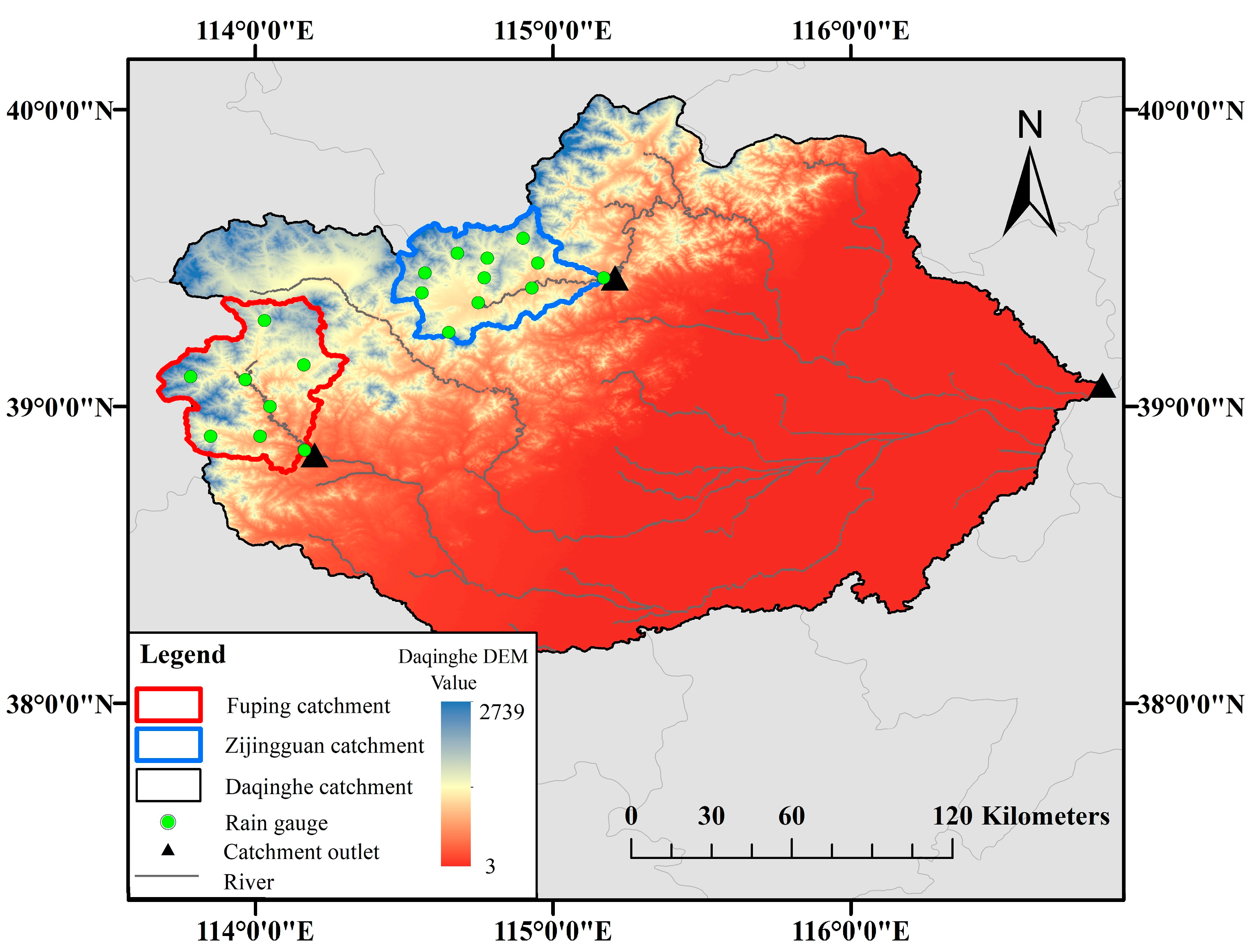
3.1. Study Area and Storm Events

The main focus of this study is the Fuping and Zijingguan watershed covered by Domain 2 and Domain 3 of the WRF model. According to the temporal and spatial distribution characteristics of rainfall and the representatives of rainfall-runoff generation characteristics, the case used in this study is four 24-h rainstorm events, which occurred in Fuping and Zijingguan watershed. Fuping catchment is located at 39°22′N~38°47′N and 113°40′E~114°18′E with a drainage area of 2210 km² and Zijingguan catchment is located at 39°13′~39°40′N and 114°28′~115°11′E with a drainage area of 1760 km². They belong to the south and the north branch of the Daqinghe basin respectively, located in northern China, having a warm temperate continental monsoon climate. Terrain elevation of the study area varies from 2286 m in the northwest part to 200 m in the southeast mountains. The average annual rainfall in the study catchments is approximately 600 mm, the short episodes of intensive precipitation are more frequent in late May and early September. The steep terrain leads to a short confluence time of the flood, which together with high-intensity, short-duration precipitation is prone to cause severe flood disasters. They are concentrated in areas with thin soil layer and low vegetation coverage especially. In particular, on 21 July 2012, the 24 h rainstorm event occurred in the Beijing-Tianjin-Hebei region, which has been widely concerned because of the heavy rainfall intensity and large losses. The duration of the four storm events and the accumulative rainfall amounts are shown in

Table 2. Duration, accumulated rainfall, and maximum stream flow of the four selected 24 h storm events.

Event ID	Catchment	Storm Start Time	Storm End Time	Accumulated Rainfall (mm)
I	Fuping	29/07/2007 20:00	30/07/2007 20:00	63.38
II	Fuping	30/07/2012 10:00	31/07/2012 10:00	50.48
III	Fuping	11/08/2013 07:00	12/08/2013 07:00	30.82
IV	Zijingguan	21/07/2012 04:00	22/07/2012 04:00	155.43

. Among the four storms, event 4 is the heaviest one trigged by a severe convective system, concentrated in a small area of the watershed and with high rainfall intensity in a short time period. The other three storms are typical stratiform rains with moderate intensity but various distributions in space and time. The measured rainfall data are rainfall stations and the time interval is 1 h. The 24 h rainfall accumulation is computed by Thiessen polygon method, which averages the observations from the rain gauges. Figure 2 demonstrates a detailed map of the study area, such as the rain gauges, watershed boundary, catchment outlets topography, and major rivers.

In reality, the precipitation in northern China is not absolutely even in time and space, which is different from that in southern China. To study the spatial and temporal evenness of the precipitation in study catchments, both spatial and temporal variation coefficient (Cv) of four storm events from 1985 to 2015 are calculated. A threshold of 5% was employed to separate even and uneven rainfall events. The evenness of the rainstorm events is quantitatively evaluated in the spatial and temporal dimensions by variation coefficient Cv in this study. The lower Cv is, the more even the rainfall is. Based on the thresholds selected, we found two critical values: 0.4 for spatial Cv and 0.6 for temporal Cv. When the rainfall Cv values were less than the threshold Cv values, storm events have a relatively even distribution of rainfall over the respective catchment.

Table 3. Rainfall evenness of the four selected 24-h storm events in space and time.

Event ID	I	II	III	IV
Spatial Cv	0.3975	0.1927	0.7400	0.6098
Temporal Cv	0.6011	1.0823	2.3925	1.8865

shows the Cv values of the four storm events in the both spatial and temporal dimensions. It can be found that the rainfall is more uneven in time than in space, which is helpful to analyze the spatiotemporal distribution of rainfall forecast results. It can be seen from Table 3 that the four rainstorms have different spatial and temporal evenness, and the selection of rainfall events can provide reference for different types of rainfall in northern China.

$$Cv=\sqrt{\frac{{{\displaystyle \sum }}_{j=1}^N{\left(\frac{x_j}{\overline{x}}-1\right)}^2}{N}}$$

(2)

In the spatial dimension, x_j is the accumulated 24 h rainfall at the rain gauge j, and $\overline{x}$ is the average of x_j. N is the number of rain gauges. In the temporal dimension, x_j is average hourly rainfall from all the rain gauges at time j, and N is the number of hours. The higher Cv is, the more uneven the rainfall distribution is.

3.2. Data Assimilation Experiments

In this study the radar reflectivity and GTS data observations forecasting are assimilated into WRF and WRF-3DVAR system for 24 h typical storm events.

3.2.1. Weather Radar Data

The Doppler radar used in this study is the S-band radar located at Shijiazhuang city, which is provided by the National Meteorological Administration and covers a radius of 250 km and can completely cover the two study areas. The radar completed a volume sweep every 6 min, with 9 beam angles. By using a data format conversion program, the binary base data file of Shijiazhuang Doppler radar is directly written into “ob.radar” file as the observation field input file of wrfvar.exe. The format of the ob.radar file can be found in the WRFDA user guide. The ob.radar file includes the latitude and longitude of the pixel center and the height of the radar beam above that pixel. The technique details of the radar data are provided in

Table 4. Basic parameters of S-band radar in Shijiazhuang.

Parameters	Information
Location	38.5°, 114.68°
Administrative location	Shijiazhuang
Antenna diameter	1.3 m
Emission frequency	2.7~3.0 GHz
Observation radius	250 km
Effective radius of observation	230 km
Spatial resolution	1km
Sweep time	6 min
Beam angles	0.5°, 1.5°, 2.4°, 3.4°, 4.3°, 6.0°, 9.9°, 14.6°, 19.5°

.

The radar reflectivity is conducted through the quality control chain to improve the quality of the measurements before importing the assimilation process [52]. Therefore, before being assimilated by WRF-3DVAR, radar data are supported by China Integrated Meteorological Information Service System (CIMISS) of China Meteorological Administration to remove artefacts such as ground clutter, radial interference echo, speckles through quality control. For convenience, dBZ is often used to represent radar reflectivity:

$${dBZ=10 lg}^Z{/Z}_0$$

(3)

where, Z₀ = 1 mm^6/m³, is a constant, and Z is reflectivity.

According to Sun and Crook [12], the radar data are assimilated through an observational operator that describes the relationship between radar reflectivity and rainwater mixing ratio by

$$Z=43.1+17.5{log (\rho q}_r)$$

(4)

where Z is the reflectivity, ρ is the air density in kg/m³, and q_r is the rainwater mixing ratio. This relation is derived analytically by assuming the Marshall–Palmer distribution of raindrop size. At the same time, the pixel-based radar reflectivity is assimilated directly in WRF-3DVar, by stating the latitude and longitude of the pixel center and the height of the radar beam above that pixel.

3.2.2. GTS Data

The downloaded GTS data is a collection of all kinds of meteorological observation data, including surface weather station, ship, buoy, pilot balloon, sonde, aircraft, and satellite observations, and its format is easily recognized by WRF-3DVAR. The decoded data is converted into a suitable Little_R format by shell script, which is used for data assimilation of WRF-3DVAR. Five GTS datasets, including Sound, Synop, Pilot, AIREP, and Metar, were incorporated into the WRF model at 6 h assimilation time interval in this study, the number of observations were 2718, 4217, 733, 201, 612, respectively. The assimilated GTS data was directly interpolated into the background field of the model, and the background field was corrected by a certain algorithm.

GTS data has the characteristics of wide coverage and small spatial density, which is suitable for assimilation on a large scale. On the other hand, radar data coverage is relatively restricted, but the data spatial density is intense, and therefore is more suitable for assimilation in small scale. Since the scanning radius of the radar is 250 km, thus the coverage range is similar to that of Domain 2, which is much smaller than that of the outer domain and larger than the innermost domain. Therefore, in this study the radar data is assimilated only in Domain 2, whereas the GTS data is assimilated in the outer domain (Domain 1). Since the GTS data is released every six hours, in the hourly assimilation scheme, GTS is only assimilated at the 6th, 12th, 18th, and 24th hour from the start of the storm.

Four experiments were conducted at different horizontal resolutions while keeping all physical settings the same. In scheme “NA_1km”, Global Forecast System (GFS) forecast data is interpolated to the model grid as the initial conditions for the 24 h forecast without data assimilation in all the three nested domains. In scheme “DA_1h_1km”, 1 h data assimilation is carried out with rainfall forecasts output from the 1 km domain (Domain 3). The settings of Scheme “DA_1h_3km” are the same as DA_1h_1km, except that rainfall forecasts are output from the 3 km domain (Domain 2). In the scheme “DA_6h_3km”, the 1 km innermost domain is removed with only Domain 1 and Domain 2 left. Radar and GTS data are assimilated every 6 h and rainfall forecasts are output from Domain 2. Detailed explanations of the experimental design and the settings of the four schemes are shown in

Table 5. Experiment description.

Experiments	Domain Resolutions	Data Assimilation	Radar Data Assimilation Time Interval	GTS Data Assimilation Time Interval	Output Resolutions
NA_1km (=no assimilation)	Domain 1 (9 km) Domain 2 (3 km) Domain 3 (1 km)	no	no	no	1 km (Domain 3)
DA_1h_1km (=data assimilation with 1 h interval and output from 1 km domain)	Domain 1 (9 km) Domain 2 (3 km) Domain 3 (1 km)	Radar reflectivity in Domain 2 + GTS in Domain 1	1 h	6 h	1 km (Domain 3)
DA_1h_3km (=data assimilation with 1 h interval and output from 3 km domain)	Domain 1 (9 km) Domain 2 (3 km) Domain 3 (1 km)	Radar reflectivity in Domain 2 + GTS in Domain 1	1 h	6 h	3 km (Domain 2)
DA_6h_3km (=data assimilation with 6 h interval and output from 3 km domain)	Domain 1 (9 km) Domain 2 (3 km)	Radar reflectivity in Domain 2 + GTS in Domain 1	6 h	6 h	3 km (Domain 2)

. Before the data assimilation cycle starts, the WRF model spins up for 30 h in all schemes with the initial condition from GFS. For cycling data assimilation, the prediction of the previous assimilation run serves as the background for the next run.

The root mean square error (RMSE), the mean bias error (MBE), and the critical success index (CSI) are used to evaluate the simulated precipitation of the WRF and WRF-3DAVR model. After the analysis of indices, CSI/RMSE is used as the comprehensive evaluation index to explore the more intuitive response of different rainfall types to forecast errors in temporal and spatial scales.

CSI [53] denotes the percentage of correct simulation between the forecast and observations, and the perfect score is 1. According to Equation (6), the calculation of CSI depends on whether it rains or not. Since the essence of WRF model simulation is to solve equations, it is inevitable that the rainfall calculation result is close to 0. In order to avoid the light rain in the prediction being included in H or R, hourly rain rate less than 0.01 mm is considered as no rain, and CSI is based on the method in

Table 6. Rain/no rain contingency table for the WRF simulation against observation.

Prediction/Observation	Yes (>0.01 mm)	No
Yes	hits (H)	misreports (R)
No	misses (S)	/

to classify the rainfall simulation results.

Classified variables H, R and S represent whether the predicted and observed values in a certain observation period or observation position are greater than 0.01. If both predicted and observed values are greater than 0.01, that is, rainfall is captured in model, H+1; If the predicted value is greater than 0.01 and the observed value is less than or equal to 0.01, that is, the model misreports rainfall, then R+1; If the predicted value is less than or equal to 0.01 and the observed value is greater than 0.01, that is, the rainfall is missed in model, then S+1. If both the predicted value and the observed value are equal to 0.01, that is, the model accurately predicts the scenario without rainfall.

$$RMSE=\sqrt{\frac{1}{M}{\displaystyle \sum }_{i=1}^M{{(Q}_i^{\prime }{ - Q}_i)}^2}$$

(5)

$$CSI=\frac{1}{M}{\displaystyle \sum }_{i=1}^M\frac{H_i}{H_i{+S}_i{+R}_i}$$

(6)

$$MBE=\frac{1}{M}{\displaystyle \sum }_{i=1}^M\left(Q_i^{\prime }{ - Q}_i\right)$$

(7)

For the spatial dimension, Q_i′ and Q_i denote the observation and prediction of 24 h rainfall accumulations at each rain gauge i. M is the number of the rain gauges, which is 8 for the Fuping catchment and 11 for the Zijingguan catchment. For the temporal dimension, Q_i′ and Q_i are the average areal rainfall of observation and prediction at each time step i. This time M is 24, which represents the number of the time steps. The specific meaning can be seen in

Table 7. The meaning of letter in formulas, including Q_i′, Q_i, i, and M.

Letter	For the Spatial Dimension	For the Temporal Dimension
Qi′	Observation of 24 h rainfall accumulations at each rain gauge	average areal rainfall of observation
Qi	Prediction of 24 h rainfall accumulations at each rain gauge	average areal rainfall of prediction
i	Rain gauge ID	each time step
M	Total numbers of rain gauges	24 h

.

The calculation of CSI is based on the rain or no rain contingency table (Table 7). For the spatial dimension, the predicted rainfall was compared with observations at rain gauge locations to calculate the indices of H, R, and S at the time i, and then the values of the indices at all times are averaged to obtain CSI according to Equation (6). M is the number of total times. In this study, the time i is consistent with output frequency of the model, which is 1 h. That is, CSI is the average value of the H/(H + R + S) for each hour of the 24 h rainfall duration. Similarly, for the temporal dimension, the indices in Table 7 are calculated based on the time series data obtained for the simulated and observed areal rainfall at the rain gauge i. The values of the indices at all rain gauges are then averaged to produce the final CSI value based on Equation (6). In this case, M refers to the total number of rain gauges rather than the simulation time.

4. Results

4.1. Effect of Data Assimilation on Temporal Rainfall Distributions

As illustrated by Figure 3, it shows the results of different assimilation frequencies. The first guess file generated from the previous run will provide the initial conditions for the next run. “DA_1h_1km” and “DA_1h_3km” are assimilated data with an interval of 1 h, and “DA_6h_3km” is 6 h. The forecasted accumulative rainfall is calculated from the average value of rainfall at each grid point in the study area. When the area of the grid within the watershed boundary accounts for more than 50% of the grid area, the rainfall value of the grid point participates in the calculation of the rainfall accumulations. As for the observations, the observed accumulative rainfall is calculated by averaging rain gauge observations using the Thiessen polygon method.

When the different assimilation frequencies are chosen in the model, the curve structure in the rainfall forecasting is significantly altered (“DA_1h_3km” and “DA_6h_3km”). The evolution of “DA_1h_3km” and “DA_6h_3km” in WRF-3DAVR system shows similar patterns with higher differences in the rainfall peak. The improvement of assimilation frequency led to a significant increase in precipitation. In WRF-3DVAR system, the operation with high assimilation frequency will produce incremental adjustment, which makes the prediction closer to the observation. In addition, through evaluating the outputs from different domain resolution on rainfall prediction, the improvement of WRF-3DVAR system domain output resolution is less obvious on the accumulative rainfall (“DA_1h_1km” and “DA_1h_3km”). In other words, the data assimilation of the outer domain has a positive effect on the output of the inner domain, but the improvement is not obvious. This may be due to the fact that no data is assimilated on the 1 km horizontal resolution domain. The larger the volume of assimilation data import to model, the longer time it will take to forecast the rainstorm. However, rainstorm forecasting has a high requirement for effectiveness for a given period of time, so in practical application it is beneficial to obtain the effective information of rainfall as soon as possible. In order to balance the accuracy and timeliness of rainstorm forecasting, data assimilation is not carried out in the innermost domain.

4.2. Effect of Data Assimilation on Spatial Rainfall Distributions

The spatial distributions of predicted precipitation with and without assimilation are shown in Figure 4. It is not difficult to see that after the data assimilation, the spatial temporal distribution of rainfall forecast has been improved in varying degrees compared with without assimilation. “DA_1h_1km”, “DA_1h_3km”, and “DA_6h_3km” performed much better as rainfall forecasts, respectively, than “NA_1km” in spatial distributions. The results show that the WRF-3DAVR system can obtain the major rain band located around the east and south border of the study area while the same rain band is disorganized in the WRF model. That is, the improvements to certain extents in spatial distributions after data assimilation.

Figure 4 shows spatial distributions of the 24 h accumulative rainfall for the four storm events in the Fuping and Zijingguan catchment. It can be intuitively seen from the spatial variations in Event II-IV that the rainfall forecast after data assimilation is significantly larger in numerical value than before assimilation. The storm centers of events were captured relatively well by WRF-3DAVR; however, some parts of the catchments with high rainfall accumulations were missed by WRF-3DAVR, such as the northern rainband of Event III and the western rainband of Event IV. By analyzing the evenness of storm events, the temporal and spatial distribution of Event I is more even, Event II is uneven in time, and Event III-IV is uneven in space and time. The results show that the rainfall with even spatial distribution has the best predicted results on the spatial scale, while the rainfall with uneven spatial distribution has the worst predicted results on the spatial scale. WRF-3DAVR is easier to accurately simulate or forecast rainfall with more uniform spatial distribution, while WRF-3DAVR is more difficult to accurately forecast rainfall area with uneven spatial distribution. It can also be obtained from the index analysis of each rainfall forecast result in

Table 8. Temporal and spatial values of the four assessment indices for Event I, II, III, IV with four schemes.

Events	Experience Scheme	Temporal Dimension				Spatial Dimension
		RMSE	MBE	CSI	CSI/RMSE	RMSE	MBE	CSI	CSI/RMSE
I	NA_1km	2.3393	−1.9322	0.7519	0.3214	1.7908	−1.7003	0.7478	0.4176
	DA_1h_1km	1.7816	−1.4615	0.6820	0.3828	1.1295	−1.0476	0.7835	0.6936
	DA_1h_3km	1.7967	−1.4837	0.8153	0.4538	1.1343	−0.9890	0.8155	0.7189
	DA_6h_3km	2.1320	−1.6189	0.7872	0.3692	1.7171	−1.6280	0.6719	0.3913
II	NA_1km	2.3752	−1.5909	0.5729	0.2412	2.5884	−2.5600	0.5729	0.2213
	DA_1h_1km	1.9468	1.3097	0.5791	0.2974	0.9473	0.9425	0.5744	0.6063
	DA_1h_3km	1.9584	1.3263	0.5759	0.2940	0.9523	0.8136	0.5729	0.6016
	DA_6h_3km	1.9360	1.2940	0.5791	0.2991	0.9047	0.6404	0.5744	0.6349
III	NA_1km	3.4189	−1.7446	0.1180	0.0345	2.8849	−2.4168	0.1910	0.0662
	DA_1h_1km	2.0987	−1.0273	0.1038	0.0495	1.0594	−1.0353	0.1875	0.1770
	DA_1h_3km	2.1185	−1.0381	0.1676	0.0791	1.2250	−1.1401	0.1667	0.1361
	DA_6h_3km	2.2778	−1.2869	0.2004	0.0880	1.4068	−1.2895	0.1806	0.1283
IV	NA_1km	8.5700	−5.8656	0.6601	0.0770	12.6979	−10.4946	0.5524	0.0435
	DA_1h_1km	5.9530	−4.0378	0.5449	0.0915	8.7782	−3.5646	0.5524	0.0629
	DA_1h_3km	5.9566	−4.0304	0.5648	0.0948	8.8033	−3.6767	0.5131	0.0583
	DA_6h_3km	6.6525	−4.3429	0.6601	0.0992	9.3979	−5.4607	0.4270	0.0454

. In addition, whether the rainfall is evenly distributed on the time scale has a certain influence on the forecast results of rainfall on the spatial scale but does not play a decisive role. From “DA_1h_1km” and “DA_1h_3km”, simply increasing the resolution of domain has no significant improvement in the spatial dimension of the rainfall simulations, this is probably because the innermost domain does not assimilate data. Furtherly, Table 8 in Section 4.3 provides the root mean square error (RMSE), mean bias error (MBE), critical success index (CSI), and CSI/RMSE of 24 h rainfall accumulation values using WRF and the different WRF-3DAVR schemes.

4.3. Evaluation on the Storm Process Improvements

The evaluation scores for the four 24-h rainstorm forecasts from 1 and 6 h time intervals with and without assimilation are shown in Table 8. In evaluations in the spatial scale, the model forecasts are interpolated to the rain gauge locations for comparisons with the observations. Firstly, compared with “NA_1km”, the rainfall forecasts at different assimilation schemes are improved significantly. For example, RMSE of “NA_1km” without assimilation in Event I on the temporal dimension was 2.3393, while the highest RMSE with data assimilation is 2.1320 (DA_6h_3km) and the lowest RMSE is 1.7816 (DA_1h_1km). Possibly it is because Event I has a relatively even distribution in both time and space (0.3975 for spatial Cv and 0.6011 for temporal Cv), and data assimilation has no large improvement on the rainfall forecasting with even spatial-temporal distribution. Similarly, on the spatial dimension, RMSE of the assimilated schemes is better than that without assimilation. In the spatial dimension, for example, RMSE of “NA_1km” in Event III is 2.8849, which is no assimilation, while the worst RMSE with data assimilation in Event III is 1.4068 (DA_6h_3km). Therefore, the good performance for selected typical precipitation events shown by the cycling data assimilation gradually improves not only temporal but also spatial variability.

Secondly, the performance of the 1 h assimilation time interval with respect to its 6 h counterpart with data assimilation is examined. It is shown (Table 8) that experiment hourly assimilation time interval has lower RMSE than its 6-hourly counterpart in most events in both the temporal and spatial dimension, indicating the potential for a better forecast. Event I, Event III, and Event IV show positive effect in rapid update assimilation, and much precipitation rises in WRF-3DAVR compared to low assimilation frequency (“DA_1h_3km” and “DA_6h_3km”). In the case of Event IV in the spatial dimension, for example, a decrease in RMSE from 12.6979 after 6 h assimilation time interval to 8.7782 occurred after hourly assimilation frequency; a similar trend was noted during Event I and Event III. In the meantime, hourly assimilation frequency has a lower MBE than 6-hourly assimilation time interval for most events. This might be the result that the regional approach with higher-resolution observations and closing to actual atmospheric boundary conditions may improve the assimilation effect and help offset temporal and spatial information lost by WRF. For the study area with small-scale, the assimilation time interval of 6 h is too long, and the model background field is not corrected in time. As time goes on, the observation error of radar is constantly amplified in the model background field, which reduces the effect of rainfall forecast.

However, WRF-3DAVR and high assimilation frequency are mixed. In Event II, experiment hourly cycled configuration had slightly lower scores than those of the 6-hourly counterpart in the both time dimension and spatial distribution for Event II. Although the low assimilation frequency appears to be slightly better than the high assimilation frequency for Event II, this does not seem to pose a threat to the hourly assimilation frequency. But it also reflects the disadvantages of spreading too much radar information to places where the radar data are not available.

In addition, the influence of data assimilation of outer domain on the output of inner domain is discussed, and the precipitation outputs of 3 and 1 km domain are compared. The results show that although the data assimilation of outside domain has a positive impact on the output of the inside domain, inside domain generated very small helpful increments, especially in the time scale.

All the schemes show different amounts of false precipitation in study areas from CSI. The high CSI are Event I and II, indicating that the model basically captures the occurrence time and rainstorm area of Event I and II, the low CSI are Event III and IV, and the lowest is Event III, indicating that the simulation results of these rainfall fields are poor in terms of time and space. In order to further evaluate the forecasting results of WRF-3DAVR system for each rainfall type on the temporal scale, CSI/RMSE was taken as a comprehensive index to evaluate the forecasting results. In the temporal dimension, the forecasting results of Event I and Event II are the best, with the value range of four schemes of CSI/RMSE being 0.2412 to 0.4538, while the forecasting results of Event III and Event IV are the worst, value range of four schemes of CSI/RMSE being 0.0345 to 0.0948. In the spatial distribution, the same law is presented, that is, WRF-3DAVR system is easier to accurately simulate or forecast rainfall with more uniform time distribution, but more difficult to simulate or forecast rainfall with short duration and concentrated rainfall. Combined with the calculation of the spatiotemporal variation coefficient (Cv) of precipitation events, it shows that Event II–IV are more uneven in time and space than Event I. In Event III, for example, the temporal Cv value of 2.3925 and the spatial Cv value of 0.7400 are much higher than those of Event I (0.6011 and 0.3975). This may explain the increased bias in assimilation, since the improved effectiveness of the rainfall forecast after assimilation is determined by the amount of effective information contained in the data. It is easier for radar reflectivity and GTS data to capture data during periods of rainfall that is homogeneously distributed in space and time.

Assimilation of all possible data with high assimilation frequency may not be the most effective method in precipitation forecasting. Especially, the influence of assimilation frequency on rainfall forecast is rather small in Event II; the precipitation forecasts with 1 h cycle do not have much difference from those with 6 h cycle. That may indicate the impact of false rainfall forecasting fields is enlarged because of the inaccurate radar observed data. One may wonder whether the results of assimilation have anything to do with the quality of the assimilated data, such as radar data. To answer that question, the ability of Doppler radar to retrieve precipitation is plotted (Figure 5). In each single subfigure, the black bars and yellow solid curve indicate measure rainfall and accumulative rainfall from rain gauge, respectively. Green bars and pink curve indicate rainfall and accumulative rainfall from radar observed reflectivity inverse calculation. The left y-axis is the cumulative rainfall value, corresponding to the curve, and the y-axis on the right is the value of hourly rainfall, which corresponds to the bar graph.

As can be seen from Figure 5, the radar precipitation estimation of Event I was closer to the observation accumulation curve, and at the same time, assimilation effect of Event I was also the best in all events. In addition, there was substantial rainfall growth during the first nine hours of the rainfall after the radar data assimilation for Event III, and the accumulated rainfall increased abruptly. Additionally, we found that the radar measures rainfall from the 1st hour to the 9th hour as much larger than the observed rainfall (Figure 5), as revealed in many previous studies [54]. Therefore, in our storm events selected, the accuracy of radar reflectivity is of primary importance in improving the quality of precipitation forecast within the time range of forecasting [5].

When WRF-3DVAR technology is applied, a matter of effective radar data assimilation could be tackled by using shorter assimilation time interval to achieve greater information assimilation. Although the assimilated radar data can help WRF model to forecast precipitation effectively, it increases the conflict between radar data and domain. In the process of data assimilation, the validity of assimilated data should be judged as far as possible in advance, which can not only improve the prediction accuracy of WRF model, but also improve the assimilation efficiency. There are many factors affecting assimilation, and radar data may be only a part of them, and more factors need to be further explored, such as the resolution of GFS data, nested boundary conditions, the dynamic structure of the model, numerical discretization, etc.

5. Discussion

By carrying out a comparative analysis on the output results of different assimilation frequencies, it can be proved that by reducing the length of the assimilation window, the rainfall forecasting can be closer to the observations and can better present storm center. The hourly data assimilation frequency in the WRF-3DVAR allows for the addition of useful information and results in improved performance of the rainfall forecasting. However, misestimates may be caused when applying high assimilation frequency.

First, the quality of the output analysis depends on the error in the model initialization when inaccurate boundary field and background information is inputted into the assimilation system. As is widely understood, accurate initial condition is crucial to data assimilation and prediction of numerical weather prediction (NWP) system. Data assimilation system can combine all useful information about atmospheric conditions in the given time window, and obtain estimated value of the valid atmospheric conditions in given analysis time. Where, information used for model calculations is sourced from the observations, background, previous estimate of the atmospheric state, as well as their specific inherent errors. Compared with other error sources (e.g., physical parameterization, boundary conditions, and predicting dynamics), the relative importance of prediction errors caused by initial condition errors depend on many factors, including resolution, domain, data density, orography as well as the forecast product of interest [55]. The assimilation data of the WRF-3DVAR system is dedicated to providing initial conditions and further improving the WRF predictions, and then applied to creating forecasting of regional climates in the future, which is excitingly possible.

Especially, the radar data as one of the assimilation data sources, which represent the small-scale and rapid evolution in the boundary layer, are often unsatisfactory, especially in the events of extreme rainfall intensity. This is because the rainfall estimate of radar is not directly measured, but is indirectly obtained by the measured radar reflectivity. The measurement of radar reflectivity and the conversion process from reflectivity to intensity are affected by many error sources. In order to improve the accuracy of the radar data used for initial conditions of mode, it can be adjusted according to the rain gauge measurements. In this way, it can combine the advantages of the precise measurement of rainfall by the rain gauge at the point and the better performance of the radar in the spatial distribution, and overcome the disadvantages of the rainfall deviation caused by the uncertainty of the radar in the rain measurement. Studies are being conducted to find the optimal technique for radar observations to improve the initial state of the model.

Second, the error in the actual numerical prediction system may be highly non-linear, although the variational method includes linearized dynamic and physical processes, which limits the practicability of variational data assimilation in highly non-linear regions (such as convective scale or tropical region). Therefore, it is necessary to develop a more objective method, such as a method based on ensemble prediction for estimating the uncertainty of a flow-related prediction background [5]. Nevertheless, despite these limitations, this study provides a prototype for short-term practical prediction of a local convective weather system. It is hoped that these research topics can be discussed in the future research and application of the 3DVAR system.

Furthermore, it is shown that the WRF model can reasonably predict a low-intensity and long-lasting rainfall event. However, the result from this study indicates that this model often leaves out rare small-scale and short-term rainfall prediction events or underestimates the precipitation intensity, because small-scale interference is filtered when large-scale analysis keeps a better balance [15]. The main reason for this is that convection is a small-scale phenomenon, and false estimates may be caused if the increment in diffusion spreads too far. This is exactly what should be improved in the predictions, by applying different model parameterization technology [56] or data assimilation technology for instance [3].

For mesoscale catchments, the spatial distribution of rainfall is also important due to its significant impact on the flood volume, flood peak, and time to peak [28]. In addition, approaches to improve the spatial accuracy of precipitation predictions after data assimilation are also worth exploring. It is necessary to analyze more storm events in different survey regions in order to find more general radar data assimilation criteria and thus facilitate numerical prediction.

6. Conclusions

This study explores the effect of radar reflectivity and GTS data assimilation from assimilation frequency using WRF-3DVar for rainfall forecasting. Four heavy storm events at the Daqinghe catchment in the Beijing Tianjin Hebei region of northern China are selected to be regenerated by the WRF model. We employed three nested domains, and adopted the GFS data for driving the WRF model. From two aspects of cumulative rainfall and spatial distribution of rainfall, two observational data types (radar reflectivity and GTS data) assisted in investigating how WRF rainfall forecasts were potentially improved in space and time through data assimilation. We designed four data assimilation schemes considering various possible combinations of the two data assimilation frequency types in the three nested domains. We compared the analysis with data assimilation and that without data assimilation, finding that the assimilation results partly fit observations in the case and that WRF-3DAVR with radar reflectivity and GTS data better represents the rainfall forecasts in space and time.

Precipitation simulated by the WRF model is always much lower than observed rainfall, but assimilation systems can increase rainfall. The improved initial conditions in WRF-3DVAR system via radar data assimilation and GTS data achieved better short-term and convective strong precipitation in the both temporal dimension and spatial dimension. The high assimilation frequency significantly helps to trigger and maintain the convective activities in the 3DVAR framework as well as the storm case applied. Forecasts of events indicate that the temporal rainfall distributions of convective storms can be much better predicted with high assimilation frequency, compared with the 6 h assimilation time interval run. At the same time, employing the high assimilation frequency to the assimilation showed improved skill of precipitation forecasting in WRF-3DVAR on spatial rainfall distributions. The only exception happened in Event II. In this case, the impact of false rainfall forecasting fields is enlarged because of the inaccurate radar observed data, so that the negative impact was found after assimilation. However, this does not seem to pose a threat to the hourly assimilation frequency. In addition, the data assimilation of outside domain has small impact on output of inside domain in not only temporal but also spatial dimension. In general, the hourly data assimilation frequency together with strict outputs from domain resolutions is closer to actual precipitation. In this study, the assimilation by combining the radar reflectivity and Global Tele-communication System (GTS) data with high assimilation frequency is helpful for further enhancing the temporal and spatial distribution of the short-term precipitation forecast. The results can be used as a reference for areas with similar climatic conditions as well as rainfall characteristics. The methodology is of guiding significance for WRF-3DAVR rainfall forecasting. In this case, in order to explore universally applicable data assimilation guidelines for rainfall forecasting, research should be conducted over more storm events in different study areas.

References

1. Fritsch, J.M.; Carbone, R.E. Improving Quantitative Precipitation Forecasts in the Warm Season: A USWRP Research and Development Strategy. Bull. Am. Meteorol. Soc. 2004, 85, 955–966. [Google Scholar] [CrossRef] [Green Version]
2. Fritsch, J.M.; Houze, R.A.; Adler, R.; Bluestein, H.; Bosart, L.; Brown, J.; Carr, F.; Davis, C.; Johnson, R.H.; Junker, N.; et al. Quantitative Precipitation Forecasting: Report of the Eighth Prospectus Development Team, U.S. Weather Research Program. Bull. Am. Meteorol. Soc. 1998, 79, 285–299. [Google Scholar] [CrossRef]
3. Kryza, M.; Werner, M.; Waszek, K.; Dore, A.J. Application and evaluation of the WRF model for high-resolution forecasting of rainfall—A case study of SW Poland. Meteorol. Z. 2013, 22, 595–601. [Google Scholar] [CrossRef]
4. Hamill; Thomas, M. Performance of Operational Model Precipitation Forecast Guidance during the 2013 Colorado Front-Range Floods. Mon. Weather Rev. 2012, 142, 2609–2618. [Google Scholar] [CrossRef]
5. Sugimoto, S.; Crook, N.A.; Sun, J.; Xiao, Q.; Barker, D.M. An Examination of WRF 3DVAR Radar Data Assimilation on Its Capability in Retrieving Unobserved Variables and Forecasting Precipitation through Observing System Simulation Experiments. Mon. Weather Rev. 2009, 137, 4011–4029. [Google Scholar] [CrossRef]
6. Barker, D.M.; Huang, W.; Guo, Y.R.; Bourgeois, A.J.; Xiao, Q.N. A Three-Dimensional Variational Data Assimilation System for MM5: Implementation and Initial Results. Mon. Weather Rev. 2004, 132, 897–914. [Google Scholar] [CrossRef] [Green Version]
7. Skamarock, W.C.; Klemp, J.B. A time-split nonhydrostatic atmospheric model for weather research and forecasting applications. J. Comput. Phys. 2008, 227, 3465–3485. [Google Scholar] [CrossRef]
8. Le Dimet, F.O.X.; Talagrand, O. Variational algorithms for analysis and assimilation of meteorological observations: Theoretical aspects. Tellus Dyn. Meteorol. Oceanogr. 1986, 38, 97–110. [Google Scholar] [CrossRef]
9. Lewis, J.M.; Derber, J.C. The use of adjoint equations to solve a variational adjustment problem with advective constraints. Tellus 1985, 37A, 309–322. [Google Scholar] [CrossRef]
10. Evensen, G. Sequential data assimilation with a nonlinear quasi-geostrophic model using Monte Carlo methods to forecast error statistics. J. Geophys. Res. Ocean. 1994, 99, 10143–10162. [Google Scholar] [CrossRef]
11. Sun, J.; Flicker, D.W.; Lilly, D.K. Recovery of Three-Dimensional Wind and Temperature Fields from Simulated Single-Doppler Radar Data. J. Atmos. Sci. 1991, 48, 876–890. [Google Scholar] [CrossRef] [Green Version]
12. Sun, J.; Crook, N.A. Dynamical and Microphysical Retrieval from Doppler Radar Observations Using a Cloud Model and Its Adjoint. Part I: Model Development and Simulated Data Experiments. J. Atmos. 1998, 55, 835–852. [Google Scholar] [CrossRef]
13. Yang, J.; Duan, K.; Wu, J.; Qin, X.; Shi, P.; Liu, H.; Xie, X.; Zhang, X.; Sun, J. Effect of Data Assimilation Using WRF-3DVAR for Heavy Rain Prediction on the Northeastern Edge of the Tibetan Plateau. Adv. Meteorol. 2015, 2015, 1–14. [Google Scholar] [CrossRef]
14. Gan, R.; Yang, Y.; Xie, Q.; Lin, E.; Wang, Y.; Liu, P. Assimilation of Radar and Cloud-to-Ground Lightning Data Using WRF-3DVAR Combined with the Physical Initialization Method—A Case Study of Mesoscale Convective System. J. Meteorol. Res. 2020, 34, 1–14. [Google Scholar] [CrossRef]
15. Vendrasco, E.P.; Sun, J.; Herdies, D.L.; Carlos, F.D.A. Constraining a 3DVAR Radar Data Assimilation System with Large-Scale Analysis to Improve Short-Range Precipitation Forecasts. J. Appl. Meteorol. Clim. 2016, 55, 673–690. [Google Scholar] [CrossRef]
16. Chung, K.S.; Zawadzki, I.; Yau, M.K.; Fillion, L. Short-Term Forecasting of a Midlatitude Convective Storm by the Assimilation of Single-Doppler Radar Observations. Mon. Weather Rev. 2009, 137, 4115–4135. [Google Scholar] [CrossRef]
17. Hu, M.; Xue, M.; Gao, J.; Brewster; Keith. 3DVAR and Cloud Analysis with WSR-88D Level-II Data for the Prediction of the Fort Worth, Texas, Tornadic Thunderstorms. Part II: Impact of Radial Velocity Analysis via 3DVAR. Mon. Weather Rev. 2004, 134, 699–721. [Google Scholar] [CrossRef]
18. Rennie, S.J.; Dance, S.L.; Illingworth, A.J.; Ballard, S.P.; Simonin, D. 3D-Var Assimilation of Insect-Derived Doppler Radar Radial Winds in Convective Cases Using a High-Resolution Model. Mon. Weather Rev. 2011, 139, 1148–1163. [Google Scholar] [CrossRef]
19. Tai, S.L.; Liou, Y.C.; Sun, J.; Chang, S.F.; Kuo, M.C. Precipitation Forecasting Using Doppler Radar Data, a Cloud Model with Adjoint, and the Weather Research and Forecasting Model: Real Case Studies during SoWMEX in Taiwan. Weather Forecast. 2011, 26, 975–992. [Google Scholar] [CrossRef]
20. Routray, A.; Mohanty, U.C.; Osuri, K.K. Improvement of Monsoon Depressions Forecast with Assimilation of Indian DWR Data Using WRF-3DVAR Analysis System. Pure Appl. Geophys. 2013, 170, 2329–2350. [Google Scholar] [CrossRef]
21. Govindankutty, M.; Chandrasekar, A.; Pradhan, D. Impact of 3DVAR assimilation of Doppler Weather Radar wind data and IMD observation for the prediction of a tropical cyclone. Int. J. Remote Sens. 2010, 31, 6327–6345. [Google Scholar] [CrossRef]
22. Abhilash, S.; Sahai, A.K.; Mohankumar, K.; George, J.P.; Das, S. Assimilation of Doppler Weather Radar Radial Velocity and Reflectivity Observations in WRF-3DVAR System for Short-Range Forecasting of Convective Storms. Pure Appl. Geophys. 2012, 169, 2047–2070. [Google Scholar] [CrossRef]
23. Osuri, K.K.; Mohanty, U.C.; Routray, A.; Niyogi, D. Improved Prediction of Bay of Bengal Tropical Cyclones through Assimilation of Doppler Weather Radar Observations. Mon. Weather Rev. 2015, 143, 1171093873. [Google Scholar] [CrossRef]
24. Hsiao, L.; Chen, D.; Kuo, Y.; Guo, Y.; Yeh, T.; Hong, J.; Fong, C.; Lee, C. Application of WRF 3DVAR to Operational Typhoon Prediction in Taiwan: Impact of Outer Loop and Partial Cycling Approaches. Weather Forecast. 2012, 27, 1249–1263. [Google Scholar] [CrossRef]
25. Hodur, R.M. Evaluation of a Regional Model with an Update Cycle. Mon. Weather Rev. 1987, 115, 2707–2718. [Google Scholar] [CrossRef] [Green Version]
26. Xiao, Q.; Kuo, Y.H.; Sun, J.; Lee, W.C.; Lim, E.; Guo, Y.R.; Barker, D.M. Assimilation of Doppler Radar Observations with a Regional 3DVAR System: Impact of Doppler Velocities on Forecasts of a Heavy Rainfall Case. J. Appl. Meteorol. 2005, 44, 768–788. [Google Scholar] [CrossRef]
27. Liu, J.; Tian, J.; Yan, D.; Li, C.; Yu, F.; Shen, F. Evaluation of Doppler radar and GTS data assimilation for NWP rainfall prediction of an extreme summer storm in northern China: From the hydrological perspective. Hydrol. Earth Syst. Sci. 2018, 22, 4329–4348. [Google Scholar] [CrossRef] [Green Version]
28. Tian, J.; Liu, J.; Yan, D.; Li, C.; Chu, Z.; Yu, F. An assimilation test of Doppler radar reflectivity and radial velocity from different height layers in improving the WRF rainfall forecasts. Atmos. Res. 2017, 198, 132–144. [Google Scholar] [CrossRef]
29. Thiruvengadam, P.; Indu, J.; Ghosh, S. Assimilation of Doppler Weather Radar data with a regional WRF-3DVAR system: Impact of control variables on forecasts of a heavy rainfall case. Adv. Water Resour. 2019, 126, 24–39. [Google Scholar] [CrossRef]
30. Sun, J.; Xue, M.; Wilson, J.W.; Zawadzki, I.; Ballard, S.P.; Onvlee-Hooimeyer, J.; Joe, P.; Barker, D.M.; Li, P.W.; Golding, B. Use of NWP for Nowcasting Convective Precipitation: Recent Progress and Challenges. Bull. Am. Meteorol. Soc. 2014, 95, 409–426. [Google Scholar] [CrossRef] [Green Version]
31. Tong, W.; Li, G.; Sun, J.; Tang, X.; Zhang, Y. Design Strategies of an Hourly Update 3DVAR Data Assimilation System for Improved Convective Forecasting. Weather Forecast. 2016, 31, 1673–1695. [Google Scholar] [CrossRef]
32. Li, Y.; Wang, X.; Xue, M. Assimilation of Radar Radial Velocity Data with the WRF Hybrid Ensemble-3DVAR System for the Prediction of Hurricane Ike (2008). Mon. Weather Rev. 2012, 140, 3507–3524. [Google Scholar] [CrossRef] [Green Version]
33. Kawabata, T.; Seko, H.; Saito, K.; Kuroda, T.; Wakazuki, Y. An Assimilation and Forecasting Experiment of the Nerima Heavy Rainfa11 with a Cloud-Resolving Nonhydrostatic 4-Dimensional Variational Data Assimilation System. J. Meteorol. Soc. Jpn. Ser. II 2007, 85, 255–276. [Google Scholar] [CrossRef] [Green Version]
34. Ide, K.; Courtier, P.; Ghil, M.; Lorenc, A.C. Unified Notation for Data Assimilation: Operational, Sequential and Variational (gtSpecial IssueltData Assimilation in Meteology and Oceanography: Theory and Practice). J. Meteorol. Soc. Jpn. Ser. II 1997, 75, 181–189. [Google Scholar] [CrossRef] [Green Version]
35. Lorenc, A.C. Analysis methods for numerical weather prediction. Q. J. Roy. Meteor. Soc. 1986, 112, 1177–1194. [Google Scholar] [CrossRef]
36. Gao, J.; Xue, M.; Brewster, K.; Droegemeier, K.K. A Three-Dimensional Variational Data Analysis Method with Recursive Filter for Doppler Radars. J. Atmos. Ocean. Technol. 2004, 21, 457–469. [Google Scholar] [CrossRef]
37. Meng, Z.; Zhang, F. Tests of an Ensemble Kalman Filter for Mesoscale and Regional-Scale Data Assimilation. Part III: Comparison with 3DVAR in a Real-Data Case Study. Mon. Weather Rev. 2008, 136, 522–540. [Google Scholar] [CrossRef]
38. Yang, B.; Zhang, Y.; Qian, Y. Simulation of urban climate with high-resolution WRF model: A case study in Nanjing, China. Asia Pac. J. Atmos. Sci. 2012, 48, 227–241. [Google Scholar] [CrossRef]
39. Givati, A.; Lynn, B.; Liu, Y.; Rimmer, A. Using the WRF Model in an Operational Streamflow Forecast System for the Jordan River. J. Appl. Meteorol. Climatol. 2012, 51, 285–299. [Google Scholar] [CrossRef]
40. Aligo, E.A.; Gallus, W.A.; Segal, M. On the Impact of WRF Model Vertical Grid Resolution on Midwest Summer Rainfall Forecasts. Weather Forecast. 2009, 24, 575–594. [Google Scholar] [CrossRef] [Green Version]
41. Schwartz, C.S.; Kain, J.S.; Weiss, S.J.; Xue, M.; Bright, D.R.; Kong, F.; Thomas, K.W.; Levit, J.J.; Coniglio, M.C. Next-Day Convection-Allowing WRF Model Guidance: A Second Look at 2-km versus 4-km Grid Spacing. Mon. Weather Rev. 2009, 137, 3351–3372. [Google Scholar] [CrossRef]
42. Liu, J.; Bray, M.; Han, D. Exploring the effect of data assimilation by WRF-3DVar for numerical rainfall prediction with different types of storm events. Hydrol. Process. 2012, 27, 3627–3640. [Google Scholar] [CrossRef]
43. Liu, J.; Wang, J.; Pan, S.; Tang, K.; Li, C.; Han, D. A real-time flood forecasting system with dual updating of the NWP rainfall and the river flow. Nat. Hazards 2015, 77, 1161–1182. [Google Scholar] [CrossRef]
44. Tian, J.; Liu, J.; Wang, J.; Li, C.; Yu, F.; Chu, Z. A spatio-temporal evaluation of the WRF physical parameterisations for numerical rainfall simulation in semi-humid and semi-arid catchments of Northern China. Atmos. Res. 2017, 191, 141–155. [Google Scholar] [CrossRef]
45. Tian, J.; Liu, J.; Yan, D.; Li, C.; Yu, F. Numerical rainfall simulation with different spatial and temporal evenness by using a WRF multiphysics ensemble. Nat. Hazard Earth Sys. 2017, 17, 563–579. [Google Scholar] [CrossRef] [Green Version]
46. Hong, S.Y.; Lim, J.O.J. The WRF Single-Moment 6-Class Microphysics Scheme (WSM6). Asia Pac. J. Atmos. Sci. 2006, 42, 129–151. [Google Scholar]
47. Mlawer, E.J.; Taubman, S.J.; Brown, P.D.; Iacono, M.J.; Clough, S.A. Radiative transfer for inhomogeneous atmosphere: RRTM. J. Geophys. Res. Atmos. 1997, 102, 16663–16682. [Google Scholar] [CrossRef] [Green Version]
48. Dudhia; Jimy. Numerical Study of Convection Observed during the Winter Monsoon Experiment Using a Mesoscale Two-Dimensional Model. J. Atmos. Sci. 1989, 46, 3077–3107. [Google Scholar] [CrossRef]
49. Chen, F.; Dudhia, J. Coupling an Advanced Land Surface–Hydrology Model with the Penn State–NCAR MM5 Modeling System. Part I: Model Implementation and Sensitivity. Mon. Weather Rev. 2001, 129, 569–585. [Google Scholar] [CrossRef] [Green Version]
50. Janji, Z.I. Nonsingular Implementation of the Mellor-Yamada Level 2.5 Scheme in the NCEP Meso Model; NCEP Office Note; National Oceanic and Atmospheric Administration: Washington, DC, USA, 2001; Volume 43.
51. Kain, J.S.; Kain, J. The Kain—Fritsch convective parameterization: An update. J. Appl. Meteorol. 2004, 43, 170–181. [Google Scholar] [CrossRef] [Green Version]
52. Mazzarella, V.; Maiello, I.; Capozzi, V.; Budillon, G.; Ferretti, R. Comparison between 3D-Var and 4D-Var data assimilation methods for the simulation of a heavy rainfall case in central Italy. Adv. Sci. Res. 2017, 14, 271–278. [Google Scholar] [CrossRef] [Green Version]
53. Lea, B.; Loris, F.; Marco, G.; Ulrich, H. Satellite-Based Rainfall Retrieval: From Generalized Linear Models to Artificial Neural Networks. Remote Sens. 2018, 10, 939. [Google Scholar]
54. Wang, J.; Dong, X.; Xi, B. Investigation of Liquid Cloud Microphysical Properties of Deep Convective Systems: 2. Parameterization of Raindrop Size Distribution and its Application for Convective Rain Estimation. J. Geophys. Res. Atmos. 2018, 123, 637–651. [Google Scholar] [CrossRef]
55. Leutbecher, M.; Palmer, T.N. Ensemble forecasting. J. Comput. Phys. 2008, 227, 3515–3539. [Google Scholar] [CrossRef]
56. Droegemeier, K.K.; Smith, J.D.; Businger, S.; Doswell, C., III; Doyle, J.; Duffy, C.; Foufoula-Georgiou, E.; Graziano, T.; James, L.D.; Krajewski, V.; et al. Hydrological Aspects of Weather Prediction and Flood Warnings: Report of the Ninth Prospectus Development team of the U.S. Weather Research Program. Bull. Am. Meteorol. Soc. 2000, 81, 2665–2680. [Google Scholar] [CrossRef] [Green Version]
Figure 1. The study area with nested configuration of WRF domains at 9, 3, and 1 km resolution.
Remotesensing 13 02103 g001
Figure 2. Location map and two study sites in the Daqinghe catchment.
Remotesensing 13 02103 g002
Figure 3. Rainfall accumulation of rain gauge and four data assimilation schemes for Event I, II, III, IV.
Remotesensing 13 02103 g003
Figure 4. Spatial rainfall distributions of gauge observations and forecasts from four data assimilation schemes for Event I, II, III, IV, from left to right: (a) observation; (b) NA_1km; (c) DA_1h_1km; (d) DA_1h_3km; (e) DA_6h_3km.
Remotesensing 13 02103 g004
Figure 5. Observations and radar measurements of 24 h rainfall accumulations for Event I, II, III, IV.
Remotesensing 13 02103 g005