Spatially Weighted Estimation of Broadacre Crop Growth Improves Gap-Filling of Landsat NDVI

Abstract

Seasonal climate is the main driver of crop growth and yield in broadacre grain cropping systems. With a 40-year record of 30 m resolution images and 16-day revisits, the Landsat satellite series is ideal for producing long-term records of remotely sensed phenology to build understanding of how climate affects crop growth. However, the time-series of Landsat images exhibits gaps caused by cloud cover, which is common in wet periods when crops reach maximum growth. We propose a novel spatial–temporal approach to gap-filling that avoids data fusion. Crop growth curve estimation is used to perform temporal smoothing and incorporation of spatial weights allows spatial smoothing. We tested our approach using Landsat NDVI data acquired for an 8000 ha study area in Western Australia using a train/test approach where 157 available Landsat-7 images between 2013 and 2019 were used to train the model, and 95 at least 80% cloud-free Landsat-8 images from the same period were used to test its performance. We found that compared to nonspatial estimation, use of spatial weights in growth curve estimation improved correlation between observed and predicted NDVI by 75%, MAE by 31% and RMSE by 75%. For cropland, the correlation is improved by 58%, the MAE by 36% and the RMSE by 76%. We conclude that spatially weighted estimation of crop growth curves can be used to fill spatial and temporal gaps in Landsat NDVI for the purpose of within-field monitoring. Our approach is also applicable to other data sources and vegetation indices.

1. Introduction

Increasing agricultural production is essential to ensure food security for the world’s growing population as the area of arable land diminishes amid risks posed by climate change. Precision agriculture aims for within-field optimisation of crop nutrition and management of weeds, pests and disease to allow farmers to increase productivity and profitability and/or reduce inputs to improve sustainability [1]. In dryland cropping systems, seasonal climate conditions are the main determinant of crop growth and yield [2], meaning that within-field management decisions rely on our understanding of how climate drives crop growth. Many farmers make decisions using data from only several years [3], which is insufficient for quantifying the effects of seasonal variability and climate change. To understand impacts of seasonal climate conditions on crop growth and yield, we need long-term spatial records at within-field resolution.

Satellite remote sensing offers a cost-effective means of monitoring fields to build our understanding of how crop growth varies in space and time according to soil types, local weather conditions, seasonal climate variability and management. Crop monitoring from space typically uses vegetation indices (VIs) that combine satellite bands into a single measure related to green vegetation. While the normalised difference vegetation index (NDVI) [4] is the most widely known and used, there are many others [5,6,7]. Time-sequences of VIs are used to monitor land surface phenology (LSP), the development of vegetation as revealed by spectral observation from satellite sensors [7,8].

Our goal is to produce long-term hindcasts of NDVI sequences and LSP at within-field resolution to support precision agriculture decision-making. We are primarily interested in dryland grain cropping in a Mediterranean climate with winter-dominant growing seasons. At the beginning of the year during summer, NDVI is low. It begins to increase after crops emerge sometime between April and early June and is highest in the winter/late winter months of July to September when crop growth peaks.

The Landsat satellite series is ideal for long-term monitoring of crop growth in fields. It has the longest record of medium-resolution multispectral satellite images, with global coverage at 30 m resolution available since the launch of Landsat-4 in 1982 [9]. There are two Landsat satellites currently in orbit. Landsat-7 was launched in 1999 and Landsat-8 was launched in 2013 with sufficiently consistent wavelength bands to afford a continuous sequence of images [10]. They both acquire data across the globe with a 16-day revisit period. Landsat-9, due for launch in 2021, will ensure future continuity of the Landsat record [11]. Combining data from Landsat satellites provides a continuous long-term record. Moreover, Landsat data have been freely available since 2008 [12] and can therefore be used to offer inexpensive delivery of information to farmers.

There are two main issues affecting the use of Landsat NDVI for monitoring crop growth. First, the Landsat-7 Scan Line Corrector (SLC) failed in May 2003, causing systematic data gaps along diagonal lines of one to four pixels in thickness. Second, cloud cover is common during winter months when crops reach maximum growth [13], causing both spatial and temporal gaps in the NDVI time-sequence around the time of peak NDVI.

Methods developed to fill gaps caused by the SLC failure using single images [14,15,16,17] or multiple images [18,19] are not suitable for filling large spatial–temporal gaps caused by cloud cover. Gap-filling of Landsat data has been performed using harmonic time-series models to generate continuous sequences [20] but that approach depends on having many cloud-free images, which is not always the case in a Mediterranean winter. Gap-filling is more commonly performed by fusion with more frequent MODIS data, which has a daily revisit capability [21,22,23,24,25,26,27,28]. Recently, Landsat data have been combined with other remotely sensed data with finer resolution and/or more frequent revisits to detect LSP [29] or fill gaps [30]. However, such data cannot be used to produce long-term hindcasts as they do not have a sufficiently long record.

We propose an alternative, simpler approach to gap-filling Landsat NDVI that avoids the need for data fusion and can be used to produce long-term hindcasts. Our method is a spatial–temporal approach that performs crop growth curve estimation using spatial weights as applied in geographically weighted regression (GWR).

Growth curve estimation for LSP detection fits mathematical functions to VI time-sequences, sometimes after smoothing the data using splines [31] or simple smoothers such as the Savitzky–Golay and Whittaker filters [32,33,34]. Various types of growth curves are used, including triangular [35,36], double logistic and multiple-parameter variations [33,37,38,39,40], piecewise logistic [41,42,43] for multiple growing seasons, asymmetric Gaussian [33], Fourier analysis [44], wavelets [45], harmonic models [46] and shape models that are deformed to fit the data [6,47,48,49]. More general regression splines that do not necessarily impose shape constraints on the estimated curves [50,51] have also been used but are dependent on sufficient frequency of data during the growing season [52]. Indeed, when there are gaps in the NDVI sequence caused by winter cloud, underestimation of maximum NDVI is likely using most methods for growth curve estimation, and it is difficult to determine the ‘best’ growth curve model for all situations [7]. We, therefore, apply our knowledge about the growth of grain crops in a Mediterranean climate and use the asymmetric double-Lorentz function [53] to allow estimation of high peaks that may be missing from the NDVI time-sequence because of cloud.

GWR performs local linear regressions, weighting data according to distance from each local regression site using a distance–decay kernel [54,55,56]. Our method for spatially weighted growth curve (SWGC) estimation uses similar spatial weights in the estimation of a crop growth curve. In the absence of spatial weights, the estimated growth curve fills gaps in the NDVI time-sequence. However, growth curve estimation using only data for a single cell is heavily influenced by temporal gaps caused by cloud [46,52]. We, therefore, use additional data from a local neighbourhood around each cell, weighting the data according to geographical distance as applied in GWR. The crop growth curve estimation performs temporal smoothing and incorporating spatial weights into the estimation allows a degree of spatial smoothing while also improving the temporal growth curve estimation.

Gap-filling of VIs has been performed by adjusting growth curves using curves from nearby cells with similar annual growth patterns [34,57,58]. However, these methods assume growth curves are consistent from year to year, which is not the case for dryland crops that have interannual variation due to seasonal rainfall variability and crop rotation. Moreover, they only use spatial information when the temporal information is insufficient. SWGC differs by using spatial information in the growth curve estimation for all cells. Spatial weights have long been used to improve the classification of remotely sensed data [59,60]. We hypothesise that the use of spatial weights in the SWGC method will improve accuracy of prediction of continuous long-term Landsat NDVI sequences compared to using nonspatial growth curve estimation. We test SWGC for our specific purpose of broadacre crop monitoring but note that it is a universal method that can be applied to any VI, using any remotely sensed data source and any type of growth curve. For other LSP purposes, the choice of growth curve and smoothing parameters can be changed to adapt SWGC for use with different climates and land cover types.

2. Materials and Methods

2.1. Data

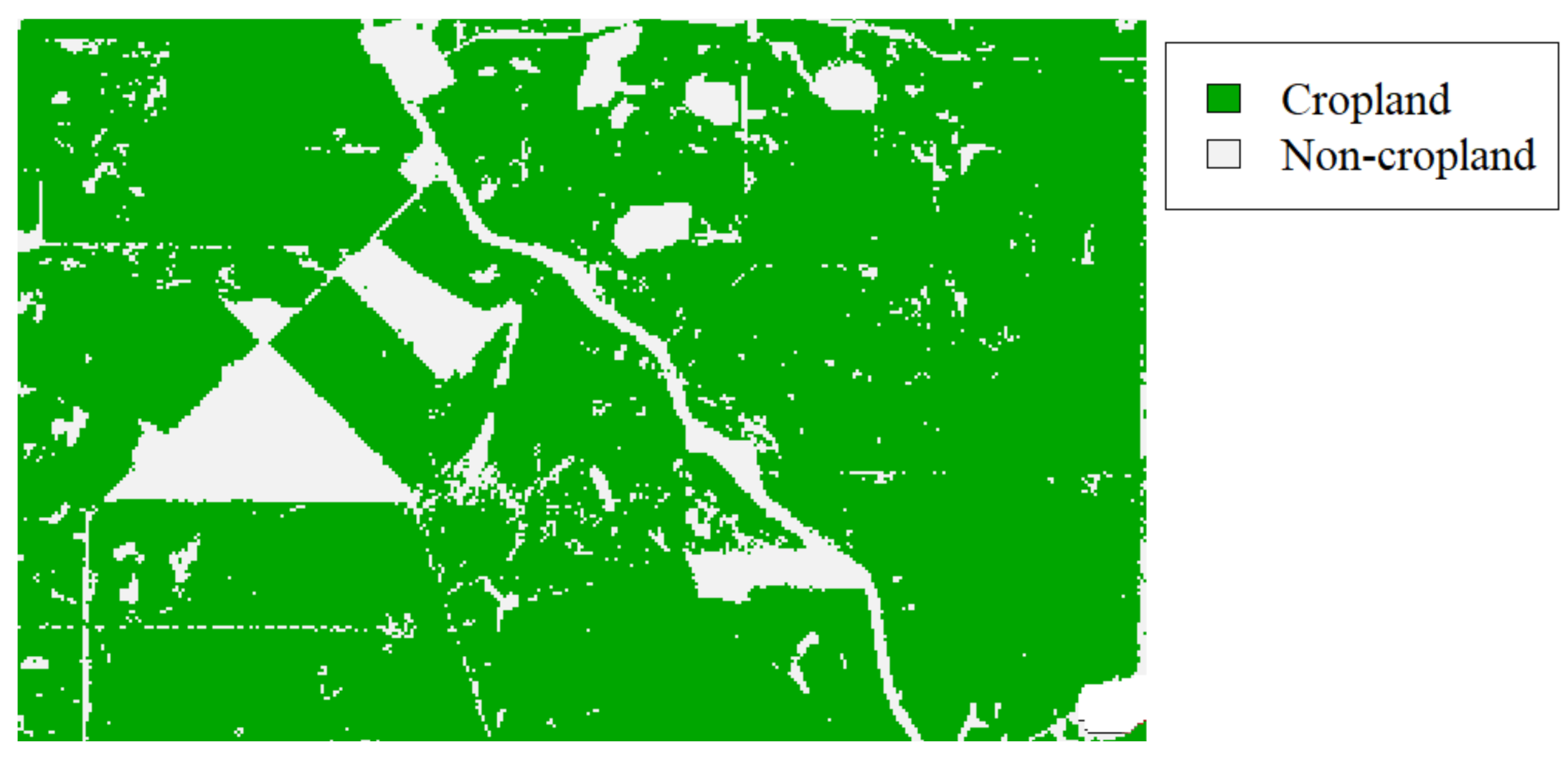
2.1.1. Study Area

The study area is located in the Western Australian grain belt at around 31.28 S and 118.16 E (Figure 1). It is approximately 8000 ha in size, which compares to an average farm size for the region of 5000 ha. Grain crops are grown in a dryland system that is heavily reliant on winter rainfall during the May to October growing season. Average growing season rainfall is between 200 and 300 mm. Wheat is the main crop grown, with barley, lupins, canola and pasture included in cropping rotations. As well as cropland, the study area includes areas of remnant vegetation (native trees and shrubs) and salt scalds caused by dryland salinity.

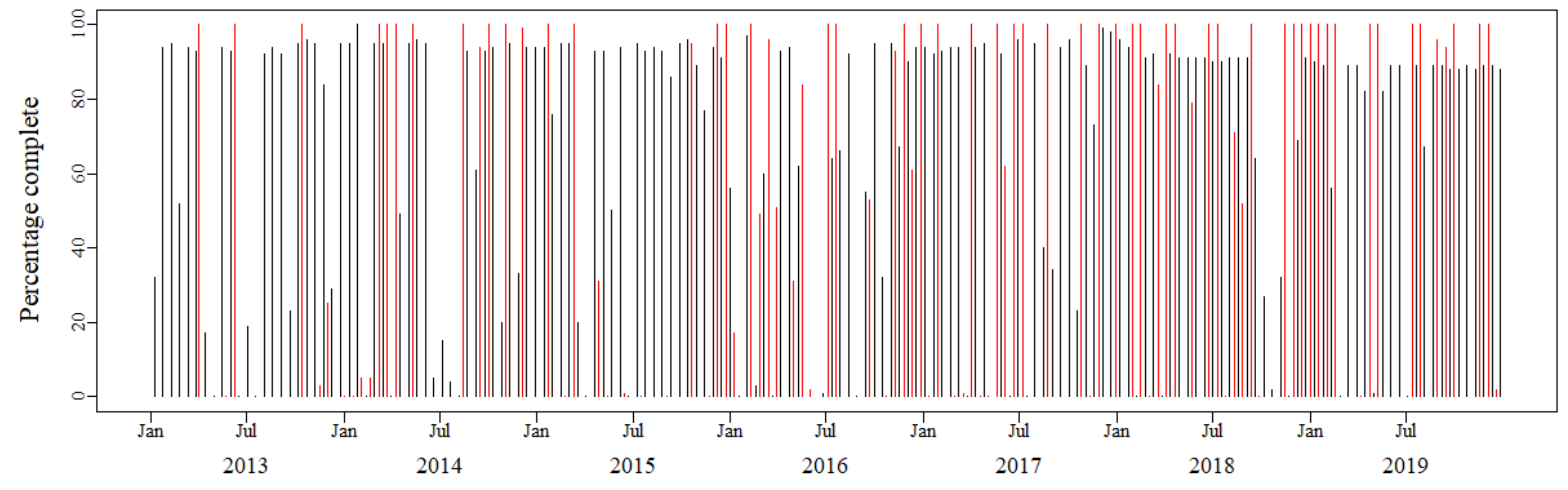
2.1.2. Landsat Data

All bands of Landsat-7 (path/row: 111/082) and Landsat-8 (path/row: 111/082) data from 2013 to 2019 were obtained from the United States Geological Survey (USGS) website (https://earthexplorer.usgs.gov accessed on 2 February 2021). There were 157 Landsat-7 images and 150 Landsat-8 images available during 2013 to 2019. Data preprocessing including geometric correction, top of atmosphere reflectance correction and surface reflectance correction were completed using the USGS Earth Resources Observation and Science (EROS) Centre Science Processing Architecture (ESPA) online interface (https://espa.cr.usgs.gov accessed on 2 February 2021). Cells with cloud contamination or cloud shadow were removed using the cell quality control band. The corrected red and near-infrared reflectances were used to calculate NDVI for all available image dates. Figure 2 shows the Landsat data coverage and percentage complete (i.e., the percentage area not affected by cloud, cloud shadow or the Landsat-7 SLC failure).

Due to reflective wavelength differences between the Landsat-7 and Landsat-8 sensors, Landsat-8 NDVI is typically greater than the Landsat-7 NDVI. Statistical functions can be used to transform one to the other [61]. Therefore, the observed Landsat-8 images are calibrated to adjust for differences between Landsat-7 and Landsat-8 NDVI using the method of Roy et al. [61] with an overlap region near the study site (Figure 3). The formula used to calibrate Landsat-8 NDVI observations to Landsat-7 NDVI is given by

$${\mathrm{NDVI}}_7=-0.02335149+0.92543372{ \mathrm{NDVI}}_8$$

(1)

2.2. Methods

2.2.1. Double-Lorentz Growth Curve

Crop growth was modelled using an asymmetric double-Lorentz function for the two main phases of crop development as measured by NDVI, which we refer to as the vegetative phase (from germination to maximum vegetative growth) and the grain-fill phase (from maximum growth to senescence). The curve takes the form

$$y=\left\{\begin{array}{ll}c+\left(d-c\right) / (1+b {\left(x-e\right)}^2,& x\le e\\ c+\left(d-c\right) / (1+b {\left(x-f\right)}^2,& x>e\end{array}\right.$$

(2)

where x is the day of year, $0\le c\le 0.9$ is the minimum NDVI, $0.1\le d\le 1$ is the maximum NDVI, $0\le e\le 260$ is the day of year at which maximum NDVI is observed, and b and f are the shape parameters for the curve before and after maximum NDVI is observed.

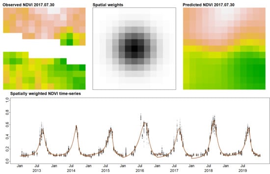
2.2.2. Spatially Weighted Phenology Detection

The SWGC method estimates asymmetric double-Lorentz growth curves for each year using data from a spatial neighbourhood around each cell, where the data are weighted according to distance from the central cell using a distance–decay kernel. Spatial weights are similarly used in GWR, and a range of distance weighting kernels are available [62]. To speed implementation, we investigated the specific case of a truncated or ‘moving window’ Gaussian kernel, where the distance weights are set to zero for all cells (x, y) outside of a rectangular region centred on the location for which the growth curve is being estimated, with size specified by MAXD such that the window has width and length equal to $\left(2\ast MAXD+1\right)$ m. Within the window, distance weights are given by

$$w_{x,y}=\exp \left(-\frac{1}{2}{\left(\frac{d_{x,y}}{b}\right)}^2\right)$$

(3)

where $w_{x,y}$ is the weight for cell (x, y), $d_{x,y}$ is the distance of (x, y) from the location for which the growth curve is to be estimated and b is the Gaussian kernel bandwidth.

Selection of appropriate values for b and MAXD will depend on the spatial resolution of the source data. Larger values of b will result in more spatially smooth estimates. To ensure filling of gaps in Landsat-7 data caused by the SLC failure, we chose kernel bandwidth b = 60 m and MAXD = 200 m. This kernel bandwidth ensures sufficient data with nonzero weights in the estimation of SLC failure gaps (Figure 4a). MAXD is chosen to be as small as possible while retaining all data with weights within three decimal places from zero (Figure 4b). Predictions obtained using these choices are spatially smoothed but not so much that they would not be useful at within-field scales (Figure 4c).

The SWGC method for spatially weighted estimation of continuous vegetation index sequences and within-field crop phenology was as applied to each cell using the following steps:

• Extract cells within the square MAXD window.
• Calculate distance-based weights for the extracted cells using a Gaussian kernel with bandwidth b.
• For each year:
  • Subset March to December data.
  • Estimate growth curve parameters for the cell and year using distance-based weights using nonlinear least-squares regression.
  • Use the estimated growth curve parameters to predict NDVI for any day of year.

2.2.3. Comparison of SWGC and Nonspatial Growth Curve Estimation

We compared SWGC with nonspatial growth curve estimation using an asymmetric double-Lorentz growth curve using a train/test approach. In all, 157 available Landsat-7 images between 2013 and 2019 were used to estimate growth curve parameters using the nonspatial and SWGC methods. Predictions were made for both the Landsat-7 training data and for the acquisition dates of the 150 available Landsat-8 images during the same time period. Of the 150 available Landsat-8 images, 95 were at least 80% cloud free. These were used as an independent test set to validate the accuracy of the SWGC method compared to nonspatial growth curve estimation using double-Lorentz growth curves. Accuracy was assessed using the Pearson correlation coefficient (correlation) between observed and predicted NDVI, root mean square error (RMSE) and mean absolute error (MAE), defined as follows:

$$\mathrm{Correlation}=\sqrt{1-\frac{{{\displaystyle \sum }}_{\mathrm{i}=1}^{\mathrm{n}}{\left({\mathrm{y}}_{\mathrm{i}}-{\hat{\mathrm{y}}}_{\mathrm{i}}\right)}^2}{{{\displaystyle \sum }}_{\mathrm{i}=1}^{\mathrm{n}}{\left({\mathrm{y}}_{\mathrm{i}}-\overline{\mathrm{y}}\right)}^2}}$$

(4)

$$\mathrm{MAE}=\frac{1}{n}{\displaystyle \sum }_{\mathrm{i}=1}^{\mathrm{n}}\left|{\mathrm{y}}_{\mathrm{i}}-{\hat{\mathrm{y}}}_{\mathrm{i}}\right|$$

(5)

$$\mathrm{RMSE}=\sqrt{\frac{1}{n}{\displaystyle \sum }_{\mathrm{i}=1}^{\mathrm{n}}{\left({\mathrm{y}}_{\mathrm{i}}-{\hat{\mathrm{y}}}_{\mathrm{i}}\right)}^2}$$

(6)

where ${\mathrm{y}}_{\mathrm{i}}$ are the observed NDVI values, $\overline{\mathrm{y}}$ is their mean and ${\hat{\mathrm{y}}}_{\mathrm{i}}$ are the predicted NDVIs.

We considered accuracy for the entire study area and for cropland only. The cropland mask was created by manually digitising 22 sites around the study area encompassing different land cover types: wheat crops, barley crops, canola crops, bare soil, remnant vegetation, salt-affected and roaded areas. The sites were used as training data for a random forest classifier using all bands of the Landsat-8 OLI image acquired on 29 August 2019 during the peak of the crop growing season. The random forest was used to classify the image into land cover classes that were then aggregated to form a binary mask for cropland, where cropland includes crops and bare soil (Figure 5).

2.2.4. SWGC Validation

To understand the performance of the SWGC method for spatially weighted growth curve estimation, we performed further validation that considers accuracy for individual cells (per-cell accuracy) and individual images (per-image accuracy). Our aim in validation was to communicate when SWGC works well, when it does not and why it can fail.

Per-cell accuracy was calculated by extracting observed and predicted NDVI for each cell in the Landsat-8 test data sequence and calculating the correlation, MAE and RMSE. Each of the three accuracy statistics was mapped to show where accuracy is high and low. To demonstrate how spatial weights are used in the estimation of growth curves for different locations, weighted data and estimated growth curves are shown for selected cells from within the study area.

Per-image accuracy was calculated by extracting observed and predicted NDVI for each image in the Landsat-8 test data sequence and calculating the correlation, MAE and RMSE for both the entire study area and for cropland only. We considered how the accuracy varies throughout the year by considering the accuracy for each month. To show when and where errors occur in any one image, we selected three Landsat-8 images during the growing season: two with lower accuracy than typically found and one with more-typical SWGC accuracy. For these three images, we show: (a) the observed Landsat-8 NDVI; (b) SWGC predicted NDVI; (c) the scatterplot of observed versus predicted NDVI coloured by density and (d) a time-series plot showing the weighted Landsat-7 NDVI data used in SWGC estimation, the observed Landsat-8 NDVI data and the estimated growth curve. Results for all images, including maps of observed and predicted NDVI and scatterplots (coloured by density) of observed versus predicted NDVI are included in Supplementary Materials 1 for the Landsat-7 training data and Supplementary Materials 2 for the Landsat-8 test data. Supplementary Materials 1 includes instances when cloud cover affected most or all of the image. Supplementary Materials 2 only shows results for images that were more than 80% cloud free.

3. Results

3.1. Comparison of SWGC and Nonspatial Growth Curve Estimation

Table 1. Average accuracy of nonspatial growth curve and SWGC methods for NDVI prediction for the Landsat-8 test data.

	Method	Correlation	MAE	RMSE
Study area	Nonspatial	0.534	0.048	0.211
Cropland only	Nonspatial	0.601	0.042	0.194
Study area	SWGC	0.932	0.033	0.053
Cropland only	SWGC	0.952	0.027	0.047

shows the overall accuracy of predicting NDVI for each cell in the 95-image Landsat-8 test data set using nonspatial growth curve estimation and SWGC. Statistics are reported for the entire study area and for cropland only. Because both the spatial and nonspatial methods constrain temporal predictions by use of the growth curve, both methods have higher accuracy for cropland areas. SWGC results in more accurate per-cell predictions for both the study area and cropland. For the entire study area, SWGC improves the correlation by 75%, MAE by 31% and RMSE by 75%. For cropland, the correlation is improved by 58%, the MAE by 36% and the RMSE by 76%.

3.2. SWGC Validation

3.2.1. Per-Cell Accuracy

Figure 6 maps the per-cell accuracy of the SWGC method. Areas with high RMSE but not necessarily high MAE have greater NDVI variability, such as lower-yielding cropland. Accuracy is highest for cropland, which has higher correlation and lower RMSE than noncropland areas that include remnant vegetation, which has greater NDVI variability, and for bare or salt-affected areas, dams, roads and paddock boundaries that do not experience annual green-up and brown-off cycles.

Figure 7 shows the fitted response curves for four cells in the study area. Figure 7a shows the fitted response curve and data for a typical remnant vegetation cell with higher error. The NDVI data (both the Landsat-7 and Landsat-8) are noisier, and the seasonal signal of the NDVI has smaller amplitude and a larger wavelength with green-up beginning earlier and brown-off later than for cropland. In contrast, Figure 7b shows a typical cropland cell with low error. Green-up tends to occur around June/July and brown-off at around the end of October. The growth curve amplitude varies from season to season depending on the type of crop grown and seasonal rainfall. Figure 7c shows a cropland cell with poorer accuracy. Because the growth curves are estimated independently for each year, there can be a mismatch at the start of the year as seen here. Years 2013 and 2014 appear to fit the data reasonably well, despite missing data in the Landsat-7 training set in the early part of the growing season.

However, the SWGC method performed poorly in 2016. This is due to a combination of missing data early in the growing season and because the Landsat-7 cell quality control band did not adequately detect cloud in the image acquired on 2016-07-19 (see Supplementary Materials 2). This resulted in underprediction of NDVI prior to maximum greenness. In years 2018 and 2019, there appears to be NDVI variability in the combined Landsat-7 and Landsat-8 sequence that leads to less-accurate predictions of Landsat-8 NDVI. Figure 7d shows that for 2014 and 2017, SWGC can predict a higher peak of season NDVI than is evident in the data.

3.2.2. Per-Image Accuracy

Detailed results including images and scatterplots (coloured by density) of observed and predicted NDVI are included in Supplementary Materials 1 for the Landsat-7 training data and in Supplementary Materials 2 for the Landsat-8 test data. Supplementary Materials 1 includes instances when cloud cover affected most or all of the image. Supplementary Materials 2 only shows results for images that were more than 80% cloud free. This section summarises the results for the Landsat-8 test data.

Figure 8 shows the correlation, MAE and RMSE between observed and predicted NDVI for each image in the Landsat-8 test data for the entire study area and for cropland only. Per-image correlation ranged from 0.29 to 0.90, with a mean of 0.79. Per-image cropland correlation was higher, ranging from 0.29 to 0.98, with a mean of 0.91. MAE and RMSE were similar for cropped and non-cropped areas, with mean MAE of 0.03 and mean RMSE of 0.04.

Figure 9 shows monthly accuracy statistics. Per-image MAE and RMSE are higher in winter months because of higher greenness, but the months from July to September have the highest correlations. MAE and RMSE are similar in winter, meaning there are few errors caused by large outliers. However, summer RMSE is higher than MAE meaning there are likely high observed NDVI outliers.

Errors in any one image occur when there are too many missing cloud-free images in the NDVI sequence. For example, in 2014 there were no Landsat-7 images available from June to mid-August. As a result, SWGC failed to adequately estimate maximum NDVI for some cells. This is shown in Figure 10. Compared to the observed NDVI for 2014-08-15 (Figure 10a), the predicted NDVI (Figure 10b) was too high during the season’s peak in some areas, as shown in Figure 10c. Figure 10d shows the time series of observed and predicted data for a typical cell where this occurred. The full dynamics of the NDVI time-sequence can be seen in Supplementary Materials 2.

As noted in Section 3.2.1, SWGC performs poorly in 2016 because of a combination of missing data early in the growing season and inadequate cloud-masking for the image acquired on 2016-07-19. Figure 11 shows the effect on the 2016-07-03 prediction, where the observed NDVI (Figure 11a) is lower than the predicted NDVI (Figure 11b) for the eastern part of the image. This can be seen in the scatterplot of observed versus predicted NDVI for the image (Figure 11c). The time-series for a cell in the affected area (Figure 11d) shows how the early season missing data and low observed NDVI that was not flagged as being cloud-affected (and therefore masked out) on 2016-07-19 affect the growth curve estimation.

Figure 12 shows more typical results for a winter image acquired on 2018-07-25 with observed NDVI shown in Figure 12a, predicted NDVI in Figure 12b, scatterplot of observed versus predicted NDVI in Figure 12c and the time-series for a cropland cell shown in Figure 12d.

4. Discussion

In this study, we developed a new method for the estimation of continuous sequences of VIs that uses spatially weighted data from a neighbourhood around each cell in the estimation of crop growth curves. The SWGC method was designed specifically for Landsat data to generate long-term records of grain crop growth to assist precision agriculture decision-making in Mediterranean environments, but it could be applied to VIs derived from any remote source. It differs from other methods for gap-filling Landsat data in that it does not require fusion with data from satellites with more frequent revisit times or finer spatial resolution. Using only Landsat data, it fills gaps caused by the Landsat-7 SLC failure and cloud and adequately captures peak of season NDVI despite frequent cloud occurrence during winter when crops reach maximum growth.

We tested SWGC using an independent data set, where all 157 available Landsat-7 images between 2013 and 2019 were used to train the model, and 95 Landsat-8 images from the same period that were at least 80% cloud free were used to test its performance. Our results show that use of spatially weighted data in crop growth curve estimation improves the estimation of continuous Landsat NDVI sequences. The combined use of an asymmetric double-Lorentz growth curve and spatially weighted data allow estimates of peak of season NDVI that are higher than observed NDVI values. Because the growth curve was chosen to capture winter crop growth, SWGC as we have implemented it performs better for cropland than for non-crop areas, but accuracy statistics for the entire study area are still good. Using a 7-year data record, the only major errors occurred when cloud-affected Landsat-7 data in 2016 were not flagged as cloudy and removed from the training data. In years 2013 and 2014, scenes were missing during the vegetative phase of the growing season with no complete Landsat-7 scene in June or July in 2013, and there were four missing consecutive scenes between July and August in 2014. Despite this, there was only one Landsat-8 scene in those periods for which the test data accuracy was poorer and that was a scene with only a small area that was not cloud-affected, which resulted in biases toward lower scene-average correlation and higher scene-average MAE and RMSE. Thus, SWGC can correct for continuously and frequently missing data in the NDVI training set, except in cases where cloud removal is not adequately performed prior to analysis.

SWGC accuracy (correlation = 0.932, MAE = 0.033, RMSE = 0.053 overall and correlation = 0.952, MAE = 0.027, RSE = 0.047 for cropland) can be compared with other published methods for gap-filling Landsat data. Zhu et al. [20] used harmonic time-series for each cell to fill gaps in Landsat sequences and reported RMSEs of 0.01 to 0.02 for visible bands and 0.02 to 0.03 for the near-infrared band, which would correspond to a slightly lower RMSE for the NDVI than we found using SWGC (RMSE = 0.053). However, their validation is biased because they reported accuracy statistics calculated using the same data that were used to train the models rather than an independent data set, and therefore their statistics do not capture the ability to fill actual data gaps. Roy and Yan [46] also used harmonic models with Landsat data. To compare different model forms, they estimated accuracy using root mean square difference (RMSD), which takes the number of model parameters into account. Histograms for six regions showed similar or higher values than SWGC RMSE for cropland.

SWGC can also be compared to methods for gap-filling that fuse Landsat with MODIS data. Walker et al. [24] used the STARFM [27] algorithm and tested its performance using 5% of vegetated cells from 10 images acquired in 2006 and 2009, which were the same image used as reference images to train the STARFM algorithm. They calculated the median correlation between observed and actual reflectances, which ranged from 0.521 to 0.945 with a median of 0.70, compared to the SWGC mean correlation of 0.952 between observed and predicted NDVI. Gao et al. [23] similarly used STARFM to estimate phenology from Landsat-MODIS fusion using data from 2001 to 2014. They omitted Landsat images with missing data and years with insufficient images from the data fusion process and used non-cloud cells from incomplete scenes to assess the estimation of NDVI from the fused data set. They reported a correlation of 0.918 between observed and predicted NDVI, with MAE of 0.072 and RMSE of 0.100, which compares with SWGC results of 0.952, 0.027 and 0.047for correlation, MAE and RMSE, respectively. Zhou and Zhong [25] presented a Kalman filter approach for generating synthetic time-series of fused Landsat and MODIS images for 2016, with correlations for visible bands ranging from 0.921 to 0.96 and for the near-infrared band 0.960 to 0.939. RMSE ranged from 0.007 to 0.015 for visible bands and from 0.023 to 0.032 for the near-infrared band. This corresponds to similar correlation for NDVI prediction and slightly lower MAE and RMSE than we found for SWGC.

The main limitation of the SWGC method is that predictions are spatially smoothed. Our use of a Gaussian kernel with a 60 m bandwidth resulted in visible smoothing where lineal features one cell wide (such as roads and paddock boundaries) can lose definition and spatial variability in fields is also reduced. This means that SWGC estimates are less precise than methods for gap-filling that fuse Landsat with MODIS data, and they will not be as useful for applications that require fine-scale estimates. However, our goal is to produce long-term, medium-resolution records to understand the climate–crop dynamics of broadacre grain cropping systems and support on-farm decision-making. Are spatially smoothed estimates useful for this purpose? We assert that they are because (1) field size is large; and (2) most decisions about in-field crop management are currently based on interpolated yield maps that have been substantially smoothed. Of course, the degree of smoothing by SWGC is determined by the choice of smoothing kernel and its bandwidth, and these choices can be adapted for different uses. This makes the SWGC algorithm adaptable. While it may not be useful in highly heterogenous landscapes, it can potentially be used for other landcover monitoring, such as pastures, grassland, forestry and wetlands. We developed SWGC for use with Landsat NDVI data for long-term, within-field crop monitoring. However, it can be applied to any VI from any remotely sensed source and using any method of growth curve estimation.

So that the Landsat-8 data could be retained for use as an independent test set, we only used Landsat-7 data to train SWGC in this study. We tested SWGC using a relatively small study area located in a dryland cropping region with low rainfall. It is likely that the percentage completeness of the Landsat-7 training data within the growing season was higher for our study area than for other areas with more rainfall and more rainy days. For this reason, it may be difficult to apply SWGC in different areas and achieve the levels of accuracy we report. Many studies have demonstrated better results for LSP detection when using a higher frequency of observations [34,52,63]. We expect the SWGC method will have better performance when combined Landsat-5, Landsat-7 and Landsat-8 data are used and recommend combined data sets be used as best practice to take full advantage of the Landsat series data. However, there may still be instances when there are insufficient cloud-free images for SWGC to be applied in some locations and growing seasons.

SWGC is a simple approach that is more computationally efficient than most methods requiring fusion of data from multiple sources. Its novelty lies in the incorporation of spatial weights into crop growth curve estimation to gap-fill Landsat images and produce long-term, complete sequences of Landsat NDVI. We envisage two main ways that the SWGC method can be improved to reduce spatial smoothing of predicted sequences of NDVI. First, a local geostatistical approach could be used to vary the spatial weights by location according to local autocorrelation calculated using the empirical semivariogram [64]. Second, a land cover classification could be employed to ensure only weights from neighbouring cells with the same land cover are used as used by [15,16]. Our proposed improvements would still differ from other geostatistical gap-filling methods by using crop growth curves rather than linear kriging.

5. Conclusions

We conclude that incorporating spatial weights according to geographic distance in the estimation of crop growth curves can improve the estimation of continuous sequences of NDVI from Landsat data. This allows the generation of long-term sequences to develop a better understanding of how crop growth varies in space and time according to soil types, local weather conditions, seasonal climate variability and management to support decision-making about how to optimise crop management within fields.

References

- Robert, P.C. Precision agriculture: A challenge for crop nutrition management. Plant Soil 2002, 247, 143–149. [Google Scholar] [CrossRef]
- Chen, K.; O’Leary, R.A.; Evans, F.H. A simple and parsimonious generalised additive model for predicting wheat yield in a decision support tool. Agric. Syst. 2019, 173, 140–150. [Google Scholar] [CrossRef]
- Bramley, R.G.V.; Ouzman, J. Farmer attitudes to the use of sensors and automation in fertilizer decision-making: Nitrogen fertilization in the Australian grains sector. Precis. Agric. 2019, 20, 157–175. [Google Scholar] [CrossRef]
- Rouse, J.W.; Haas, R.H.; Schell, J.A.; Deering, D.W. Monitoring Vegetation Systems in the Great Plains with ERTS. In Proceedings of the 3rd ERTS-1 Symposium held by Goddard Space Flight Center, Washington, DC, USA, 10–14 December 1973; pp. 309–317. [Google Scholar]
- Huete, A.; Didan, K.; Miura, T.; Rodriguez, E.P.; Gao, X.; Ferreira, L.G. Overview of the radiometric and biophysical performance of the MODIS vegetation indices. Remote Sens. Environ. 2002, 83, 195–213. [Google Scholar] [CrossRef]
- Sakamoto, T.; Wardlow, B.D.; Gitelson, A.A.; Verma, S.B.; Suyker, A.E.; Arkebauer, T.J. A Two-Step Filtering approach for detecting maize and soybean phenology with time-series MODIS data. Remote Sens. Environ. 2010, 114, 2146–2159. [Google Scholar] [CrossRef]
- Zeng, L.; Wardlow, B.D.; Xiang, D.; Hu, S.; Li, D. A review of vegetation phenological metrics extraction using time-series, multispectral satellite data. Remote Sens. Environ. 2020, 237. [Google Scholar] [CrossRef]
- de Beurs, K.M.; Henebry, G.M. Spatio-Temporal Statistical Methods for Modelling Land Surface Phenology. In Phenological Research; Hudson, I.L., Keatley, M.R., Eds.; Springer: Dordrecht, The Netherlands, 2010; pp. 177–208. [Google Scholar] [CrossRef]
- Belward, A.S.; Skøien, J.O. Who launched what, when and why; trends in global land-cover observation capacity from civilian earth observation satellites. Isprs J. Photogramm. Remote Sens. 2015, 103, 115–128. [Google Scholar] [CrossRef]
- Irons, J.R.; Dwyer, J.L.; Barsi, J.A. The next Landsat satellite: The Landsat Data Continuity Mission. Remote Sens. Environ. 2012, 122, 11–21. [Google Scholar] [CrossRef] [Green Version]
- Wulder, M.A.; Loveland, T.R.; Roy, D.P.; Crawford, C.J.; Masek, J.G.; Woodcock, C.E.; Allen, R.G.; Anderson, M.C.; Belward, A.S.; Cohen, W.B.; et al. Current status of Landsat program, science, and applications. Remote Sens. Environ. 2019, 225, 127–147. [Google Scholar] [CrossRef]
- Wulder, M.A.; Masek, J.G.; Cohen, W.B.; Loveland, T.R.; Woodcock, C.E. Opening the archive: How free data has enabled the science and monitoring promise of Landsat. Remote Sens. Environ. 2012, 122, 2–10. [Google Scholar] [CrossRef]
- Whitcraft, A.K.; Vermote, E.F.; Becker-Reshef, I.; Justice, C.O. Cloud cover throughout the agricultural growing season: Impacts on passive optical earth observations. Remote Sens. Environ. 2015, 156, 438–447. [Google Scholar] [CrossRef]
- Scaramuzza, P. SLC Gap-Filled Products Phase One Methodology; USGS: Sioux Falls, SD, USA, 2004.
- Chen, J.; Zhu, X.; Vogelmann, J.E.; Gao, F.; Jin, S. A simple and effective method for filling gaps in Landsat ETM+ SLC-off images. Remote Sens. Environ. 2011, 115, 1053–1064. [Google Scholar] [CrossRef]
- Zhu, X.; Liu, D.; Chen, J. A new geostatistical approach for filling gaps in Landsat ETM+ SLC-off images. Remote Sens. Environ. 2012, 124, 49–60. [Google Scholar] [CrossRef]
- Wang, Q.; Wang, L.; Li, Z.; Tong, X.; Atkinson, P.M. Spatial-Spectral Radial Basis Function-Based Interpolation for Landsat ETM+ SLC-Off Image Gap Filling. IEEE Trans. Geosci. Remote Sens. 2020, 1–17. [Google Scholar] [CrossRef]
- Maxwell, S.K.; Schmidt, G.L.; Storey, J.C. A multi-scale segmentation approach to filling gaps in Landsat ETM+ SLC-off images. Int. J. Remote Sens. 2007, 28, 5339–5356. [Google Scholar] [CrossRef]
- Salman, S.S. Adaptive Method for Landsat ETM+ Gap Filling Using Successive Temporal Images. NeuroQuantology 2020, 18, 112–122. [Google Scholar] [CrossRef]
- Zhu, Z.; Woodcock, C.E.; Holden, C.; Yang, Z. Generating synthetic Landsat images based on all available Landsat data: Predicting Landsat surface reflectance at any given time. Remote Sens. Environ. 2015, 162, 67–83. [Google Scholar] [CrossRef]
- Azzari, G.; Jain, M.; Lobell, D.B. Towards fine resolution global maps of crop yields: Testing multiple methods and satellites in three countries. Remote Sens. Environ. 2017, 202, 129–141. [Google Scholar] [CrossRef]
- Kang, Y.; Özdoğan, M. Field-level crop yield mapping with Landsat using a hierarchical data assimilation approach. Remote Sens. Environ. 2019, 228, 144–163. [Google Scholar] [CrossRef]
- Gao, F.; Anderson, M.C.; Zhang, X.; Yang, Z.; Alfieri, J.G.; Kustas, W.P.; Mueller, R.; Johnson, D.M.; Prueger, J.H. Toward mapping crop progress at field scales through fusion of Landsat and MODIS imagery. Remote Sens. Environ. 2017, 188, 9–25. [Google Scholar] [CrossRef] [Green Version]
- Walker, J.J.; de Beurs, K.M.; Wynne, R.H. Dryland vegetation phenology across an elevation gradient in Arizona, USA, investigated with fused MODIS and Landsat data. Remote Sens. Environ. 2014, 144, 85–97. [Google Scholar] [CrossRef]
- Zhou, F.; Zhong, D. Kalman filter method for generating time-series synthetic Landsat images and their uncertainty from Landsat and MODIS observations. Remote Sens. Environ. 2020, 239, 111628. [Google Scholar] [CrossRef]
- Sedano, F.; Kempeneers, P.; Hurtt, G. A Kalman Filter-Based Method to Generate Continuous Time Series of Medium-Resolution NDVI Images. Remote Sens. 2014, 6, 12381–12408. [Google Scholar] [CrossRef] [Green Version]
- Gao, F.; Masek, J.; Schwaller, M.; Hall, F. On the blending of the Landsat and MODIS surface reflectance: Predicting daily Landsat surface reflectance. IEEE Trans. Geosci. Remote Sens. 2006, 44, 2207–2218. [Google Scholar] [CrossRef]
- Zhu, X.; Chen, J.; Gao, F.; Chen, X.; Masek, J.G. An enhanced spatial and temporal adaptive reflectance fusion model for complex heterogeneous regions. Remote Sens. Environ. 2010, 114, 2610–2623. [Google Scholar] [CrossRef]
- Bolton, D.K.; Gray, J.M.; Melaas, E.K.; Moon, M.; Eklundh, L.; Friedl, M.A. Continental-scale land surface phenology from harmonized Landsat 8 and Sentinel-2 imagery. Remote Sens. Environ. 2020, 240, 111685. [Google Scholar] [CrossRef]
- Houborg, R.; McCabe, M.F. A Cubesat enabled Spatio-Temporal Enhancement Method (CESTEM) utilizing Planet, Landsat and MODIS data. Remote Sens. Environ. 2018, 209, 211–226. [Google Scholar] [CrossRef]
- Broich, M.; Huete, A.; Paget, M.; Ma, X.; Tulbure, M.; Coupe, N.R.; Evans, B.; Beringer, J.; Devadas, R.; Davies, K.; et al. A spatially explicit land surface phenology data product for science, monitoring and natural resources management applications. Environ. Model. Softw. 2015, 64, 191–204. [Google Scholar] [CrossRef]
- Kong, D.; Zhang, Y.; Gu, X.; Wang, D. A robust method for reconstructing global MODIS EVI time series on the Google Earth Engine. Isprs J. Photogramm. Remote Sens. 2019, 155, 13–24. [Google Scholar] [CrossRef]
- Jönsson, P.; Eklundh, L. TIMESAT—A program for analyzing time-series of satellite sensor data. Comput. Geosci. 2004, 30, 833–845. [Google Scholar] [CrossRef] [Green Version]
- Cao, R.; Chen, Y.; Shen, M.; Chen, J.; Zhou, J.; Wang, C.; Yang, W. A simple method to improve the quality of NDVI time-series data by integrating spatiotemporal information with the Savitzky-Golay filter. Remote Sens. Environ. 2018, 217, 244–257. [Google Scholar] [CrossRef]
- Araya, S.; Ostendorf, B.; Lyle, G.; Lewis, M. Remote sensing derived phenological metrics to assess the spatio-temporal growth variability in cropping fields. Adv. Remote Sens. 2017, 6, 212–228. [Google Scholar] [CrossRef] [Green Version]
- Araya, S.; Ostendorf, B.; Lyle, G.; Lewis, M. CropPhenology: An R package for extracting crop phenology from time series remotely sensed vegetation index imagery. Ecol. Inform. 2018, 46, 45–56. [Google Scholar] [CrossRef]
- Elmore, A.J.; Guinn, S.M.; Minsley, B.J.; Richardson, A.D. Landscape controls on the timing of spring, autumn, and growing season length in mid-Atlantic forests. Glob. Chang. Biol. 2012, 18, 656–674. [Google Scholar] [CrossRef] [Green Version]
- Beck, P.S.A.; Atzberger, C.; Høgda, K.A.; Johansen, B.; Skidmore, A.K. Improved monitoring of vegetation dynamics at very high latitudes: A new method using MODIS NDVI. Remote Sens. Environ. 2006, 100, 321–334. [Google Scholar] [CrossRef]
- Fisher, J.; Mustard, J.; Vadeboncoeur, M. Green leaf phenology at Landsat resolution: Scaling from the field to the satellite. Remote Sens. Environ. 2006, 100, 265–279. [Google Scholar] [CrossRef]
- Zhao, H.; Yang, Z.; Di, L.; Pei, Z. Evaluation of Temporal Resolution Effect in Remote Sensing Based Crop Phenology Detection Studies. In Computer and Computing Technologies in Agriculture V; Springer: Berlin/Heidelberg, Germany, 2012; pp. 135–150. [Google Scholar] [CrossRef] [Green Version]
- Zhang, X.; Friedl, M.A.; Schaaf, C.B.; Strahler, A.H.; Hodges, J.C.F.; Gao, F.; Reed, B.C.; Huete, A. Monitoring vegetation phenology using MODIS. Remote Sens. Environ. 2003, 84, 471–475. [Google Scholar] [CrossRef]
- Zhang, X. Reconstruction of a complete global time series of daily vegetation index trajectory from long-term AVHRR data. Remote Sens. Environ. 2015, 156, 457–472. [Google Scholar] [CrossRef]
- Cao, R.; Chen, J.; Shen, M.; Tang, Y. An improved logistic method for detecting spring vegetation phenology in grasslands from MODIS EVI time-series data. Agric. For. Meteorol. 2015, 200, 9–20. [Google Scholar] [CrossRef]
- Wang, S.; Di Tommaso, S.; Deines, J.M.; Lobell, D.B. Mapping twenty years of corn and soybean across the US Midwest using the Landsat archive. Sci. Data 2020, 7, 307. [Google Scholar] [CrossRef]
- Ghaderpour, E.; Ben Abbes, A.; Rhif, M.; Pagiatakis, S.D.; Farah, I.R. Non-stationary and unequally spaced NDVI time series analyses by the LSWAVE software. Int. J. Remote Sens. 2019, 41, 2374–2390. [Google Scholar] [CrossRef]
- Roy, D.P.; Yan, L. Robust Landsat-based crop time series modelling. Remote Sens. Environ. 2020, 238, 110810. [Google Scholar] [CrossRef]
- Zeng, L.; Wardlow, B.D.; Wang, R.; Shan, J.; Tadesse, T.; Hayes, M.J.; Li, D. A hybrid approach for detecting corn and soybean phenology with time-series MODIS data. Remote Sens. Environ. 2016, 181, 237–250. [Google Scholar] [CrossRef]
- Zhou, M.; Ma, X.; Wang, K.; Cheng, T.; Tian, Y.; Wang, J.; Zhu, Y.; Hu, Y.; Niu, Q.; Gui, L.; et al. Detection of phenology using an improved shape model on time-series vegetation index in wheat. Comput. Electron. Agric. 2020, 173, 105398. [Google Scholar] [CrossRef]
- Sakamoto, T. Refined shape model fitting methods for detecting various types of phenological information on major U.S. crops. Isprs J. Photogramm. Remote Sens. 2018, 138, 176–192. [Google Scholar] [CrossRef]
- Kowalski, K.; Senf, C.; Hostert, P.; Pflugmacher, D. Characterizing spring phenology of temperate broadleaf forests using Landsat and Sentinel-2 time series. Int. J. Appl. Earth Obs. Geoinf. 2020, 92, 102172. [Google Scholar] [CrossRef]
- Zhang, Y.; Hepner, G.F. Short-Term Phenological Predictions of Vegetation Abundance Using Multivariate Adaptive Regression Splines in the Upper Colorado River Basin. Earth Interact. 2017, 21, 4644–4671. [Google Scholar] [CrossRef]
- Younes, N.; Joyce, K.E.; Maier, S.W. All models of satellite-derived phenology are wrong, but some are useful: A case study from northern Australia. Int. J. Appl. Earth Obs. Geoinf. 2021, 97, 102285. [Google Scholar] [CrossRef]
- Horton, W.S. An examination of five preferred orientation functions. Carbon 1979, 17, 153–155. [Google Scholar] [CrossRef]
- Brunsdon, C.; Fotheringham, S.; Charlton, M. Geographically weighted regression: A method for exploring spatial nonstationarity. Geogr. Anal. 1996, 28, 281–298. [Google Scholar] [CrossRef]
- Brunsdon, C.; Fotheringham, S.; Charlton, M. Geographically weighted regression—Modelling spatial non-stationarity. J. R. Stat. Soc. Ser. D (Stat.) 1998, 47, 431–443. [Google Scholar] [CrossRef]
- Fotheringham, S.; Brunsdon, C.; Charlton, M. Geographically Weighted Regression: The Analysis of Spatially Varying Relationships; Wiley: Chichester, UK, 2002. [Google Scholar]
- Gao, F.; Morisette, J.T.; Wolfe, R.E.; Ederer, G.; Pedelty, J.; Masuoka, E.; Myneni, R.; Tan, B.; Nightingale, J. An Algorithm to Produce Temporally and Spatially Continuous MODIS-LAI Time Series. IEEE Geosci. Remote Sens. Lett. 2008, 5, 60–64. [Google Scholar] [CrossRef]
- Tan, B.; Morisette, J.T.; Wolfe, R.E.; Gao, F.; Ederer, G.A.; Nightingale, J.; Pedelty, J.A. An Enhanced TIMESAT Algorithm for Estimating Vegetation Phenology Metrics From MODIS Data. IEEE J. Sel. Top. Appl. Earth Obs. Remote Sens. 2011, 4, 361–371. [Google Scholar] [CrossRef]
- Kiiveri, H.T.; Campbell, N.A. Allocation of remotely sensed data using Markov models for image data and pixel labels. Aust. J. Stat. 1992, 34, 361–374. [Google Scholar] [CrossRef]
- Cai, Y.; Guan, K.; Lobell, D.; Potgieter, A.B.; Wang, S.; Peng, J.; Xu, T.; Asseng, S.; Zhang, Y.; You, L.; et al. Integrating satellite and climate data to predict wheat yield in Australia using machine learning approaches. Agric. For. Meteorol. 2019, 274, 144–159. [Google Scholar] [CrossRef]
- Roy, D.P.; Kovalskyy, V.; Zhang, H.K.; Vermote, E.F.; Yan, L.; Kumar, S.S.; Egorov, A. Characterization of Landsat-7 to Landsat-8 reflective wavelength and normalized difference vegetation index continuity. Remote Sens. Environ. 2016, 185, 57–70. [Google Scholar] [CrossRef] [Green Version]
- Evans, F.H.; Recalde Salas, A.; Rakshit, S.; Scanlan, C.A.; Cook, S.E. Assessment of the use of geographically weighted regression for analysis of large on-farm experiments and implications for practical application. Agronomy 2020, 10, 1720. [Google Scholar] [CrossRef]
- Zhou, Q.; Rover, J.; Brown, J.; Worstell, B.; Howard, D.; Wu, Z.; Gallant, A.; Rundquist, B.; Burke, M. Monitoring Landscape Dynamics in Central U.S. Grasslands with Harmonized Landsat-8 and Sentinel-2 Time Series Data. Remote Sens. 2019, 11, 328. [Google Scholar] [CrossRef] [Green Version]
- Diggle, P.J.; Tawn, J.A. Model-based geostatistics. Appl. Stat. 1998, 47, 299–350. [Google Scholar] [CrossRef]