Evaluation of Object-Based Greenhouse Mapping Using WorldView-3 VNIR and SWIR Data: A Case Study from Almería (Spain)
Abstract
1. Introduction
2. Study Area
3. Datasets and Pre-Processing
3.1. WorldView-3 Image
3.2. Ground Truth
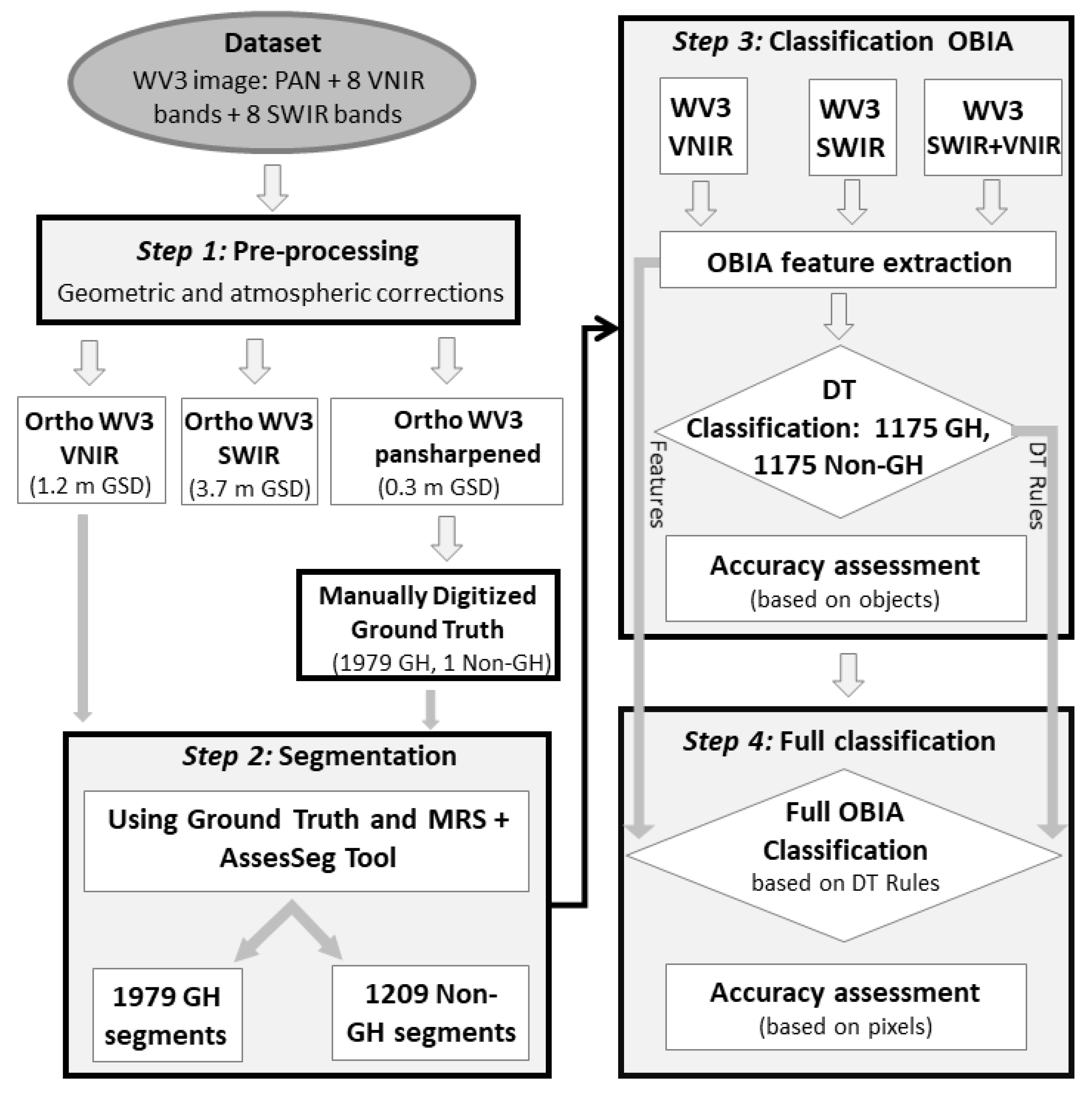
4. Methodology
4.1. Segmentation
4.2. Definition and Extraction of Object-Based Features
4.3. Decision Tree Modeling and Classification Accuracy Assessment
5. Results
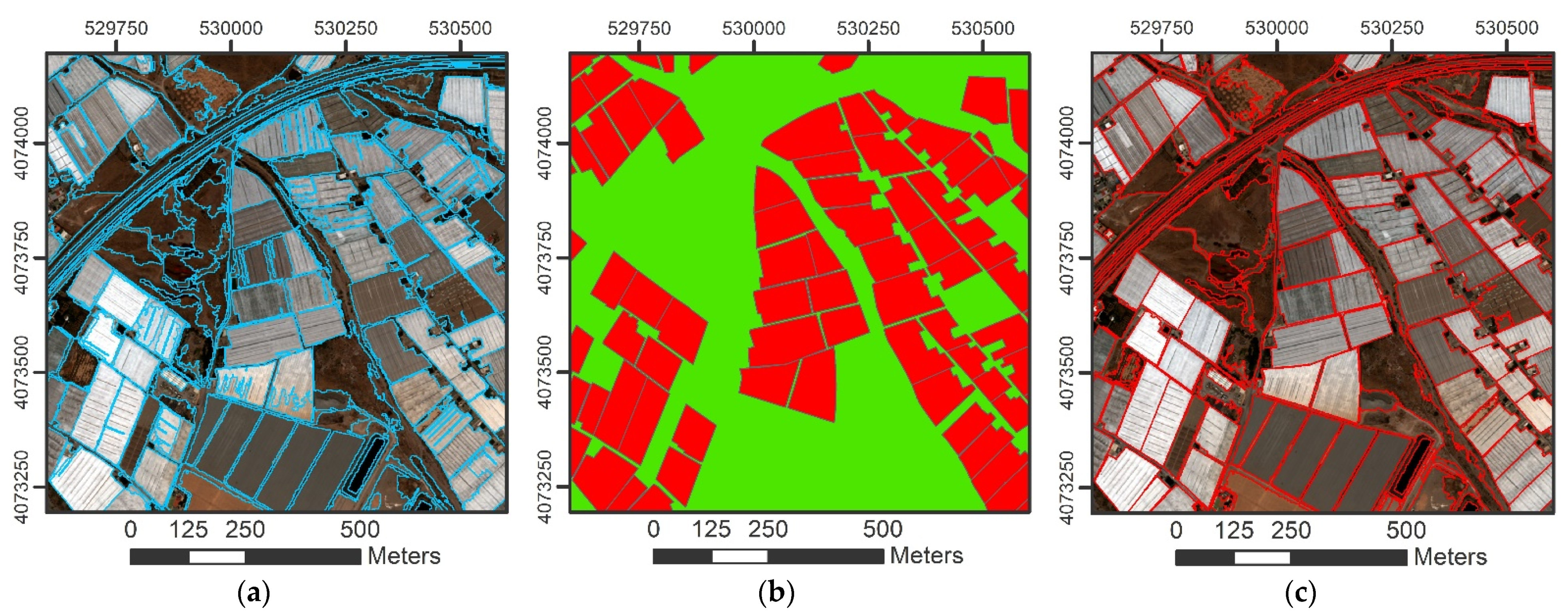
5.1. Segmentation
5.2. Object-Based Accuracy Assessment
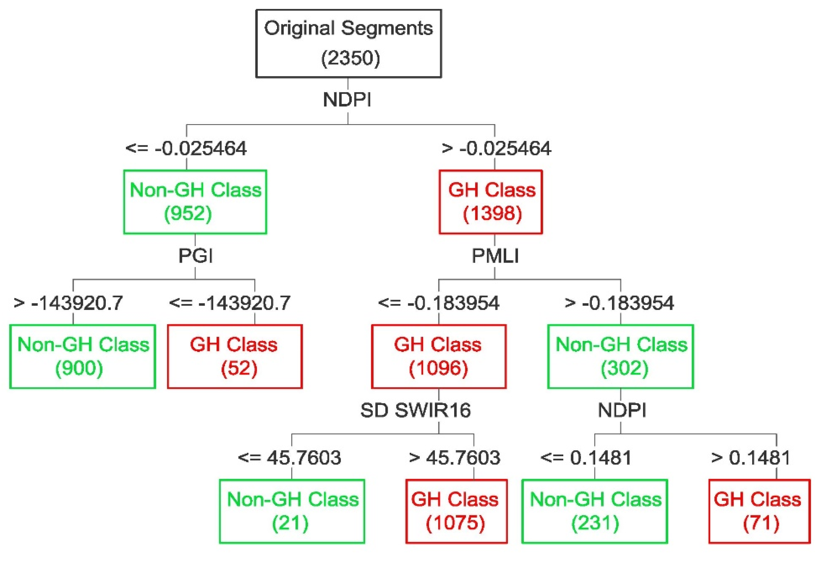
5.3. Importance of Features and Decision Tree Models
5.4. Pixel-Based Accuracy Assessment
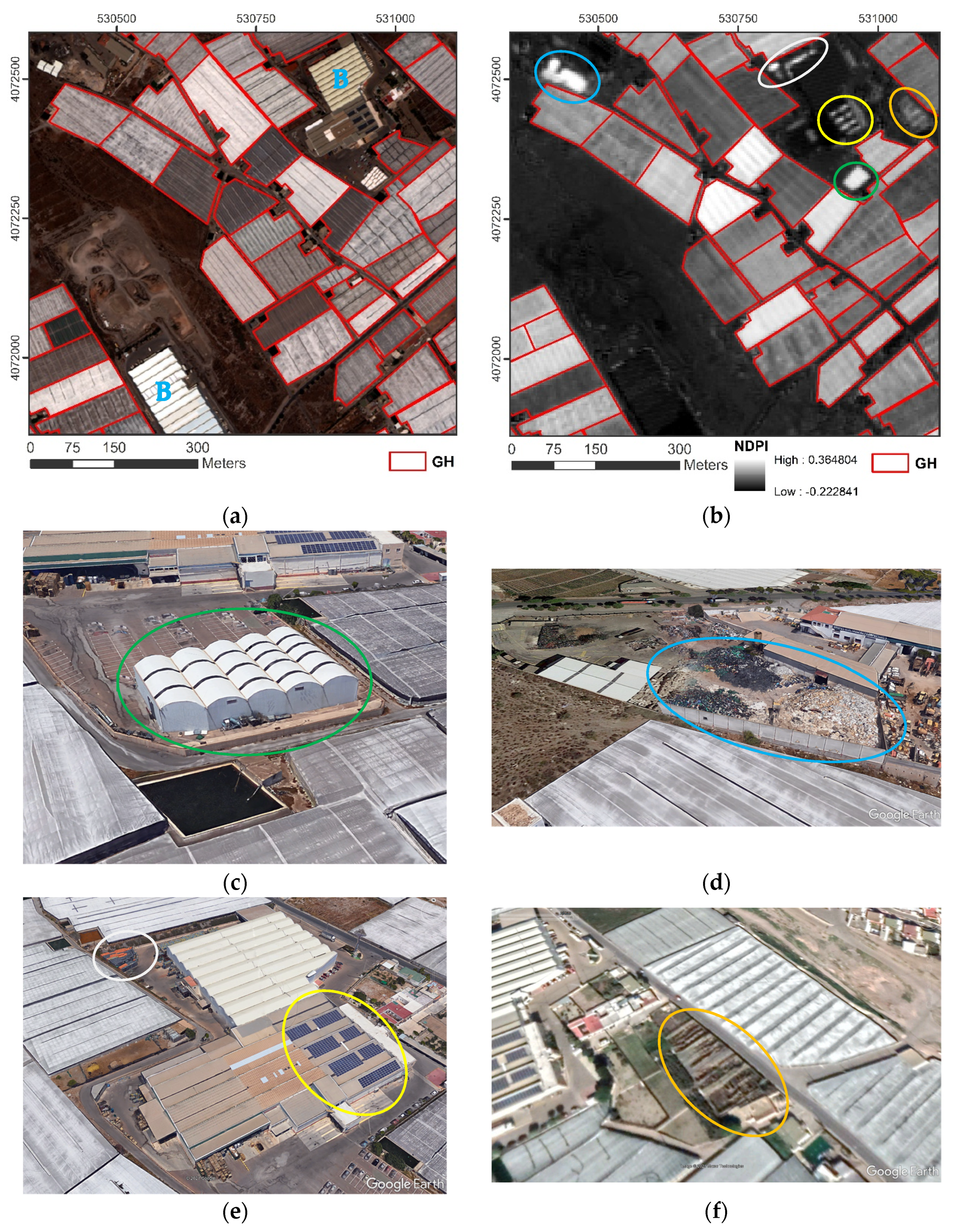
6. Discussion
7. Conclusions
Author Contributions
Funding
Acknowledgments
Conflicts of Interest
References
- Scarascia-Mugnozza, G.; Sica, C.; Russo, G. Plastic materials in European agriculture: Actual use and perspectives. J. Agric. Eng. 2012, 42, 15–28. [Google Scholar] [CrossRef]
- Atzberger, C. Advances in Remote Sensing of Agriculture: Context Description, Existing Operational Monitoring Systems and Major Information Needs. Remote Sens. 2013, 5, 949–981. [Google Scholar] [CrossRef]
- Aguilar, M.A.; Vallario, A.; Aguilar, F.J.; Lorca, A.G.; Parente, C. Object-Based Greenhouse Horticultural Crop Identification from Multi-Temporal Satellite Imagery: A Case Study in Almeria, Spain. Remote Sens. 2015, 7, 7378–7401. [Google Scholar] [CrossRef]
- Lanorte, A.; De Santis, F.; Nolè, G.; Blanco, I.; Loisi, R.V.; Schettini, E.; Vox, G. Agricultural plastic waste spatial estimation by Landsat 8 satellite images. Comput. Electron. Agric. 2017, 141, 35–45. [Google Scholar] [CrossRef]
- Jiménez-Lao, R.; Aguilar, F.; Nemmaoui, A.; Aguilar, M. Remote Sensing of Agricultural Greenhouses and Plastic-Mulched Farmland: An Analysis of Worldwide Research. Remote Sens. 2020, 12, 2649. [Google Scholar] [CrossRef]
- WorldView-3 Datasheet (DigitalGlobe, 2014). Available online: http://satimagingcorp.s3.amazonaws.com/site/pdf/WorldView3-DS-WV3-Web.pdf (accessed on 12 April 2021).
- Acuña-Ruz, T.; Uribe, D.; Taylor, R.; Amézquita, L.; Guzmán, M.C.; Merrill, J.; Martínez, P.; Voisin, L.; Mattar, B.C. Anthropogenic marine debris over beaches: Spectral characterization for remote sensing applications. Remote Sens. Environ. 2018, 217, 309–322. [Google Scholar] [CrossRef]
- Biermann, L.; Clewley, D.; Martinez-Vicente, V.; Topouzelis, K. Finding Plastic Patches in Coastal Waters using Optical Satellite Data. Sci. Rep. 2020, 10, 1–10. [Google Scholar] [CrossRef]
- Themistocleous, K.; Papoutsa, C.; Michaelides, S.; Hadjimitsis, D. Investigating Detection of Floating Plastic Litter from Space Using Sentinel-2 Imagery. Remote Sens. 2020, 12, 2648. [Google Scholar] [CrossRef]
- Novelli, A.; Aguilar, M.A.; Nemmaoui, A.; Aguilar, F.J.; Tarantino, E. Performance evaluation of object based greenhouse detection from Sentinel-2 MSI and Landsat 8 OLI data: A case study from Almería (Spain). Int. J. Appl. Earth Obs. Geoinf. 2016, 52, 403–411. [Google Scholar] [CrossRef]
- Yang, D.; Chen, J.; Zhou, Y.; Chen, X.; Chen, X.; Cao, X. Mapping plastic greenhouse with medium spatial resolution satellite data: Development of a new spectral index. ISPRS J. Photogramm. Remote Sens. 2017, 128, 47–60. [Google Scholar] [CrossRef]
- Lu, L.; Di, L.; Ye, Y. A Decision-Tree Classifier for Extracting Transparent Plastic-Mulched Landcover from Landsat-5 TM Images. IEEE J. Sel. Top. Appl. Earth Obs. Remote Sens. 2014, 7, 4548–4558. [Google Scholar] [CrossRef]
- Hasituya; Chen, Z.; Wang, L.; Wu, W.; Jiang, Z.; Li, H. Monitoring Plastic-Mulched Farmland by Landsat-8 OLI Imagery Using Spectral and Textural Features. Remote Sens. 2016, 8, 353. [Google Scholar] [CrossRef]
- Guo, X.; Li, P. Mapping plastic materials in an urban area: Development of the normalized difference plastic index using WorldView-3 superspectral data. ISPRS J. Photogramm. Remote Sens. 2020, 169, 214–226. [Google Scholar] [CrossRef]
- Asadzadeh, S.; de Souza Filho, C.R. Investigating the capability of WorldView-3 superspectral data for direct hydrocarbon detection. Remote Sens. Environ. 2016, 173, 162–173. [Google Scholar] [CrossRef]
- American Chemistry Council. 2019, Plastics 101. Available online: https://plastics.americanchemistry.com/Plastics-101/ (accessed on 22 April 2021).
- Levin, N.; Lugassi, R.; Ramon, U.; Braun, O.; Ben-Dor, E. Remote sensing as a tool for monitoring plasticulture in agricultural landscapes. Int. J. Remote Sens. 2007, 28, 183–202. [Google Scholar] [CrossRef]
- Garaba, S.P.; Dierssen, H.M. An airborne remote sensing case study of synthetic hydrocarbon detection using short wave infrared absorption features identified from marine-harvested macro- and microplastics. Remote Sens. Environ. 2018, 205, 224–235. [Google Scholar] [CrossRef]
- Berk, A.; Bernstein, L.; Anderson, G.; Acharya, P.; Robertson, D.; Chetwynd, J.; Adler-Golden, S. MODTRAN Cloud and Multiple Scattering Upgrades with Application to AVIRIS. Remote Sens. Environ. 1998, 65, 367–375. [Google Scholar] [CrossRef]
- Blaschke, T. Object based image analysis for remote sensing. ISPRS J. Photogramm. Remote Sens. 2010, 65, 2–16. [Google Scholar] [CrossRef]
- Aguilar, M.A.; Nemmaoui, A.; Novelli, A.; Aguilar, F.J.; Lorca, A.G. Object-Based Greenhouse Mapping Using Very High Resolution Satellite Data and Landsat 8 Time Series. Remote Sens. 2016, 8, 513. [Google Scholar] [CrossRef]
- Nemmaoui, A.; Aguilar, M.A.; Aguilar, F.J.; Novelli, A.; Lorca, A.G. Greenhouse Crop Identification from Multi-Temporal Multi-Sensor Satellite Imagery Using Object-Based Approach: A Case Study from Almería (Spain). Remote Sens. 2018, 10, 1751. [Google Scholar] [CrossRef]
- Novelli, A.; Aguilar, M.A.; Aguilar, F.J.; Nemmaoui, A.; Tarantino, E. AssesSeg—A Command Line Tool to Quantify Image Segmentation Quality: A Test Carried Out in Southern Spain from Satellite Imagery. Remote Sens. 2017, 9, 40. [Google Scholar] [CrossRef]
- Aguilar, M.A.; Novelli, A.; Nemamoui, A.; Aguilar, F.J.; García Lorca, A.; González-Yebra, Ó. Optimizing Multiresolution Segmentation for Extracting Plastic Greenhouses from WorldView-3 Imagery. In Intelligent Interactive Multimedia Systems and Services 2017. KES-IIMSS-18 2018. Smart Innovation, Systems and Technologies; De Pietro, G., Gallo, L., Howlett, R., Jain, L., Eds.; Springer: Cham, Switzerland, 2018; Volume 76. [Google Scholar] [CrossRef]
- Liu, Y.; Bian, L.; Meng, Y.; Wang, H.; Zhang, S.; Yang, Y.; Shao, X.; Wang, B. Discrepancy measures for selecting optimal combination of parameter values in object-based image analysis. ISPRS J. Photogramm. Remote Sens. 2012, 68, 144–156. [Google Scholar] [CrossRef]
- Trimble Germany GmbH. Trimble eCognition Developer for Windows Operating System, Reference Book; Trimble Germany GmbH: Munich, Germany, 2019. [Google Scholar]
- Rouse, J.W.; Haas, R.H.; Schell, J.A.; Deering, D.W. Monitoring vegetation systems in the great plains with ERTS. Proc. Third ERTS Symp. 1973, 1, 48–62. [Google Scholar]
- Breiman, L.; Friedman, J.H.; Olshen, R.A.; Stone, C.I. Classification and Regression Trees; Chapman & Hall/CRC Press: Boca Raton, FL, USA, 1984. [Google Scholar]
- Zambon, M.; Lawrence, R.; Bunn, A.; Powell, S. Effect of Alternative Splitting Rules on Image Processing Using Classification Tree Analysis. Photogramm. Eng. Remote Sens. 2006, 72, 25–30. [Google Scholar] [CrossRef]
- Vieira, M.A.; Formaggio, A.R.; Rennó, C.D.; Atzberger, C.; Aguiar, D.A.; Mello, M.P. Object Based Image Analysis and Data Mining applied to a remotely sensed Landsat time-series to map sugarcane over large areas. Remote Sens. Environ. 2012, 123, 553–562. [Google Scholar] [CrossRef]
- Congalton, R.G. A review of assessing the accuracy of classifications of remotely sensed data. Remote Sens. Environ. 1991, 37, 35–46. [Google Scholar] [CrossRef]
- Kotaridis, I.; Lazaridou, M. Remote sensing image segmentation advances: A meta-analysis. ISPRS J. Photogramm. Remote Sens. 2021, 173, 309–322. [Google Scholar] [CrossRef]
- González-Yebra, Ó.; Aguilar, M.A.; Nemmaoui, A.; Aguilar, F.J. Methodological proposal to assess plastic greenhouses land cover change from the combination of archival aerial orthoimages and Landsat data. Biosyst. Eng. 2018, 175, 36–51. [Google Scholar] [CrossRef]
- Ou, C.; Yang, J.; Du, Z.; Liu, Y.; Feng, Q.; Zhu, D. Long-Term Mapping of a Greenhouse in a Typical Protected Agricultural Region Using Landsat Imagery and the Google Earth Engine. Remote Sens. 2019, 12, 55. [Google Scholar] [CrossRef]
- Balcik, F.B.; Senel, G.; Goksel, C. Object-Based Classification of Greenhouses Using Sentinel-2 MSI and SPOT-7 Images: A Case Study from Anamur (Mersin), Turkey. IEEE J. Sel. Top. Appl. Earth Obs. Remote Sens. 2020, 13, 2769–2777. [Google Scholar] [CrossRef]
- Hasituya; Zhongxin, C.; Fei, L.; Yuncai, H. Mapping plastic-mulched farmland by coupling optical and synthetic aperture radar remote sensing. Int. J. Remote Sens. 2020, 41, 7757–7778. [Google Scholar] [CrossRef]
- Vangi, E.; D’Amico, G.; Francini, S.; Giannetti, F.; Lasserre, B.; Marchetti, M.; Chirici, G. The New Hyperspectral Satellite PRISMA: Imagery for Forest Types Discrimination. Sensors 2021, 21, 1182. [Google Scholar] [CrossRef]

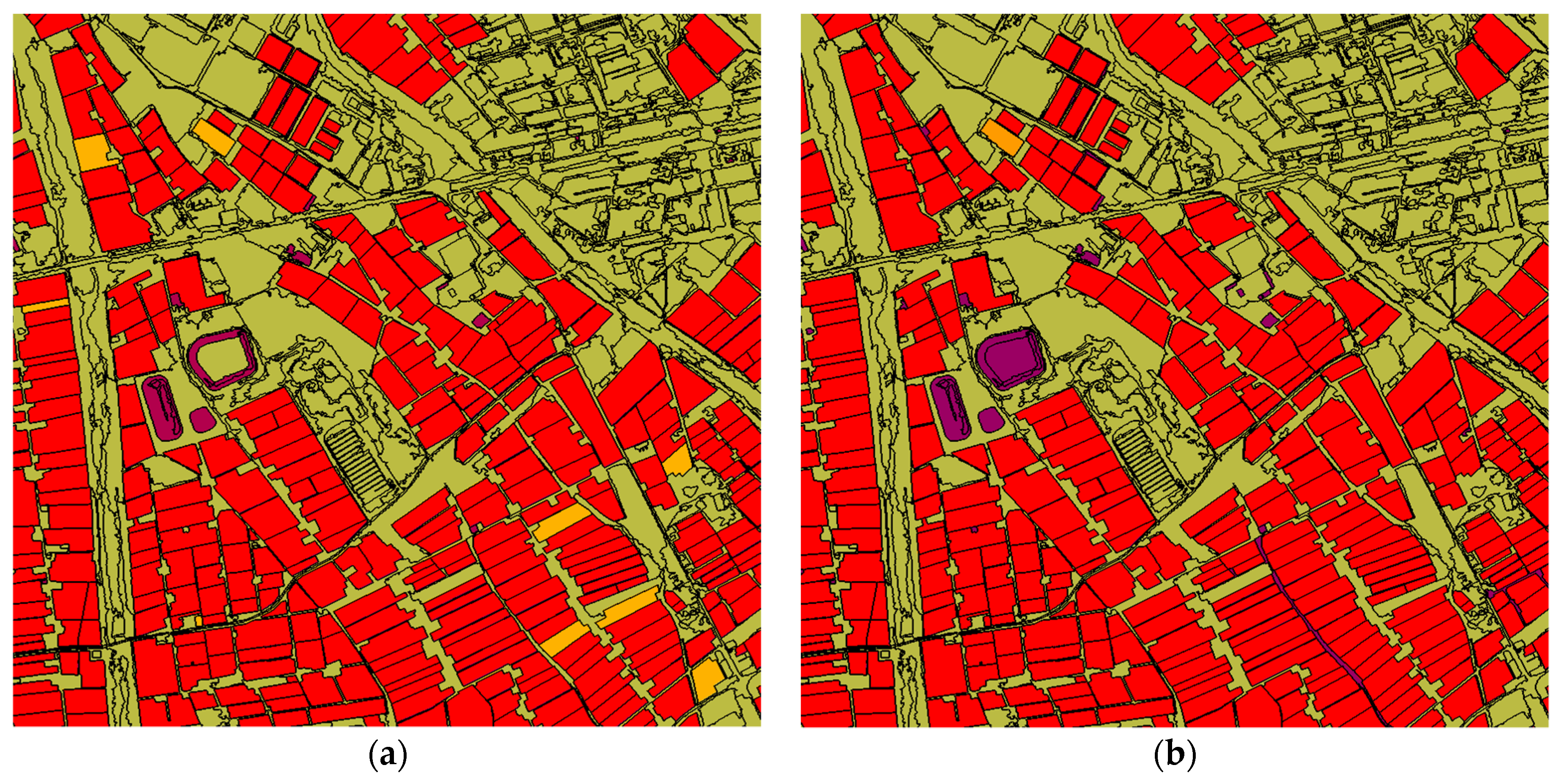
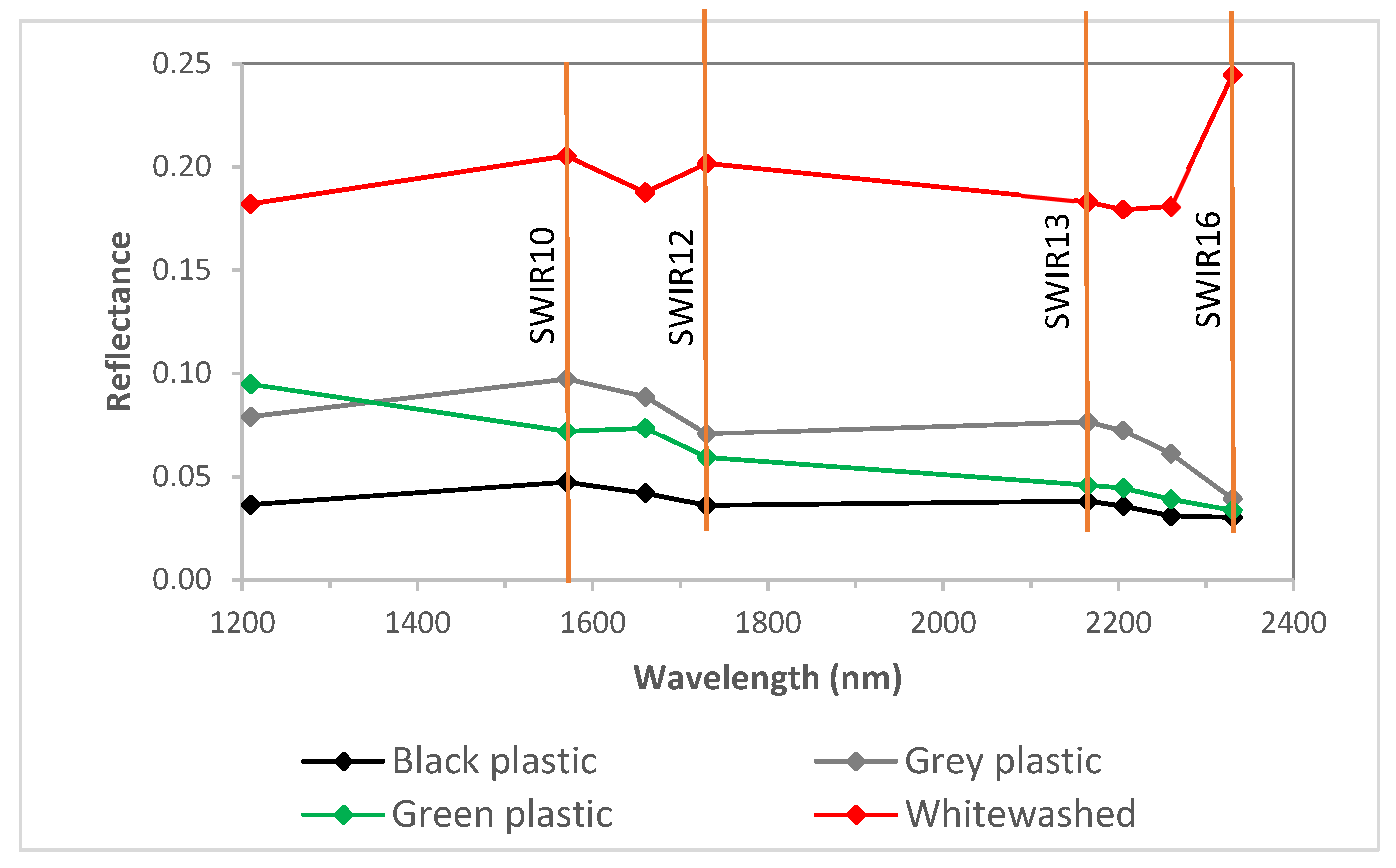
| Band | Band Name | Image | Wavelengths (nm) | Band | Band Name | Image | Wavelengths (nm) |
|---|---|---|---|---|---|---|---|
| PAN | PAN | 450–800 | |||||
| 1 | Coastal (C) | VNIR | 400–450 | 9 | SWIR9 | SWIR | 1195–1225 |
| 2 | Blue (B) | 450–510 | 10 | SWIR10 | 1550–1590 | ||
| 3 | Green (G) | 510–580 | 11 | SWIR11 | 1640–1680 | ||
| 4 | Yellow (Y) | 585–625 | 12 | SWIR12 | 1710–1750 | ||
| 5 | Red (R) | 630–690 | 13 | SWIR13 | 2145–2185 | ||
| 6 | Red Edge (RE) | 705–745 | 14 | SWIR14 | 2185–2225 | ||
| 7 | NIR1 | 770–895 | 15 | SWIR15 | 2235–2285 | ||
| 8 | NIR2 | 860–1040 | 16 | SWIR16 | 2295–2365 |
| Source | Name | Definitions | References |
|---|---|---|---|
| VNIR | Mean and standard deviation (SD) (16 features) | Mean and SD of each of 1 to 8 band | [26] |
| Brightness | Average value for all 8 VNIR bands | [26] | |
| NDVI (Normalized Difference Vegetation Index) | (NIR2 − R)/(NIR2 + R) | [27] | |
| PGI (Plastic Greenhouse Index) | 100 × (B × (NIR2 − R))/(1 − (B + G + NIR2)/3) | [11] | |
| PI (Plastic Index) | NIR2/(NIR2 + R) | [9] | |
| SWIR | Mean and standard deviation (SD) (16 features) | Mean and SD of each of 9 to 16 band | [26] |
| NDPI (Normalized Difference Plastic Index) | ((SWIR10 − SWIR12) + (SWIR13 − SWIR16))/(SWIR10 + SWIR12 + SWIR13 + SWIR16) | [14] | |
| PMLI (Plastic–Mulched Landcover Index) | (SWIR10 – R)/(SWIR10 + R) | [12] | |
| RBD (Relative-absorption Band Depth index) | (SWIR11 − SWIR13)/SWIR13) | [15] |
| Strategy | User/reference | GH | Non-GH | Sum |
|---|---|---|---|---|
| All Features | GH | 1147 | 28 | 1175 |
| Non-GH | 51 | 1124 | 1175 | |
| Sum | 1198 | 1152 | 2350 | |
| OA (%) = 96.64 | kappa = 0.933 | |||
| VNIR | GH | 1034 | 141 | 1175 |
| Non-GH | 103 | 1072 | 1175 | |
| Sum | 1137 | 1213 | 2350 | |
| OA (%) = 89.62 | kappa = 0.792 | |||
| SWIR | GH | 1138 | 37 | 1175 |
| Non-GH | 79 | 1096 | 1175 | |
| Sum | 1217 | 1133 | 2350 | |
| OA (%) = 95.06 | kappa = 0.901 | |||
| All Features | VNIR | SWIR | |||
|---|---|---|---|---|---|
| Feature | Importance | Feature | Importance | Feature | Importance |
| NDPI | 1.000 | Mean C | 1.000 | NDPI | 1.000 |
| PMLI | 0.968 | Mean B | 0.926 | PMLI | 0.956 |
| Mean C | 0.818 | PI | 0.862 | SD SWIR12 | 0.439 |
| PGI | 0.779 | NDVI | 0.862 | SD SWIR11 | 0.425 |
| Mean B | 0.759 | PGI | 0.781 | SD SWIR14 | 0.418 |
| Brightness | 0.711 | Mean G | 0.780 | SD SWIR10 | 0.417 |
| Mean G | 0.705 | Mean Y | 0.671 | SD SWIR13 | 0.413 |
| Mean RE | 0.660 | Brightness | 0.659 | SD SWIR15 | 0.411 |
| Mean Y | 0.647 | Mean R | 0.646 | SD SWIR16 | 0.403 |
| Mean R | 0.633 | SD R | 0.609 | Mean SWIR16 | 0.395 |
| Strategy | User/reference | GH | Non-GH | Sum |
|---|---|---|---|---|
| All Features | GH | 8,691,478 | 97,357 | 8,788,835 |
| Non-GH | 278,134 | 5,271,465 | 5,549,599 | |
| Sum | 8,969,612 | 5,368,822 | 14,338,434 | |
| OA (%) = 97.38 | kappa = 0.944 | |||
| GH UA (%) = 98.89 | GH PA (%) = 96.90 | |||
| VNIR | GH | 7,791,948 | 134,237 | 7,926,185 |
| Non-GH | 1,177,664 | 5,234,585 | 6,412,249 | |
| Sum | 8,969,612 | 5,368,822 | 14,338,434 | |
| OA (%) = 90.85 | kappa = 0.812 | |||
| GH UA (%) = 98.31 | GH PA (%) = 86.87 | |||
| SWIR | GH | 8,622,938 | 113,534 | 8,736,472 |
| Non-GH | 346,674 | 5,255,288 | 5,601,962 | |
| Sum | 8,969,612 | 5,368,822 | 14,338,434 | |
| OA (%) = 96.79 | kappa = 0.932 | |||
| GH UA (%) = 98.70 | GH PA (%) = 96.14 | |||
| Strategy | User/reference | GH | Non-GH | Sum |
|---|---|---|---|---|
| NDPI_B | GH | 8,905,137 | 211,147 | 9,116,284 |
| Non-GH | 64,475 | 5,157,675 | 5,222,150 | |
| Sum | 8,969,612 | 5,368,822 | 14,338,434 | |
| OA (%) = 98.08 | kappa = 0.959 | |||
| GH UA (%) = 97.68 | GH PA (%) = 99.28 | |||
Publisher’s Note: MDPI stays neutral with regard to jurisdictional claims in published maps and institutional affiliations. |
© 2021 by the authors. Licensee MDPI, Basel, Switzerland. This article is an open access article distributed under the terms and conditions of the Creative Commons Attribution (CC BY) license (https://creativecommons.org/licenses/by/4.0/).
Share and Cite
Aguilar, M.A.; Jiménez-Lao, R.; Aguilar, F.J. Evaluation of Object-Based Greenhouse Mapping Using WorldView-3 VNIR and SWIR Data: A Case Study from Almería (Spain). Remote Sens. 2021, 13, 2133. https://doi.org/10.3390/rs13112133
Aguilar MA, Jiménez-Lao R, Aguilar FJ. Evaluation of Object-Based Greenhouse Mapping Using WorldView-3 VNIR and SWIR Data: A Case Study from Almería (Spain). Remote Sensing. 2021; 13(11):2133. https://doi.org/10.3390/rs13112133
Chicago/Turabian StyleAguilar, Manuel A., Rafael Jiménez-Lao, and Fernando J. Aguilar. 2021. "Evaluation of Object-Based Greenhouse Mapping Using WorldView-3 VNIR and SWIR Data: A Case Study from Almería (Spain)" Remote Sensing 13, no. 11: 2133. https://doi.org/10.3390/rs13112133
APA StyleAguilar, M. A., Jiménez-Lao, R., & Aguilar, F. J. (2021). Evaluation of Object-Based Greenhouse Mapping Using WorldView-3 VNIR and SWIR Data: A Case Study from Almería (Spain). Remote Sensing, 13(11), 2133. https://doi.org/10.3390/rs13112133


