Abstract
Air–sea heat fluxes are essential climate variables, required for understanding air–sea interactions, local, regional and global climate, the hydrological cycle and atmospheric and oceanic circulation. In situ measurements of fluxes over the ocean are sparse and model reanalysis and satellite data can provide estimates at different scales. The accuracy of such estimates is therefore essential to obtain a reliable description of the occurring phenomena and changes. In this work, air–sea radiative fluxes derived from the SEVIRI sensor onboard the MSG satellite and from ERA5 reanalysis have been compared to direct high quality measurements performed over a complete annual cycle at the ENEA oceanographic observatory, near the island of Lampedusa in the Central Mediterranean Sea. Our analysis reveals that satellite derived products overestimate in situ direct observations of the downwelling short-wave (bias of 6.1 W/m2) and longwave (bias of 6.6 W/m2) irradiances. ERA5 reanalysis data show a negligible positive bias (+1.0 W/m2) for the shortwave irradiance and a large negative bias (−17 W/m2) for the longwave irradiance with respect to in situ observations. ERA5 meteorological variables, which are needed to calculate the air–sea heat flux using bulk formulae, have been compared with in situ measurements made at the oceanographic observatory. The two meteorological datasets show a very good agreement, with some underestimate of the wind speed by ERA5 for high wind conditions. We investigated the impact of different determinations of heat fluxes on the near surface sea temperature (1 m depth), as determined by calculations with a one-dimensional numerical model, the General Ocean Turbulence Model (GOTM). The sensitivity of the model to the different forcing was measured in terms of differences with respect to in situ temperature measurements made during the period under investigation. All simulations reproduced the true seasonal cycle and all high frequency variabilities. The best results on the overall seasonal cycle were obtained when using meteorological variables in the bulk formulae formulations used by the model itself. The derived overall annual net heat flux values were between +1.6 and 40.4 W/m2, depending on the used dataset. The large variability obtained with different datasets suggests that current determinations of the heat flux components and, in particular, of the longwave irradiance, need to be improved. The ENEA oceanographic observatory provides a complete, long-term, high resolution time series of high quality in situ observations. In the future, more similar sites worldwide will be needed for model and satellite validations and to improve the determination of the air–sea exchange and the understanding of related processes.
1. Introduction
The ocean interacts with the atmosphere by means of exchanges of momentum, heat, water, gases and particles at the air–sea interface, defining its energy and mass balance and consequently its role in the regional and global climate system at all spatial and temporal scales [1,2].
Air–sea heat fluxes (Figure 1) are essential drivers of the climate system, controlling interaction processes from sub-diurnal to multi-decadal time scales and from regional to global scales. The determination of the accuracy of the fluxes at the air–sea interface, either retrieved from satellites or modelled, is essential for a correct assessment of the total heat budget. In its turn, the assessment is fundamental for improving climate models and their forecast skills. Determining the components of the surface heat budget is also critical to a complete understanding of the water budget and the regional climate, especially in regions such as the Mediterranean Sea, a semi-enclosed basin surrounded by continental regions with complex orography and evident constraints in terms of mass and heat budget closure. In the specific case of the Mediterranean Sea, the “heat budget closure problem” described by several authors [2,3,4,5] states that that the long-term mean of the heat flux gained through the Gibraltar Strait by advection must be compensated by the net heat loss at the surface integrated over the whole basin. This heat compensation should ensure numerical closure of the basin’s water budget.
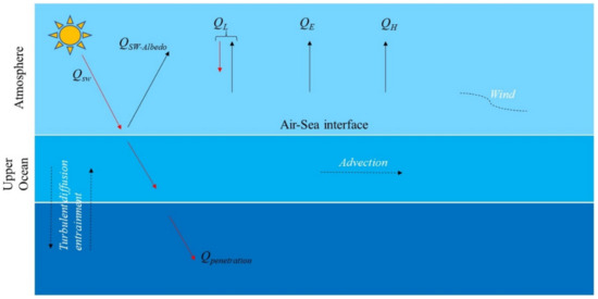
Figure 1.
Pictorial view of the air–sea heat exchange components.
Estimates of the mean Mediterranean heat exchange between ocean and atmosphere range from −11 to +22 W/m2, with an evident dominance of negative estimates, i.e., heat loss from the ocean to the atmosphere [5,6,7,8,9,10,11]. Some studies suggest that the Mediterranean heat budget is close to a neutral value, −1 W/m2 [12] or +1 W/m2 [13]. The non-negligible uncertainty on the estimation of heat flux components and the large variety of contrasting estimates of the basin-wide net air–sea heat fluxes in the Mediterranean Sea, prevent the achievement of an adequate solution for the problem of closing the Mediterranean heat balance. This open question highlights the need to assess and, if possible, minimize the uncertainties on the estimation of each component of the air–sea heat balance.
The net surface heat budget can be expressed as the sum of four distinct components:
where QS = QSW *(1 − α) is the net shortwave radiation flux, α is the ocean surface albedo, QSW is the downwelling shortwave radiation flux, QL is the net longwave radiation flux, QE is the latent heat flux and QH is the sensible heat flux.
Direct measurements of turbulent fluxes (i.e., latent and sensible heat fluxes) over the ocean are particularly rare. These measurements are only occasionally available at a very limited number of sites. The paucity of such information is caused by the difficulties of acquiring vertical wind components and high-frequency fluctuations in temperature and humidity in the often hostile marine environment onboard vessels and/or equipped fixed-platforms (e.g., mooring/buoys), while minimizing flow distortions due to the movement and shape of the platform housing the instruments [14,15]. In practice, the most common approach, even within numerical climate modeling, is to use empirical methods to estimate the various components of air–sea heat (or momentum) exchange by linking micro-scale turbulent transfer to more easily measurable macroscopic quantities, such as near-surface wind intensity, humidity or temperature. This approach requires a thorough assessment of the uncertainty on measurements of macroscopic environmental variables that enter in empirical formulas and, ultimately, of bulk formulae performances. In the last decades, various parameterizations of turbulent fluxes have been developed with varying levels of sophistication, ranging from the “inertial-dissipation method” [16,17], essentially an application of Kolmogorov theory for estimating turbulent fluxes, to “bulk aerodynamic methods” based on Monin–Obukhov similarity theory [18,19,20].
The turbulent components of the net heat flux, i.e., the sensible () and latent () heat fluxes as well as the wind stress () can be written in terms of “Reynolds Averages” [20]:
where w’, T’, q’ and u’ represent the turbulent fluctuations of the vertical component of the wind vector, temperature, mixing ratio and wind horizontal component, respectively and the variables with an asterisk can be considered as scaling parameters in terms of Monin–Obukhov similarity theory [20,21]. The brackets denote the ensemble average, which, in fact, are approximated by averages over time or space of finite data sets, by assuming process ergodicity.
The “bulk” version of Equations (2)–(4), where scalar fluxes and wind stress components are expressed in terms of macroscopic variables commonly measured in meteorological practice, is:
where Ch, Ce and Cd are the turbulent transfer coefficients for the sensible and latent heat fluxes and wind stress, respectively; is the air density; Le is the evaporation latent heat, is the mean horizontal wind value at a given height above the surface, z; Ts is the temperature at the air–sea interface; Ta is the air temperature at z; qa and qs are the specific humidity at z and the saturation humidity at the sea surface temperature Ts, possibly corrected for the effect of salinity, respectively. Finally, the difference represents the wind speed relative to the surface ocean current usl. Regarding the values to be used for the turbulent transfer coefficients Ch, Ce and Cd, there is a large body of literature that suggests how to estimate their values as a function of usually available meteorological variables [20,22,23].
Direct measurements of the radiative budget at the sea are not abundant, but still far more numerous than those of turbulent fluxes, also in relation to the relative lower complexity of execution. This has allowed the proliferation of various regression-based formulations for estimating coefficients of empirical formulas aimed at minimizing differences with direct measurements. Regarding the most popular empirical formulae for estimating the two components of the radiative budget, validation exercises in the Mediterranean Sea were described [24,25,26]. In many operational contexts and numerical models, the short-wave (insolation) budget is calculated based the formulas of Reed [27] and Simpson and Paulson [28]. These were adapted by Rosati and Miyakoda [29] as:
where Qs,Clear represents the shortwave radiation reaching the sea surface under clear sky conditions [26], C is the fraction of cloud cover, is the sun elevation at noon (in degree) and α is the surface albedo. This is the formulation used in most OGCMs (Ocean General Circulation Model) for calculating the shortwave budget at the air–sea interface. In the case of the net longwave radiation flux, several empirical formulations were developed [7,25,30,31,32,33,34,35,36]. All of these empirical formulas produce estimates of the longwave net flux as a function of sea surface temperature (SST), air temperature (Ta), water vapor pressure e (or humidity q) and cloud cover fraction C. The formula of Bignami et al. (1995) [25]:
This formula was specifically designed for the Mediterranean Sea and is currently used in ocean operational forecast systems and research studies for this basin [37,38,39,40].
Reliable heat flux data values at each grid point of the Mediterranean Sea are needed to determine its total heat budget. The combined use of numerical models or reanalysis data and satellite data is thus essential for these basin-wide estimates. Both have synoptic coverage but different temporal and spatial resolutions, e.g., the European Centre for Medium-Range Weather Forecasts (ECMWF) Reanalysis 5th Generation (ERA5; https://confluence.ecmwf.int/display/CKB/ERA5%3A+data+documentation (last accessed on 21 March 2019) data are globally distributed at hourly frequency and spatial resolution of 0.25 × 0.25 degrees, while Meteosat Second Generation (MSG) surface shortwave and longwave irradiance data are distributed on hourly basis but at 0.05 × 0.05 degrees resolution. In such a context, the comparison between heat flux components estimates and direct measurements is crucial to assess the goodness of heat flux existing datasets. This implies the validation of the meteorological parameters that contribute to heat flux estimates in empirical formulae and the comparison of direct measurements with empirical and modelled estimates. Given that errors in estimated fluxes are not great or small per se, but in relation to a targeted application, a reasonable choice is to evaluate their impact on some predicted environmental variable such as the near surface sea water temperature.
Evaluation of reanalysis products has already been done in several areas globally, mostly over land (e.g., [41]). Over ocean, studies are much rarer, which is particularly true for the radiative components of the energy budget, where ocean in situ measurements are scarce. In addition, ERA5 is a relatively recent reanalysis and then no many formal validation reports for several dataset over the ocean have been published. Among those existing, the accuracy of MERRA-2 and ERA-Interim SST, air temperature and humidity profiles was evaluated over the Atlantic Ocean [42]. Another work, comparing hourly solar irradiation data from MERRA-2 and ERA5 over PIRATA (Pilot Research Moored Array in the Tropical Atlantic) buoys in the Atlantic Ocean found biases between −10 and +23 W/m2 and between −44 and +23 W/m2 for ERA5 and MERRA-2, respectively. RMS varied within the range 113 to 138 W/m2 for ERA5 and within 128 and 163 W/m2 for MERRA-2. The correlation coefficient ranged between 0.48 and 0.86 for ERA5 and between 0.29 and 0.80 for MERRA-2. [43]. Some additional evaluation was performed in the NW Iceland Sea [44] where a meteorological buoy worked for 78 days, producing valuable data for ERA5 assessment. Variables assessed where air temperature, SST, humidity, wind speed, momentum and latent and sensible turbulent fluxes, in particular for wind speed and air temperature (the variables in common between our and their analysis), biases, RMSE and correlation coefficient were: 0.61 m/s, 1.64 m/s, 0.92 and 0.05 °C, 1.11 °C and 0.92, respectively. The differences between ERA-Interim and ERA5 surface winds fields relative to Advanced Scatterometer (ASCAT) ocean vector wind observations were analyzed [45]. ERA5 winds showed a 20 % improvement relative to ERA-Interim in terms of instantaneous RMSE to ASCAT observations.
In this work, we validate both ERA5 reanalysis and satellite radiative flux estimates against quality-controlled in situ measurements, acquired at the Lampedusa Oceanographic Observatory [46] over a complete annual cycle (4 June 2017, to 3 June 2018). Despite the obvious limitation of using a single geographical location, the Lampedusa observatory offers the possibility of having a coherent, complete and quality-controlled time series over an entire annual cycle, experiencing a wide variety of Mediterranean climate conditions (e.g., strong insolation with stable atmospheric summer conditions and lower insolation with perturbed atmospheric stability in winter). To assess the impact of those differences between available heat fluxes datasets on simulations of key oceanographic variables, both global and regional ocean general circulation models (OGCMs) can be used, though with very high computational costs. Here, we use a sophisticated one-dimensional turbulence model, namely the GOTM (General Ocean Turbulence Model; www.gotm.net, accessed on 18 May 2021). This is a simplified but still physically meaningful model which contains all the components of air–sea heat exchange although lacking transport and thus horizontal advection. Thanks to its relatively low computational cost, GOTM permits to test a large variety of flux forcing at very high vertical resolution. However, the model is used as a diagnostic tool to identify the effect of changing heat budget components and is not intended to describe the medium and long-term evolution of the system.
The paper is structured as follows. Section 2 describes the data used in this analysis: ERA5 reanalysis, satellite data acquired by SEVIRI (www.eumetsat.int/seviri, accessed on 18 May 2021) and in situ observations at the Lampedusa Observatory. Some basic information on the GOTM software is also included. Section 3 shows direct evaluation of relevant ERA5 model and satellite SEVIRI products against the Lampedusa observations. Section 4 presents the impact of the different datasets on SST predictions by taking advantage of the year-long Lampedusa time series. The work concludes with some remarks based on these findings.
2. Data and Methods
2.1. In Situ Measurements
The measurements used in this study were carried out at the Lampedusa Oceanographic Observatory (OO), which is located in the open sea and in an strategic area representing indeed the boundary between the western and eastern part of the Mediterranean Sea. The buoy is located at 35.49°N, 12.47°E, about 3.3 nautical miles South West of the island of Lampedusa (Figure 2). The bottom depth at the buoy site is 74 m. The island belongs to the North-African continental shelf, with the Tunisian coast more than 100 km west of the buoy.
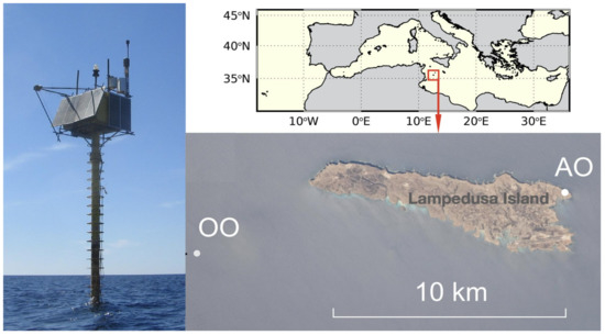
Figure 2.
The Oceanographic Observatory (OO, left panel) and its position near Lampedusa Island. AO indicates the position of the Atmospheric observatory. The Lampedusa island picture was taken from the International Space Station (picture ISS 024-E-10246; see acknowledgments).
The buoy was installed in 2015. The Oceanographic Observatory complements the Atmospheric Observatory (AO, 35.52°N, 12.63°E), built on the island of Lampedusa in 1997 and dedicated to climate studies (http://www.lampedusa.enea.it) (last accessed on 18 May 2021). The distance between the two observatories is about 15 km. A wide set of parameters related to climate are monitored at AO (e.g., meteorology, greenhouse gases, aerosols, radiation, clouds, etc.). However, this paper presents results only based on in situ data measured at OO.
The OO is primarily dedicated to investigating air–sea interactions. The buoy is of an elastic beacon type, designed to minimize structure oscillations and rotation. Nominally, the rotation of the buoy is <5° for sea state <4. Oscillations are also small: they are within ±1.7° along the West–East axis and within ±1.8° along the North-South axis for 90% of the time in January. The buoy is connected to an anchor, placed on the bottom. A vertical pylon about 8 m long emerges from water; a turret, which hosts the atmospheric sensors, is placed about 6.5 m above sea level. A more detailed description of the buoy characteristics is provided [46].
Measurements used in this analysis include various atmospheric and two submerged sensors. The list of instruments is reported in Table 1, together with the measured parameters, the position on the buoy and the period of operation on the buoy. Some sensors, like the radiometers and the ocean pressure/temperature recorders, are routinely replaced with freshly calibrated ones about once per year. The periods listed in Table 1 are relative to the measurements used in this analysis.

Table 1.
List of sensors, operational dates, parameters measured and positions at the OO. m.a.s.l. stands for meters above sea level.
All instruments were calibrated previously to deployment; the CMP21 solar radiometer was calibrated against instruments referred to the World Meteorological Organization World Radiation Reference scale, while the CGR4 infrared radiometer was referred to the World Infrared Standard Group, WISG (WMO, 2014) before and after deployment. More details on the radiometers’ calibration procedure can be found in di Sarra et al. [46]. The SBE39 recorders were calibrated by the manufacturer before deployment and at the Italian OGS (Istituto nazionale di Oceanografia e di Geofisica Sperimentale) after deployment; no change in the calibration coefficients was found. Calibration dates for all instruments are reported in Table 2.
Table 2.
List of instruments and calibrations at the OO.
The nominal accuracy of atmospheric temperature and humidity measurements is about 0.15 °C and 1–2%, respectively. The accuracy on atmospheric pressure measurement is ±0.2 hPa, while that on the wind measurement is ±2% on wind speed and ±3° on the direction. The nominal accuracy of the water temperature is ±0.002 °C and is ±0.002 dbar for water pressure [46].
Solar irradiance measurements are corrected for the thermal effect using the signal of the infrared sensor as recommended [46,47]. No correction for the instrument cosine response is implemented, due to the good instrumental response. The overall estimated uncertainty on the solar irradiance measurement is 1.7%, while it is ±5 W/m2 on the infrared irradiance. Buoy attitude and deposition of aerosol and humidity on the radiometers’ domes may affect both shortwave and longwave irradiance measurements. These effects were discussed [46], based on the comparison between simultaneous measurements made in 2016 at AO and OO. The root mean squared difference between the two sets of hourly average measurements is about 19 W/m2 for cloud-free daytime solar radiation and 8.6 W/m2 for nighttime infrared radiation and all sky conditions. The mean bias between daily average observations at OO and AO was −2.2 W/m2 for shortwave irradiance and was +6.2 W/m2 for longwave irradiance. These differences were found consistent with altitude and albedo differences between OO and AO, suggesting that highly accurate radiation observations are obtained at OO.
2.2. ERA5 Reanalysis
The reanalysis data used in this work come from the ERA5 dataset (1950–present). ERA5 is produced using 4D-Var data assimilation in CY41R2 of ECMWF’s Integrated Forecast System (IFS), with 137 hybrid sigma/pressure (model) levels in the vertical, with the top level at 0.01 hPa (IFS Documentation CY41R2-Part IV: Physical Processes). ERA5 also includes “surface or single level” data, containing 2D parameters such as precipitation, 2 m temperature, top of atmosphere radiation and vertical integrals over the entire atmosphere. The surface data are those used in this work. We downloaded hourly data from June 2017 to June 2018 relative to the closest grid point to the Lampedusa mooring from the Copernicus Climate Change Service (C3S) Climate Data Store (CDS) (https://cds.climate.copernicus.eu/#!/home) (last accessed on 2 June 2021). The parameters were selected on the basis of the corresponding mooring measurements considering also the list of variables that are typically used in empirical formulae, namely:
- Sea surface temperature;
- Air temperature near the surface (2 m from the surface);
- Dew point temperature (2 m from the surface);
- Cloud cover (fraction);
- Wind intensity (10 m from the surface, zonal and meridional components);
- Atmospheric pressure at the surface;
- Longwave Irradiance (LW);
- Shortwave Irradiance (SW).
2.3. Geostationary Satellite Irradiance Data
Satellite irradiance data is derived from hourly Spinning Enhanced Visible and Infrared Imager (SEVIRI) visible and thermal infrared measurements, onboard MSG. The products related to irradiance, i.e., Surface Solar Irradiance (SSI) and Downward Longwave Irradiance (DLI), are produced operationally and continuously by the EUMETSAT Ocean and Sea Ice Satellite Application Facility (OSI SAF). The algorithm used by OSI SAF to derive the instantaneous value of SSI is a physical parameterization applied separately to each pixel and is developed in a sequence of steps including calibration of counts in bi-directional reflectance, conversion from the narrow band of the satellite to the broader band of the solar spectrum, conversion of bi-directional reflectance to planetary albedo, parameterization for clear skies [48] and finally a parameterization of the effect of cloud cover [49].
The algorithm used by OSI SAF to derive the all-sky condition longwave irradiance is an empirical parameterization that uses the outputs of the ECMWF NWP model and corrects it with the cloudiness information obtained from the satellite. The estimation of this irradiance should be considered instantaneous since the cloud information, derived from the NWP SAF classification is instantaneous. These steps are described in some detail in OSI SAF’s Product User Manual (PUM) for both shortwave and longwave irradiances.
2.4. GOTM
The General Ocean Turbulence Model (GOTM; [50,51], see updated version on gotm.net; here, the MS Windows version 4.1 is used) is a one-dimensional water column model for studying hydrodynamic and biogeochemical processes in marine and limnic waters. GOTM includes a library of state-of-the-art turbulence closure models for the parameterization of vertical turbulent fluxes of momentum and heat. GOTM has been shown to be a useful tool for the study of evolution of thermal stratification [52], but other effects such as surface boundary layer dynamics, entrainment into bottom gravity currents, mixing in sloping bottom boundary layers and sediment dynamics can also be investigated. GOTM provides a useful platform to compare across many Ocean Surface Boundary Layer (OSBL) parameterizations. The successful modelling of turbulence within GOTM has led to the use of this module in ocean general circulation models such as the General Estuarine Transport Model (GETM), the Regional Ocean Modelling System (ROMS), the Nucleus for European Modelling of the Ocean (NEMO), the Semi-implicit Cross-scale Hydroscience Integrated System Model (SCHISM), the Finite Volume Community OceanModel (FVCOM) and the Proudman Oceanographic Laboratory Coastal Ocean Modelling System (POLCOMS).
3. Results and Discussion
3.1. Assessment of ERA5 Products
In situ data, measured at high temporal frequency, was averaged to the equivalent ERA 5 hourly resolution. Regarding spatial match, we selected the closest single grid point corresponding to the buoy position. A direct comparison between ERA5 hourly estimates of the main meteorological variables needed to calculate the heat fluxes and the corresponding measurements on the buoy is shown in Figure 3. There is an encouraging agreement between the ERA5 estimates and the in situ measurements, which gives confidence for subsequent estimates of the various heat flux components. Quantitatively, in terms of standard statistical metrics (mean bias, MB; root mean square error, RMSE; linear correlation coefficient, R; and slope of the linear fit between the two datasets), the distance between the ERA5 estimates and the in situ measurements is reported in Figure 3. Broadly, the differences between the in situ measurements and the reanalysis estimates are quite small and apparently non-dependent on the variable value. An exception can be found in the case of the wind intensity, that, as the intensity increases, shows an increasing underestimation by the reanalysis with respect to in situ data. This is underlined by the value of the slope of the regression line (Figure 3). Similar dependence of the bias on wind intensity was observed in the Gulf of Lion, Ligurian Sea and Aegean Sea comparing Quickscat data with blended wind data from ERA40, ECMWF analysis and NCEP (National Centers for Environmental Prediction) estimations [53]. On the other hand, an opposite effect was observed in the Iceland Sea where a 78 day time series was analyzed with and overestimation of the ERA5 wind intensity for high wind regimes [44], Figure 3c.
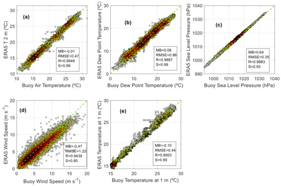
Figure 3.
Comparison between key meteorological variables contributing to air–sea heat flux estimates from ERA5 and from in situ observations. Air temperature (a), dew point temperature (b), atmospheric pressure at sea level (c), wind intensity (d), sea surface temperature (e). The (hourly) SST was inferred from the “skin” SST by adding the mean value of the difference with the “subskin” (0.17 °C) to make it more comparable with the sensor measurement at 1 m depth. Dot color indicates data density, increasing from white to black. Data refer to the period 3 June 2017–3 June 2018. Boxes within each plot include statistics of differences between ERA5 estimates and in situ measurements. Negative bias values indicate underestimates of the reanalysis.
The instruments mounted on board the Lampedusa buoy give the opportunity to verify the ERA5 estimates of shortwave and longwave downwelling irradiance. The scatterplots between the two datasets are shown in Figure 4. The shortwave irradiance shows a general good agreement, though with some underestimation of the ERA5 throughout the full range of values. The highly spread data points at the upper-left side of the panel are most likely produced under scattered clouds and denote the difficulty of ERA5 at pixel scale to correctly estimate rapidly varying cloud cover fraction over a given site at hourly scale. Differences of longwave irradiances seem to be more significant, but in line with the results of the shortwave irradiance comparison. Our results show much lower RMSE and much higher correlation with respect to another ERA5 assessment against PIRATA buoys in the tropical Atlantic Ocean [43], while our bias falls in their range of variability.
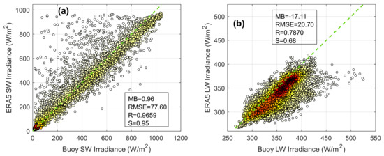
Figure 4.
Comparison between hourly shortwave (a) and longwave (b) irradiance estimated by ERA5 and corresponding values measured on the buoy. Dot color indicates data density, increasing from white to black. Data refer to the period 4 June 2017–3 June 2018. Units are W/m2. Boxes within each plot include statistics of differences between ERA5 estimates and in situ measurements of shortwave and longwave irradiance.
3.2. Assessment of Satellite Data
Hourly-averaged buoy data was matched to SEVIRI hourly data, extracted at the closest single pixel corresponding to the buoy position. The standard statistical indices of the comparison between satellite and buoy measurements are comparable with those reported for ERA5 (Figure 3 and Figure 5). The satellite shortwave irradiance shows a higher bias with respect to in situ data than ERA5, with a somewhat lower RMSE, while correlation and slope values are fully comparable with those obtained for ERA5. In the case of the longwave irradiance, the bias between satellite and in situ data is smaller in absolute value than that between ERA5 and in situ data and opposite in sign, indicating an overestimation of satellite-derived data, while RMSE and correlation values are similar to those found for ERA5. The slope is closer to the unit value than for ERA5.
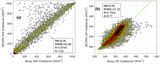
Figure 5.
Comparison between hourly shortwave (a) and longwave (b) irradiances estimated by SEVIRI and the corresponding values measured on the buoy. Dot color indicates data density, increasing from white to black. Data refer to the period June 2017–3 June 2018. Units are W/m2. Boxes within each plot include statistics of differences between satellite estimates and in situ measurements of shortwave and longwave irradiances.
3.3. Impact of Flux Differences on Numerical Simulations: A Case Study
Once the differences between estimates of relevant meteorological parameters and radiative fluxes have been determined, their consequent impact on GOTM model predictions is evaluated. The successive steps are to: (1) understand how relevant are these differences with respect to the subsequent applications; (2) understand the extent to which the available datasets are interchangeable and (3) establish user recommendations, based on the former findings.
The ideal setup would be to perform sensitivity experiments using general circulation models at global and regional scale either in forecast or in re-analysis mode, forced by the different available meteorological and flux data. Unfortunately, the computational cost of such an approach would be excessive and the implementation time would be well beyond the scope of this work. As an alternative, we carried out the sensitivity tests using a simplified but still physically meaningful model which contains all the components of air–sea heat exchange though lacks transport and thus horizontal advection. Here, we used the GOTM one-dimensional water column model for studying the variability of heat exchange processes under a variety of atmospheric forcing. GOTM solves the heat transport equation for temperature, incorporating the forcing and boundary conditions for each time step.
We forced GOTM with different heat components datasets such as those: (i) measured at the Lampedusa observatory; (ii) provided by ERA5 or (iii) estimated from satellite data. The GOTM simulation was started on 4 June 2017. Initial conditions were set as the average temperature and salinity vertical profiles, acquired very close to the buoy during an oceanographic cruise on 3 and 4 June 2017 (Figure 6). The vertical dimension was discretized into 140 vertical layers, with increased resolution towards the surface. At 1 m depth, the resolution was ~4 cm. The simulations were continued for 365 days until 3 June 2018, using a 60 s time step and storing the outputs hourly. The water temperature time series measured by a SBE39Plus sensor, T1m, was used as reference for the comparison for all the numerical simulations. Its average depth was 1 m, though subject to small instantaneous variations. The real sensor depth was determined from the measured pressure value; and the temperature modeled at the same depth was used in the comparison.

Figure 6.
In situ CTD casts made from 3 June 2017 at 14:00 UTC to 4 June 2017 at 07:56:00 UTC close to the Oceanographic Observatory. Dots represent individual CTD casts. The black lines represent the average profiles for temperature (a) and salinity (b) used as initial condition for the simulation.
Table 3 describes the general model configuration, including features such as turbulence modelling, light extinction parameterization and boundary conditions. The sum of net longwave irradiance, latent and sensible heat fluxes is used as a boundary condition in the model, while the solar radiation is treated as an internal heat source varying with depth as prescribed by Jerlov [54] (the so-called Jerlov-I attenuation model). Surface heat and momentum fluxes can be “prescribed”, intended as forcing GOTM with flux data directly, or indirectly set by means of meteorological data, which is used by GOTM to compute the fluxes using bulk formulas while running.
Table 3.
Options for the different GOTM parameters.
Table 4 describes all simulations (“experiments”) performed. All of them differed only in the air–sea heat fluxes. The first two experiments evaluated the impact of forcing GOTM with meteorological data coming from different sources. Near surface air and dew point temperature (2 m above the surface), cloud cover (fraction), wind intensity (10 m above the surface, zonal and meridional components) and surface atmospheric pressure were given to GOTM, either measured in situ at the buoy (experiment 1) or from ERA5 (experiment 2). However, because cloud cover fraction measurements were not available at the buoy site, both experiments were run using the ERA5 cloud cover fraction, implying that the net shortwave irradiance was the same for both.
Table 4.
Numerical summary of all experiments. For each forcing, it is given: the net ocean heat loss (latent + sensible + longwave), the heat gain due to shortwave and their sum. In addition, MB, RMSE and R are given, expressing the mean difference, root means square error and correlation coefficient of the simulated temperature respect to the temperature reference.
The water temperature at 1 m of depth (T1m) is shown in Figure 7a together with the measured value and Figure 7d shows the differences of the simulations to the latter. Table 4 reports the values of annual mean bias (MB), root mean square error (RMSE) and correlation coefficient (R) between the simulated and measured temperatures at 1 m depth. Both experiments 1 and 2 reproduced the annual cycle very well. Experiment 1 underestimated T1m by 0.08 °C (annual average), while experiment 2 overestimated T1m by 0.13 °C. The RMSE are 0.42 and 0.40 °C, respectively. This good agreement between both model simulations and measured data is somewhat surprising since the simulations were not aimed at reproducing the observations throughout a whole year, due to the lack of horizontal advection. What we can say based on the results obtained is that the differences between the buoy and the ERA5 meteorological variables are sufficiently small to produce very similar air sea heat and momentum exchanges that, in turn, produce a nearly identical water temperature evolution.
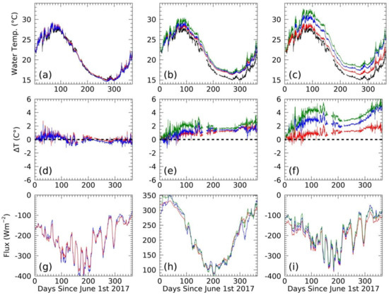
Figure 7.
Comparison between in situ measurements of water temperature at 1 m depth (black curves in (a–c)) and GOTM simulated water temperatures at the same depth obtained as follows: (a) Simulations using air–sea heat and momentum fluxes computed by the model at each time step, using bulk formulae with ERA5 meteorological parameters (experiment 1, red line) or bulk formulae with in situ meteorological parameters (experiment 2, blue line). (b) Simulations imposing air–sea heat and momentum fluxes obtained by ERA5 (experiment 3, red line), by ERA5 except for the shortwave irradiance, which is from in situ measurements (experiment 4, blue line) and by ERA5 except for the shortwave irradiance, which is estimated by SEVIRI (experiment 5, green line). (c) Simulations imposing air–sea heat and momentum fluxes obtained by ERA5 (experiment 3, red line), by ERA5 except for the longwave irradiance, which is form in situ observations at the buoy (experiment 6, blue line), by ERA5 except for the longwave irradiance, which is estimated by SEVIRI (experiment 7, green line). The differences between measured and simulated temperatures at 1 m depth are reported in panels d, e, f, for: (d) Experiment 1 (red) and experiment 2 (blue). (e) Experiment 3 (red), experiment 4 (blue) and experiment 5 (green). (f) Experiment 3 (red), experiment 6 (blue) and experiment 7 (green). (g) Ocean heat flux loss (latent + sensible + net longwave) computed by the model for experiment 1 (red) and experiment 2 (blue). (h) Shortwave component of the heat fluxes from in situ measurements (blue), ERA5 (red) and SEVIRI (green). (i) Ocean heat flux loss (latent+sensible+net longwave) for experiment 3 (red), experiment 6 (blue) and experiment 7 (green) A 10 days moving average filter has been applied to curves in panels (g–i) to enhance readability.
No conclusions must be extracted on the accuracy of single heat flux components because the overall effect is driven by the sum of the different contributions. The sum of the net longwave and turbulent fluxes is equal to the ocean total heat loss and its time series (10-day moving averages are displayed to improve readability) obtained from the experiments 1 and 2 is shown in Figure 7g. The corresponding values of the annual mean heat loss from the ocean to the atmosphere are reported in Table 4, amounting to 215.8 and 215.2 W/m2 for experiment 1 and experiment 2, respectively. This heat loss is balanced by 217.4 W/m2 of shortwave radiation that is transferred from the atmosphere to the ocean (as estimated by using Rosati and Miyakoda [29] and Payne [55]), giving a net positive ocean gains heat of 1.6 and 2.2 W/m2 for experiment 1 and 2, respectively.
Next simulations were performed with prescribed fluxes. A preliminary test, providing to GOTM the heat and momentum fluxes calculated applying the same bulk formulas and the same data used in experiments 1 and 2 (not shown), returned the same results of the “calculated by the model” version, giving us confidence that differences obtained by providing different heat fluxes can entirely be attributed to the selected dataset and not to differences of how bulk formulas are treated by the model or by ourselves.
A series of “prescribed fluxes” experiments was performed next, to evaluate the impact of varying the net shortwave radiation. Starting from the general setup in Table 3, ERA5 fluxes were given as inputs, except the shortwave radiation, which was either that from ERA5 (experiment 3; annual average of 216.6 W/m2), in situ buoy measurements (experiment 4, 215.7 W/m2) and SEVIRI (experiment 5, 221.7 W/m2). The corresponding simulated temperatures are shown in Figure 7b, the differences to the measured value in Figure 7e and the daily-averaged shortwave radiation is shown in Figure 7h. Annual values of heat loss are reported in Table 4. The use of these three different fluxes produced mean overestimations of T1m by 1.07 °C, 1.17 °C and 1.80 °C. The RMSE range between 0.55 °C and 0.61 °C. As evident from Figure 7, these biases are not constant over time. Indeed, if we focus on the first month of simulations, when the role of horizontal advection is expected to have produced a limited impact, the use of the measured shortwave irradiance produced a smaller bias with respect to T1m, of only −0.08 °C, while using ERA5 or SEVIRI the bias reached 0.21 °C and 0.53 °C, respectively. After the first month the bias tends to increase up to slightly more than 1 °C for experiment 3 and 4 and up to 1.8 °C for experiment 5.
Additional “prescribed fluxes” experiments were performed taking experiment 3 as reference, but this time, the longwave irradiance (LW) was varied. Compared to the −182.6 W/m2 of annual ocean heat loss in experiment 3, when LW came from in situ buoy LW measurements (experiment 6), the heat loss amounted to −182.6 W/m2 and when LW came from SEVIRI estimates (experiment 7) it resulted in heat loss of −176.2 W/m2 (Table 4). Contrarily to what happened in the experiments in which the SW irradiance was varied, here the simulated water temperatures diverged from T1m and from the ERA5 values nearly immediately after the start of the run, reaching biases of almost 1 °C after only a couple of weeks.
Looking at all experiments, it is interesting to note that in all cases the annual mean net heat budget was positive (the ocean gains heat). Its value varied between +1.6 W/m2 (experiment 2) and +40.4 W/m2 (experiment 7). Using different radiation datasets produced the largest changes in the net heat fluxes, while the use of ERA5 or measured meteorological parameters had a limited impact on the results, due to the high accuracy of ERA5 meteorology. Thus, reducing uncertainties on the radiative terms is essential for reducing uncertainties on the overall heat budget. In particular, the relative large biases in the reanalysis and satellite datasets for the longwave irradiance with respect to the in situ observations had a large impact, of the order of 22 W/m2, on the overall heat budget determinations.
4. Conclusions and Final Remarks
In this work, time series of meteorological data and radiative fluxes obtained from a marine observatory located in the central Mediterranean Sea have been used to locally validate reanalysis and satellite air–sea heat flux estimates. The comparison of simulated (ERA5) and measured meteorological variables is very encouraging for their use in many oceanographic and, more generally, environmental applications (see Table 1 and Figure 3). Biases are very small and generally not correlated with the measurements. The sole exception can be found in the ERA5 wind speed that exhibits a clear tendency of the bias to linearly increase with increasing wind intensity (Figure 8a).
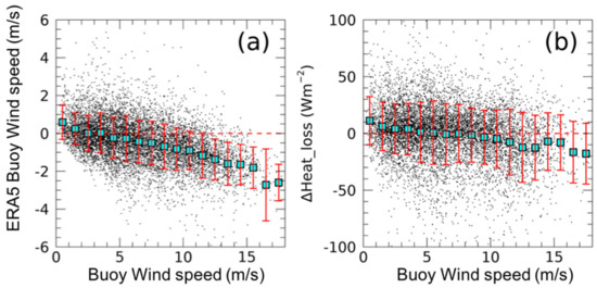
Figure 8.
ERA5 minus buoy wind speed (a) and ERA5 minus buoy heat loss (Latent + Sensible + net Longwave) as a function of the in situ measured wind speed (b). Averages and standard deviations over 1 m/s intervals are shown as blue squares and red bars, respectively.
The data we have in hand do not permit us to establish whether the discrepancies can be ascribed to a different quality of ERA5 reanalysis in the two regions or rather to the increased opportunity of maintenance of the instrumentation thanks to the vicinity to the small flat Lampedusa Island, where the ENEA research laboratory periodically operates the cleaning of the instruments.
On average, the use of ERA5 wind speed instead of in situ data in bulk formulae, produces an underestimation of the heat loss to the atmosphere of only 0.5 W/m2, nearly linearly varying from +11 W/m2 in calm conditions to −18 W/m2 for winds larger than 17 m/s (Figure 8b). The existence of a linear relationship between bias and wind speed was already reported for the ECMWF analysis and the ERA40 reanalysis [53]. Based on the analysis of one year of data acquired at four different sites in the Mediterranean Sea, it was shown that ECMWF analysis and ERA40 data underestimated the winds speed for values greater than about 10 m/s and 5 m/s respectively.
The impact of biases among the different estimates of the heat budget components on a numerical 1-D simulation (GOTM) of the near surface water temperature has been evaluated over a full seasonal cycle (4 April 2017 to 3 April 2018). When fluxes from measured meteorological data were used in the simulations, the modelled temperature values agreed very well with the in situ reference data: the bias was −0.1 °C when the model was run with in situ meteorological data and +0.1 °C when was run with ERA5 data (Figure 5 and Figure 7). However, more significant differences between in situ measurements and simulations were observed when GOTM was forced with other estimates of the flux components (prescribed fluxes): a mean overestimation of about 1 °C with respect to in situ measurements is observed when ERA5 fluxes were prescribed.
When in situ observations of the shortwave irradiance is used in the model instead of the ERA5 values, a good correspondence between modelled and measured water temperature is found over a relatively extended time interval (about a month), during which contribution from lateral advection may be considered negligible. When longwave irradiances are used, somewhat larger biases between modeled and measured temperatures are found. Very similar values of the total net heat budget, about 17 W/m2, are obtained with ERA5 fluxes and with ERA5 longwave radiation and turbulent fluxes and measured shortwave irradiance. The total net heat flux becomes about 34 W/m2 when in situ measurements of the longwave irradiance is used in the simulations. When ERA5 shortwave or longwave irradiances were substituted with the corresponding satellite measurements, annual mean biases increased in a range between 1.8 °C (shortwave from SEVIRI) and 3.5 °C (longwave from SEVIRI) and the total net heat flux varied between 22.9 and 40.4 W/m2. This result for SEVIRI’s data could be partially caused by the compensation of a bias in one flux term with another one, given that also the latent and sensible fluxes contribute to the total budget. To solve this question, satellite estimations of all flux components are needed. To date, only geostationary satellite data are provided with enough temporal resolution to resolve the diurnal cycle, excluding latitudes higher than 60 °N and 60 °S. In these high latitudes, only polar orbiting satellites can provide radiative flux data with enough time frequency due to intensified intersection of the swaths. The SEVIRI Downward Longwave Irradiance (DLI), however, is a bulk parameterization combining the ECMWF NWP model outputs and satellite derived cloud parameters and then cannot be considered a full satellite product, being the satellite contribution limited to the cloud cover determination (see http://www.osi-saf.org/lml/doc/osisaf_cdop3_ss1_atbd_geo_flx.pdf) (last accessed on 2 June 2021). On their hand, latent and sensible satellite heat flux determinations are mainly based on microwave data that empirically estimate meteorological variables, that in turn enter in the bulk formulae (for an example, see Algorithm Theoretical Basis Document HOAPS release 3.2 https://www.cmsaf.eu/SharedDocs/Literatur/document/2011/saf_cm_dwd_atbd_hoaps_1_1_pdf) (last accessed on 2 June 2021). This means that turbulent fluxes satellite estimates can suffer from the same problem of any equivalent determination based on bulk formulae.
Future microwave missions, such as Copernicus Imaging Microwave Radiometer (CIMR) and the Geostationary Interferometric Microwave Sounder (GIMS) [56] could provide data with daily, or even sub daily, frequencies, resolving the diurnal cycle on a global scale, potentially useful for turbulent heat flux estimates. CIMR will contribute to estimates of air–sea turbulent heat and moisture fluxes from simultaneous SST, wind speed, sea surface salinity, sea ice, rain rate and integrated cloud liquid water, opening a new era for unprecedented satellite applications.
Author Contributions
Conceptualization, S.M., J.P.; methodology, S.M., J.P., M.B., A.G.d.S., V.A., D.M., F.M., D.S., R.S.; formal analysis, S.M., J.P.; investigation, S.M., J.P., M.B., A.G.d.S., D.M., F.M., D.S., V.A., R.S.; writing-review and editing, S.M., J.P., M.B., A.G.d.S., D.M. All authors have read and agreed to the published version of the manuscript.
Funding
M.B. had a postdoctoral fellowship by the European Space Agency (ESA). This work was supported by the ESA Living Planet Fellowship Project PHYSIOGLOB: Assessing the inter-annual physiological response of phytoplankton to global warming using long-term satellite observations, 2018–2020. Measurements at Lampedusa and analyses have been also partially supported by the Marine Hazard Project, funded by the Italian Ministry for University and Research. J.P. acknowledges funding by the Copernicus Climate Change Service, Quality Assessment of ECV Products (C3S_511).
Institutional Review Board Statement
Not applicable.
Informed Consent Statement
Not applicable.
Data Availability Statement
The data presented in this study are available on request from the corresponding author.
Acknowledgments
J.P. expresses his gratitude to Lars Umlauf for hosting him at the Leibniz Institute for Baltic Sea Research at Warnemünde during a one-month sabbatical, in which advanced training on GOTM usage and turbulence modelling were unselfishly given. Elena Roget from the University of Girona is warmly thanked for providing trust, long term training on aquatic physics, financial support and scientific coordinates. Contributions by Fabrizio Anello, Carlo Bommarito, Tatiana Di Iorio, Giandomenico Pace and Salvatore Piacentino, who contributed to the Lampedusa Oceanographic Observatory operativity, are gratefully acknowledged This analysis has been supported and contributes also to the Project Marine Hazard, funded by the Italian Ministry for University and Research. The picture of Lampedusa in Figure 2 is image ISS024-E-10246, provided through the courtesy of the Earth Science and Remote Sensing Unit at NASA Johnson Space Center (and has been downloaded from http://eol.jsc.nasa.gov, accessed on 18 May 2021). Satellite and model reanalysis data were provided free of charge by EUMETSAT and ECMWF respectively. Four anonymous reviewers are thanked for their valuable contributions that helped to improve the quality of the manuscript.
Conflicts of Interest
The authors declare no conflict of interest.
References
- Myhre, G.; Shindell, D.; Pongratz, J. Anthropogenic and Natural Radiative Forcing. In Climate Change 2013: The Physical Science Basis Working Group I Contribution to the Fifth Assessment Report of the Intergovernmental Panel on Climate Change; Stocker, T., Ed.; Cambridge University Press: Cambridge, UK, 2014; pp. 659–740. [Google Scholar]
- Jordà, G.; Von Schuckmann, K.; Josey, S.A.; Caniaux, G.; García-Lafuente, J.; Sammartino, S.; Özsoy, E.; Polcher, J.; Notarstefano, G.; Poulain, P.M.; et al. The Mediterranean Sea heat and mass budgets: Estimates, uncertainties and perspectives. Prog. Oceanogr. 2017, 156, 174–208. [Google Scholar] [CrossRef]
- Millot, C. Another description of the Mediterranean Sea outflow. Prog. Oceanogr. 2009, 82, 101–124. [Google Scholar] [CrossRef]
- Garrett, C.; Outerbridge, R.; Thompson, K. Interannual Variability in Meterrancan Heat and Buoyancy Fluxes. J. Clim. 1993, 6, 900–910. [Google Scholar] [CrossRef]
- Castellari, S.; Pinardi, N.; Leaman, K. A model study of air–sea interactions in the Mediterranean Sea. J. Mar. Syst. 1998, 18, 89–114. [Google Scholar] [CrossRef]
- Bethoux, J. Budgets of the Mediterranean Sea-Their dependance on the local climate and on the characteristics of the Atlantic waters. Oceanol. Acta 1979, 2, 157–163. [Google Scholar]
- Bunker, A.; Charnock, H.; Goldsmith, R. A note on the heat balance of the Mediterranean and Red Seas. J. Mar. Res. 1982, 40, 73–84. [Google Scholar]
- Gilman, C.; Garrett, C. Heat flux parameterizations for the Mediterranean Sea: The role of atmospheric aerosols and constraints from the water budget. J. Geophys. Res. Ocean. 1994, 99, 5119–5134. [Google Scholar] [CrossRef]
- Matsoukas, C.; Banks, A.C.; Hatzianastassiou, N.; Pavlakis, K.G.; Hatzidimitriou, D.; Drakakis, E.; Stackhouse, P.W.; Vardavas, I. Seasonal heat budget of the Mediterranean Sea. J. Geophys. Res. Ocean. 2005, 110. [Google Scholar] [CrossRef]
- May, P. A Brief Explanation of Mediterranean Heat and Momentum Flux Calculations; Naval Oceanography Atmospheric Research Laboratory: Washington, DC, USA, 1986. [Google Scholar]
- Pettenuzzo, D.; Large, W.G.; Pinardi, N. On the corrections of ERA-40 surface flux products consistent with the Mediterranean heat and water budgets and the connection between basin surface total heat flux and NAO. J. Geophys. Res. Ocean. 2010, 115. [Google Scholar] [CrossRef]
- Ruiz, S.; Gomis, D.; Sotillo, M.G.; Josey, S.A. Characterization of surface heat fluxes in the Mediterranean Sea from a 44-year high-resolution atmospheric data set. Glob. Planet. Chang. 2008, 63, 258–274. [Google Scholar] [CrossRef]
- Criado-Aldeanueva, F.; Soto-Navarro, F.J.; García-Lafuente, J. Seasonal and interannual variability of surface heat and freshwater fluxes in the Mediterranean Sea: Budgets and exchange through the Strait of Gibraltar. Int. J. Climatol. 2012, 32, 286–302. [Google Scholar] [CrossRef]
- Smith, S.D.; Fairall, C.W.; Geernaert, G.L.; Hasse, L. Air-sea fluxes: 25 years of progress. Bound. Layer Meteorol. 1996, 78, 247–290. [Google Scholar] [CrossRef]
- Cronin, M.F.; Gentemann, C.L.; Edson, J.; Ueki, I.; Bourassa, M.; Brown, S.; Clayson, C.A.; Fairall, C.W.; Farrar, J.T.; Gille, S.T.; et al. Air-Sea Fluxes With a Focus on Heat and Momentum. Front. Mar. Sci. 2019, 6. [Google Scholar] [CrossRef]
- Pond, S.; Phelps, G.T.; Paquin, J.E.; McBean, G.; Stewart, R.W. Measurements of the Turbulent Fluxes of Momentum, Moisture and Sensible Heat over the Ocean. J. Atmos. Sci. 1971, 28, 901–917. [Google Scholar] [CrossRef][Green Version]
- Large, W.G.; Pond, S. Sensible and Latent Heat Flux Measurements over the Ocean. J. Phys. Oceanogr. 1982, 12, 464–482. [Google Scholar] [CrossRef]
- Moнин, A.; Oбyxoв, A. Ocнoвныe зaкoнoмepнocти тypбyлeнтнoгo пepeмeшивaния в пpизeмнoм cлoe aтмocφepы. Tp. гeoφиз. Ин-тa CCCP 1954, 151, 163–187. [Google Scholar]
- Garratt, J.R. Review of Drag Coefficients over Oceans and Continents. Mon. Weather Rev. 1977, 105, 915–929. [Google Scholar] [CrossRef]
- Fairall, C.W.; Bradley, E.F.; Rogers, D.P.; Edson, J.B.; Young, G.S. Bulk parameterization of air-sea fluxes for Tropical Ocean-Global Atmosphere Coupled-Ocean Atmosphere Response Experiment. J. Geophys. Res. Ocean. 1996, 101, 3747–3764. [Google Scholar] [CrossRef]
- Hill, R.J. Implications of Monin–Obukhov Similarity Theory for Scalar Quantities. J. Atmos. Sci. 1989, 46, 2236–2244. [Google Scholar] [CrossRef]
- Kondo, J. Air-sea bulk transfer coefficients in diabatic conditions. Bound. Layer Meteorol. 1975, 9, 91–112. [Google Scholar] [CrossRef]
- Kara, A.B.; Hurlburt, H.E.; Wallcraft, A.J. Stability-Dependent Exchange Coefficients for Air–Sea Fluxes. J. Atmos. Ocean. Technol. 2005, 22, 1080–1094. [Google Scholar] [CrossRef]
- Schiano, M.E.; Santoleri, R.; Bignami, F.; Leonardi, R.M.; Marullo, S.; Böhm, E. Air-sea interaction measurements in the west Mediterranean Sea during the Tyrrhenian Eddy Multi-Platform Observations Experiment. J. Geophys. Res. Ocean. 1993, 98, 2461–2474. [Google Scholar] [CrossRef]
- Bignami, F.; Marullo, S.; Santoleri, R.; Schiano, M.E. Longwave radiation budget in the Mediterranean Sea. J. Geophys. Res. Ocean. 1995, 100, 2501–2514. [Google Scholar] [CrossRef]
- Schiano, M.E. Insolation over the western Mediterranean Sea: A comparison of direct measurements and Reed’s formula. J. Geophys. Res. Ocean. 1996, 101, 3831–3838. [Google Scholar] [CrossRef]
- Reed, R.K. On Estimating Insolation over the Ocean. J. Phys. Oceanogr. 1977, 7, 482–485. [Google Scholar] [CrossRef]
- Simpson, J.J.; Paulson, C.A. Mid-ocean observations of atmospheric radiation. Q. J. R. Meteorol. Soc. 1979, 105, 487–502. [Google Scholar] [CrossRef]
- Rosati, A.; Miyakoda, K. A General Circulation Model for Upper Ocean Simulation. J. Phys. Oceanogr. 1988, 18, 1601–1626. [Google Scholar] [CrossRef]
- Brunt, D. Notes on radiation in the atmosphere. I. Q. J. R. Meteorol. Soc. 1932, 58, 389–420. [Google Scholar] [CrossRef]
- Anderson, E.R. Energy-budget studies. Water-Loss Investigation: Lake Hefner Studies; Technical Report; United States Geological Survey: Washington, DC, USA, 1954; Volume 269, pp. 71–119. [Google Scholar] [CrossRef]
- Berliand, M.; Berliand, T. Measurement of the effective radiation of the Earth with varying cloud amounts. Izv. Akad. Nauk SSSR Ser. Geofiz 1952, 1, 64–78. [Google Scholar]
- Swinbank, W.C. Long-wave radiation from clear skies. Q. J. R. Meteorol. Soc. 1963, 89, 339–348. [Google Scholar] [CrossRef]
- Efimova, N. On methods of calculating monthly values of net longwave radiation. Meterol. Gidrol. 1961, 10, 28–33. [Google Scholar]
- Clark, N.; Eber, L.E.; Laurs, R.M.; Renneer, J.; Saur, J. Heat Exchange between Ocean and Atmosphere in the Eastern North. Pacific for 1961-71; Technical Report NMFS SSRF-682; NOAA: Seattle, WA, USA, 1974. [Google Scholar]
- Hastenrath, S. Heat Budget Atlas of the Tropical Atlantic and Eastern Pacific Oceans; University of Wisconsin Press: Madison, WI, USA, 1978. [Google Scholar]
- Pinardi, N.; Allen, I.; Demirov, E.; De Mey, P.; Korres, G.; Lascaratos, A.; Le Traon, P.Y.; Maillard, C.; Manzella, G.; Tziavos, C. The Mediterranean ocean forecasting system: First phase of implementation (1998–2001). Ann. Geophys. 2003, 21, 3–20. [Google Scholar] [CrossRef]
- Madec, G.; Bourdallé-Badie, R.; Bouttier, P.-A.; Bricaud, C.; Bruciaferri, D.; Calvert, D.; Chanut, J.; Clementi, E.; Coward, A.; Delrosso, D.; et al. NEMO Ocean Engine; Note du Pôle de Modélisation, Institut Pierre-Simon Laplace (IPSL): Guyancourt, France, 2017; No 27. [Google Scholar]
- Liguori, G.; Di Lorenzo, E.; Cabos, W. A multi-model ensemble view of winter heat flux dynamics and the dipole mode in the Mediterranean Sea. Clim. Dyn. 2017, 48, 1089–1108. [Google Scholar] [CrossRef]
- Karagali, I.; Høyer, J.L.; Donlon, C.J. Using a 1-D model to reproduce the diurnal variability of SST. J. Geophys. Res. Ocean. 2017, 122, 2945–2959. [Google Scholar] [CrossRef]
- Babar, B.; Graversen, R.; Boström, T. Solar radiation estimation at high latitudes: Assessment of the CMSAF databases, ASR and ERA5. Sol. Energy 2019, 182, 397–411. [Google Scholar] [CrossRef]
- Luo, B.; Minnett, P.J.; Szczodrak, M.; Nalli, N.R.; Morris, V.R. Accuracy Assessment of MERRA-2 and ERA-Interim Sea Surface Temperature, Air Temperature, and Humidity Profiles over the Atlantic Ocean Using AEROSE Measurements. J. Clim. 2020, 33, 6889–6909. [Google Scholar] [CrossRef]
- Trolliet, M.; Walawender, J.P.; Bourlès, B.; Boilley, A.; Trentmann, J.; Blanc, P.; Lefèvre, M.; Wald, L. Downwelling surface solar irradiance in the tropical Atlantic Ocean: A comparison of re-analyses and satellite-derived data sets to PIRATA measurements. Ocean. Sci. 2018, 14, 1021–1056. [Google Scholar] [CrossRef]
- Renfrew, I.A.; Barrell, C.; Elvidge, A.D.; Brooke, J.K.; Duscha, C.; King, J.C.; Kristiansen, J.; Cope, T.L.; Moore, G.W.K.; Pickart, R.S.; et al. An evaluation of surface meteorology and fluxes over the Iceland and Greenland Seas in ERA5 reanalysis: The impact of sea ice distribution. Q. J. R. Meteorol. Soc. 2021, 147, 691–712. [Google Scholar] [CrossRef]
- Belmonte Rivas, M.; Stoffelen, A. Characterizing ERA-Interim and ERA5 surface wind biases using ASCAT. Ocean. Sci. 2019, 15, 831–852. [Google Scholar] [CrossRef]
- Di Sarra, A.; Bommarito, C.; Anello, F.; Di Iorio, T.; Meloni, D.; Monteleone, F.; Pace, G.; Piacentino, S.; Sferlazzo, D. Assessing the Quality of Shortwave and Longwave Irradiance Observations over the Ocean: One Year of High-Time-Resolution Measurements at the Lampedusa Oceanographic Observatory. J. Atmos. Ocean. Technol. 2019, 36, 2383–2400. [Google Scholar] [CrossRef]
- Meloni, D.; Di Biagio, C.; di Sarra, A.; Monteleone, F.; Pace, G.; Sferlazzo, D.M. Accounting for the Solar Radiation Influence on Downward Longwave Irradiance Measurements by Pyrgeometers. J. Atmos. Ocean. Technol. 2012, 29, 1629–1643. [Google Scholar] [CrossRef]
- Frouin, R.; Chertock, B. A Technique for Global Monitoring of Net Solar Irradiance at the Ocean Surface. Part I: Model. J. Appl. Meteorol. Climatol. 1992, 31, 1056–1066. [Google Scholar] [CrossRef]
- Brisson, A.; Le Borgne, P.; Marsouin, A. Development of algorithms for surface solar irradiance retrieval at O&SI SAF low and mid latitudes. Eumetsat Ocean. and Sea Ice SAF Internal Project Team Report; Eumetsat: Darmstadt, Germany, 1999; Volume 69, pp. 71–73. [Google Scholar]
- Burchard, H.; Bolding, K.; Ruiz-Villarreal, M. GOTM, a General Ocean Turbulence Model. Theory, Implementation and Test Cases; Technical Report EUR 18745; Joint Research Centre, European Commission: Ispra, Italy, 1999. [Google Scholar]
- Umlauf, L.; Burchard, H. Second-order turbulence closure models for geophysical boundary layers. A review of recent work. Cont. Shelf Res. 2005, 25, 795–827. [Google Scholar] [CrossRef]
- Burchard, H.; Bolding, K. Comparative Analysis of Four Second-Moment Turbulence Closure Models for the Oceanic Mixed Layer. J. Phys. Oceanogr. 2001, 31, 1943–1968. [Google Scholar] [CrossRef]
- Ruti, P.M.; Marullo, S.; D’Ortenzio, F.; Tremant, M. Comparison of analyzed and measured wind speeds in the perspective of oceanic simulations over the Mediterranean basin: Analyses, QuikSCAT and buoy data. J. Mar. Syst. 2008, 70, 33–48. [Google Scholar] [CrossRef]
- Jerlov, N. Optical Oceanography; Elsevier Publishing Company: Amsterdam, The Netherlands; London, UK; New York, NY, USA, 1968; Volume 5. [Google Scholar]
- Payne, R.E. Albedo of the Sea Surface. J. Atmos. Sci. 1972, 29, 959–970. [Google Scholar] [CrossRef]
- Liu, H.; Wu, J.; Zhang, S.; Yan, J.; Niu, L.; Zhang, C.; Sun, W.; Li, H.; Li, B. The Geostationary Interferometric Microwave Sounder (GIMS): Instrument overview and recent progress. In Proceedings of the 2011 IEEE International Geoscience and Remote Sensing Symposium, Vancouver, BC, Canada, 24–29 July 2011; pp. 3629–3632. [Google Scholar]


Publisher’s Note: MDPI stays neutral with regard to jurisdictional claims in published maps and institutional affiliations. |
© 2021 by the authors. Licensee MDPI, Basel, Switzerland. This article is an open access article distributed under the terms and conditions of the Creative Commons Attribution (CC BY) license (https://creativecommons.org/licenses/by/4.0/).