1. Introduction
The demand for sustainable food production continues to increase due to population growth, particularly in the developing world [
1]. Stable global food production is threatened by changing and increasingly volatile environmental conditions in food growing regions [
2,
3]. Breeding crop varieties that have both high yields and resilience to abiotic stress has the potential to overcome these challenges to global food production and stability [
4]. New, data-driven techniques for crop breeding require large amounts of genomic and phenomic information [
5]. However, traditional plant phenotyping methods are slow, destructive and laborious [
6]. Image-based plant phenotyping has the potential to increase the speed and reliability of phenotyping by using remote sensing technology, such as unmanned aerial vehicles (UAVs), to estimate phenomic information from field crop breeding experiments [
7,
8,
9,
10,
11]. UAVs can monitor a large field in a relatively short period of time with different imaging payloads including RGB, multispectral, hyperspectral, and thermal cameras [
12,
13,
14,
15]. UAV images can, in turn, be analyzed to estimate phenotypic traits, such as vegetation, flowering and canopy temperature [
16,
17,
18,
19].
For applications in crop breeding, detailed phenotypic information is often required, such as counting the number of seedlings or plant organs within a small region of a field experiment. In order to adequately capture and estimate these fine plant features, images with high spatial resolution are required. For example, previous work has demonstrated that low spatial image resolution has a substantial negative effect on the accuracy of measuring plant ground cover from images [
20]. Extracting textural features from aerial images for vegetation classification also requires high spatial resolution [
21]. It has also been shown that the accuracy of detecting and localizing objects in images is highly dependent on image resolution [
22,
23]. The requirement of high spatial image resolution poses a challenge for UAV imaging, because a number of factors limit the resolution of UAV-acquired images.
The resolution of aerial imaging is directly associated with several factors including the camera sensor’s resolution, the camera lens’ focal length, and the altitude of the UAV flight [
24]. A smaller ground sampling distance (GSD), representing a higher spatial resolution, requires lower altitude (shorter distance between the camera and target being imaged), a higher resolution sensor, and/or a longer focal length lens. However, these variables have trade-offs that limit GSD in practice. UAVs are often flown at a high altitude or with a shorter focal length lens, in order to capture the entire field in a short period of time, due to limited battery life [
25]. High-resolution sensors are expensive and heavier and must be flown on larger and more expensive UAVs with higher payload capacity. For crop imaging, multispectral sensors are often used, which is the trade-off spatial resolution for spectral resolution [
21]. Even if a small GSD is obtained by optimizing sensor and flight parameters, during a flight, atmospheric disturbances and wind can cause image blur and substantially reduce the effective spatial resolution of the acquired images. Managing the tradeoffs between cost and image fidelity forces potentially unpalatable compromises on those monitoring crops.
An alternative to achieving high spatial resolution aerial images is enhancing the details of aerial images algorithmically. Image super resolution is a promising approach for reconstructing a high-resolution (HR) image from its low-resolution (LR) counterpart to improve the image detail. This has an obvious benefit, as finer grained imagery can be derived from lower cost, lighter-weight cameras, allowing smaller, less expensive UAVs to be employed. In an agricultural context, image super resolution could be used to convert LR images to HR images, improving image details for phenotyping tasks such as flower counting. Image super resolution is a challenging problem and an active area of computer vision research. Deep learning-based methods have shown potential to enhance the robustness of traditional image super resolution techniques [
26,
27,
28]. However, most of the state-of-the-art models were evaluated over public datasets consisting of urban scenes, animals, objects and people [
29,
30]. While a few studies have applied super resolution methods to plant images, these have been conducted with close-up images of fruit [
31] or leaves [
32,
33]. It is not clear how well super resolution methods would work when applied to aerial images of agricultural fields that include substantial high frequency content and highly self-similar plants within the same spatial region of the field.
Because almost all super resolution methods are tested with synthetic data—datasets where HR images are downsampled with a known kernel (e.g., bicubic interpolation) to obtain LR/HR image pairs—the actual performance of super resolution in practice is also uncertain. A few datasets have been proposed with paired real-world LR and HR images by capturing the same static scene with the same sensor with different focal lengths [
34] or with two side-by-side sensors with different focal lengths [
35]. Recently, the NTIRE 2020 dataset has been proposed for real-world super resolution with smart phone images [
36]. However, a paired LR/HR image dataset of aerial images does not currently exist, and is more challenging to collect, as it requires capturing both LR and HR images of a dynamic scene.
In this paper, we address these shortcomings by providing a paired drone image set of low and high resolution images, and characterize the performance against state of the art super resolution algorithms to establish the utility of super resolution approaches in agriculture, and more generally for other applications from drone images. We provide a new real-world dataset of LR/HR images collected by co-mounting LR and HR sensors on the same UAV. We evaluate the performance of three deep learning-based super resolution models against the collected data. We evaluate how well a model trained with synthetic data generalizes to real-world LR images. The contributions of this study include:
A novel dataset of paired LR/HR aerial images of agricultural crops, employing two different sensors co-mounted on a UAV. The dataset consists of paired images of canola, wheat and lentil crops from early to late growing seasons.
A fully automated image processing pipeline for images captured by co-mounted sensors on a UAV. The algorithm provides image matching with maximum spatial overlap, sensor data radiometric calibration and pixel-wise image alignment to contribute a paired real-world LR and HR dataset, essential for curating other UAV-based datasets.
Extensive quantitative and qualitative evaluations across three different experiments including training and testing super resolution models with synthetic and real-world images to evaluate the efficacy of real-world dataset in a more accurate analysis of image-based plant phenotyping.
2. Background and Related Work
High spatial resolution images are important for computer vision tasks when fine details about the original scene are required [
37]. In remote sensing, the pixel size of aerial images matters because it impacts the accuracy of image analysis [
20]. There are usually a variety of ground objects in the sensor’s field of view, where a pixel in a remote sensing image may contain a mixture of ground objects information, called mixed pixel. This can impact information extraction, such as image classification and object detection in mixed pixels [
38].
Coarse spatial resolution is likely to increase the number of mixed pixels in aerial images, where the major proportion of the objects existing in a mixed pixel determine the identity of ground objects [
39]. To some extent, spectral unmixing can handle the identity of mixed pixels, but it cannot provide spatial distribution information for remote sensing images [
40]. The super resolution approach is a process of improving details within an image, predicting finer spatial resolution, especially where the details are essentially unknown to reduce the spatial uncertainty in output images. A finer spatial resolution results in smaller pixel sizes and fewer mixed pixels in an image [
41].
Super resolution is a classic problem in computer vision, and generally there are many possible upsampling solutions for a given low resolution image. Machine learning or image processing approaches have suggested different complimentary solutions including traditional methods, and deep learning-based algorithms to increase the visual resolution of an image.
2.1. Traditional Super Resolution Methods
The simplest way to provide a super-resolved image is to apply an interpolation filter on sample image by amplifying existing high-frequency information in the image. However, real-world images do not contain severe high-frequency information, meaning that the algorithm would likely create a blurred output [
42].
Generating an HR image from a sequence of LR images taken from the same scene is referred to as multi-image super resolution (MISR). This approach works using iterative back projection, where a set of LR images are registered to reconstruct a single HR image by aggregating LR images. MISR can be compromised by registration errors, if the resolution of the original images is not sufficient to observe fine features, or the number of unknown samples is large, which can result in substantial computational costs [
43].
Single image super resolution (SISR) refers to the task of restoring an HR image from a single LR image, requiring image priors. The core idea of learning-based SISR methods is to learn the mapping between the LR and HR images. This approach predicts the missing high frequency information that does not exist in the LR image and which cannot be reconstructed by simple image interpolation [
44]. SISR is more general than MISR because there are fundamental limits to MISR, such as poor registration, low resolution gain, too much noise, and slow processing speed that deter MISR approach to provide higher resolutions [
45].
2.2. Example-Based Super Resolution
The most successful alternative to interpolation and MISR is example-based super resolution with machine learning. Example-based approaches include parametric methods [
46] and non-parametric methods [
47], which typically build upon existing machine learning techniques. Parametric methods create the super resolution image via mapping functions, controlled by a compact number of parameters, learned from examples that do not necessarily come from the input image. One possible solution is to adapt the interpolation algorithm to the local covariances images [
45].
The introduction of the latest machine learning approaches made substantial improvements in non-parametric models in terms of accuracy and efficiency. Non-parametric methods can, in turn, be classified as internal or external learning methods [
48].
Internal learning models sample patches obtained directly from the input image. These patches are extracted from the self-similarity property of natural images [
49], such that the smallest patches in a natural image are likely to be observed in the down-scaled version of the same image [
50,
51]. External super resolution methods use a common set of images to predict missing information, especially high frequency data from a large and representative set of external pairs of images. Numerous super resolution methods used paired LR-HR images, collected from external databases. External super resolution papers generally used supervised learning methods, including nearest neighbor [
44], and sparse coding [
52,
53,
54,
55,
55].
2.3. Deep Learning-Based Super Resolution
Deep learning techniques have the potential to improve the robustness of traditional image super resolution methods and reconstruct higher quality images in various scales. Many deep learning-based networks achieve significant performance on SISR, employing a synthetic LR image as input for the super resolution model. Some models use predefined interpolation as the upsampling operator to produce an intermediate image with the desired size and feed that image into the network for further refinement [
56]. Residual learning and recursive layers were further employed in this framework to enhance image quality [
57,
58].
Single upsampling frameworks offer an effective solution to increase the spatial resolution at the end of the learning process while learning the mapping in the LR space without a predefined operator [
59,
60], where residual learning helps to exploit fine features in the LR space [
27,
61,
62]. Progressive upsampling gradually reconstructs HR images, allowing the network to first discover the actual scale structure of the LR image and then predict finer scale details [
26]. An iterative up and downsampling framework increases the learning capacity employing concatenation operator [
28].
Several different super resolution strategies have been proposed to enhance the quality of real-world images, because the performance of learning-based super resolution drops when the kernel deviates from the true kernel [
63]. Most super resolution models which estimate the true kernel involve complex optimization procedures [
64,
65,
66,
67,
68,
69]. Deep learning is an alternative strategy for estimating the true kernel for real-world image super resolution [
70,
71,
72]. Deep learning-based models assume that the degradation kernels are not available and attempt to estimate the optimal kernel, either using self-similarity properties [
64,
70,
71] or adapting an alternating optimization algorithm [
63,
73]. These models have shown promising results in up to
image super resolution.
2.4. Image Pre-Processing for Raw Data
Raw image processing employs raw sensor data to enhance the image quality for computer vision tasks. A maximum a posteriori method was proposed to jointly stitch and super resolve multi-frame raw sensor data [
74]. A deep learning-based model was employed for demosaicing and denoising simultaneously [
75]. A similar work was proposed to denoise a sequence of synthetic raw data [
76]. An end-to-end deep residual network was proposed to learn mapping between raw images and targets to recover in high-quality images [
77]. In [
78], a learning-based pipeline was introduced to process low-light raw images with their corresponding reference images in an end-to-end fashion.
3. Materials and Methods
In this section, we introduce our aerial image dataset, detail the image pre-processing steps used to obtain paired LR/HR images, and describe the experiments for evaluating super resolution models with the datatset.
3.1. Dataset Collection
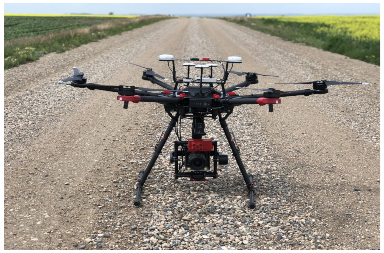
For training with real-world images, we collected original datasets consisting of raw LR and HR images, captured by two separate sensors co-mounted on a UAV, visualized in
Figure 1. As the two sensors have different configurations such as discrepancies in capture rate, different spectral bands, and different fields of view, we first need to match images with the maximum overlap of the same scene, calibrate images radiometrically, and align the calibrated images pixel-wise with a registration algorithm. The created dataset enables training a model in an end-to-end fashion to jointly deblur and super resolve the real-world LR images. Our dataset will be made publicly available to encourage the development of computer vision methods for agricultural imaging and help enable next generation image-based plant phenotyping for accurate measurement of plants and plant organs from aerial images.
To create our dataset, we obtain aerial images of the entirety of three breeding field trials of canola, lentil and wheat crops employing two different sensors. The lentil and wheat fields are located side by side, which are captured together during the same flight. The number of images in the lentil and wheat datasets is low, because the flight period used to capture these two fields is equivalent to the time spent on the canola field due to limited battery life. The canola image acquisition experiment was conducted at the Agriculture and Agri-Food Canada Research Farm near Saskatoon (52.181196 °N, −106.501494 °E), SK, and the lentil and wheat image acquisition experiment was conducted at Nasser location (52.163455 °N, −106.515038°E) of Kernen Crop Research Farm, Saskatoon, SK in Canada.
The images were acquired over an entire growing season ranging from early, mid to late growth stages over the three fields in 2018. The canola dataset contains images from both 2018 and 2019 growing seasons.
Table 1 shows the diversity of growth stages in each dataset related to the captured date and the number of images in each date. The total number of matched images in the canola and in the lentil and wheat datasets are 1201 and 416 images, respectively. As the lentil and wheat datasets were captured together during a single flight, we keep these two datasets together in
Table 1, because the calibrated panel reflection (CRP) required to match the LR and HR images based on their relative timestamp, is merely captured once during a flight. To match the LR and HR images pair-wise, we need to obtain the capture time of CRP’s image via its metadata (
Figure 2). The numbers of the lentil and wheat images are individually 210 and 206 images respectively, shown, as in total, 416 images in
Table 1. The lentil and wheat datasets will be separated later for further analysis when training and testing the models.
Each dataset covers a diverse range of genotypes. The canola field has 56 varieties of canola, such that substantial variations exist in appearance in the dataset. The wheat field contains 17 varieties in microplots, while the lentil field has 16 varieties in microplots. The wheat or lentil trial has 47 rows and 12 columns of microplots in three aligned blocks. The spacing between rows within a plot in the canola trial and in the lentil and wheat trials were approximately 0.3 m and 0.6 m, respectively. Low sowing density was observed in the lentil field and normal sowing density in the canola and wheat fields [
79,
80].
For capturing low resolution images, we used the Micasense Rededge camera, a widely used multispectral (5-band) camera for monitoring crops. For capturing high resolution images, we used the Phase One IXU-1000 camera, a high-end medium format RGB camera generally used for commercial purposes. Both cameras were mounted to an Ronin-MX gimbal on a DJI Matrice 600 UAV and captured images simultaneously during the flight. Canola images were captured with the UAV at 20 m altitude, and the lentil and wheat fields were captured from 30 m above the ground. The two sensors are substantially different in their configurations, summarized in
Table 2, when the two sensors are at the same altitude about 20 m. For example, LR images represent a smaller area of the field than HR images, because the Phase One IXU-1000 sensor has a wider field of view. At a 20 m flight altitude, the GSD between the two sensors was 1.7 mm/pixel and 12.21 mm/pixel respectively, which represents a significant difference in spatial resolution, meaning small detailed information is missing in the LR images.
Multispectral imaging devices generally measure the energy and light emissions from the surrounding environment. The Micasense Rededge multispectral sensor uses a downwelling light sensor (DLS) in conjunction with MicaSense Rededge’s CRP. To compensate for the illumination conditions during the flight, CRP images are usually captured before or after each flight. The panel image provides a precise representation of the amount of light variations during the flight and on the ground at the time of capture. This helps to enhance reflectance estimates in situations where the surrounding illumination conditions are changing. This situation requires a conversion to normalized reflectance [
81].
3.2. Image Pre-Processing
During data collection, the two sensors were not synchronized for every frame, meaning images may not be perfectly matched. In addition, the separate spectral sensors of the LR camera require color calibration to obtain a unitless RGB image. Therefore, the following pre-processing steps were performed to create the paired LR/HR dataset for super resolution model training: (1) match LR and HR images with sufficient spatial overlap, (2) correct LR images using at-surface reflectance conversion; and (3) employ a registration algorithm for pixel-wise alignment between LR and HR images.
3.2.1. Image Matching
As the two sensors were not synchronized during flight, we first need to find closely matching LR and HR pairs based on their relative timestamp. To pair training images, we extract the metadata from images of the CRP captured by the two sensors simultaneously. The metadata Original DateTime of the two images are parsed to acquire the time difference between the two sensors, enabling the computation of a threshold value used for matching images with maximum spatial overlap.
Figure 2 formally describes the image matching process between LR and HR images, while calibrating the LR images radiometrically.
3.2.2. Radiometric Calibration
The Micasense Rededge sensor has been equipped with a DLS to measure the incident light, because images do not typically provide a uniform radiometric response due to atmospheric disturbances. To utilize the image information in quantitative analysis, the data need to be radiometrically calibrated.
Reflectance measurement in passive imaging is influenced by illumination condition, scattering light in the atmosphere, surrounding environment, the spectral and directional reflectance of an object, and the object’s topography [
82]. We used the proscribed process for the Micasense Rededge [
83] to convert raw multispectral pixels to radiance and then to reflectance as unitless images. To convert raw pixels into reflectance, an image of the CRP is obtained before the flight, which is used for the raw LR images calibration radiometrically. To determine the transfer function from raw pixels to reflectance for the
ith band of the multispectral image:
where
denotes the calibrated reflectance factor for band
i.
represents the average reflectance of the CRP for the
ith band.
represents the average value of the radiance for pixels inside the panel for the
ith band.
The workflow includes compensations for sensor black-level, sensor sensitivity, sensor gain and exposure settings, and vignette effects of the lens. All of the required parameters were obtained from metadata information inside the raw LR images.
In multispectral captures, each band must be aligned with other bands to represent meaningful data. To do this, all of the min and max values over all five channels are adjusted to the minimum and maximum range of all channels. When the transformation is completed, the final image appears in true color.
3.2.3. Multi-Sensor Image Registration
The LR and HR images require to be aligned, where every pixel of the LR image corresponds to a group of pixels of the HR image. As the field of view of the two sensors is dissimilar, pixel-wise alignment is required between the LR and HR datasets. We employ the scale invariant feature transform (SIFT) registration algorithm to perform this task [
84].
For image registration, we use matched and radiometrically calibrated images. First, we register multispectral images over different bands, because multispectral sensors cause spatial misalignment between different bands. We followed a traditional approach for multispectral image registration, in which we set a band as a reference and align the other bands accordingly [
85]. Second, we register the HR image with its corresponding aligned RGB LR image. For an accurate pixel-wise registration, we alternate between the LR and HR images. We first resize the LR image to the size of the HR image and then designate the LR image as a reference image and align the HR image accordingly. We chose the LR image as reference because the field of view of the HR sensor is wider. We perform another registration, resizing the HR image obtained from the first alignment phase to the original size of the LR image and hold the HR images as reference and align the LR image accordingly.
Figure 3 demonstrates samples of the raw and aligned images existing in our dataset. Small number of paired images in our dataset have oblique view that have not been discarded, because they do not impact the process of training and testing of super resolution models.
Our crafted dataset consists of paired images where the scale of the LR and HR images is not a fixed factor. The size of the raw LR images per band and raw HR images are respectively (960, 1280) and (8708, 11,608, 3), such that the HR image is approximately 9× larger than the LR counterpart. The proposed image pre-processing pipeline can process LR and HR images in their actual sizes for registration. However, in this work, we employed cropped images for image registration to avoid costly computations and memory overload.
We randomly crop the red, green and blue bands of the LR sensor to pixels and align all three bands pixel-wise to create an RGB composite. We crop the corresponding region from the HR counterpart and align the LR and HR images pixel-wise. After pixel-wise image registration, the HR images are approximately larger in height and width, because the Phase One IXU-1000 sensor has wider field of view and some features are cut off in co-registered images such that the scale size between the aligned LR and HR images is roughly .
We then resized the HR images using bicubic interpolation to create an exact larger HR image than the LR counterpart to facilitate training. If the number of keypoints between the two images during image registration is less than 10 (the default number used by the SIFT algorithm), our algorithm skips those images and moves to the next pair.
To create our dataset, we cropped only one patch out of each LR and HR image during image registration. The proposed algorithm has the capacity to extract more patches from one image. One patch per image was used to reduce computational time.
We employ our dataset to train and test an
super resolution model. After image registration, we obtain a dataset consisting of 1581 paired images, including lentil, wheat and canola crops. We split the lentil and wheat dataset to analyse each dataset individually. There are 198 paired images in the lentil, 197 paired images in the wheat, and 1186 paired images in the canola dataset. The number of total paired images in each dataset is slightly different from matched numbers reported in
Table 1, because we used random uniform cropping over the LR and HR images for image registration and the automated algorithm skips images where there are no sufficient keypoints, especially in patches with most ground view. The number of paired images may change between runs of the algorithm due to different cropped regions. We also have a dataset combining the three crops called a three-crop dataset.
3.3. Experiments
We evaluated three deep learning-based super resolution models using our dataset. We focus on three different experiments, including synthetic-synthetic, synthetic-real, and real-real strategies to evaluate the performance of each model across real-world images.
3.3.1. Model Selection
Several different models have been introduced to super resolve real-world LR images [
63,
70,
71]. These models have demonstrated promising results for
super resolution. For an
image super resolution, we employ three state-of-the-art SISR baseline models, including LapSRN [
26], SAN [
27], and DBPN [
28], along with bicubic interpolation.
LapSRN [
26] is built upon pyramid blocks to learn feature mapping progressively at
levels, where
M is the scaling factor. A progressive upsampling architecture tries to decompose a difficult task into simple tasks to reduce the learning difficulty, especially for larger scaling factors in image super resolution. At each stage, the images are upsampled to an intermediate higher spatial resolution used as input for the subsequent modules.
SAN [
27] is a direct learning model which learns salient representations in LR space and upsamples images into desired size via the last convolutional layer to improve computational efficacy. A second-order attention block was employed to learn the spatial correlations of features and improve feature expression.
DBPN [
28] leverages the back projection algorithm to capture the feature dependencies between LR and HR pairs. This framework employs up and downsampling layers iteratively and reconstructs the HR image resulting from all intermediate connections. The iterative back projection algorithm helps to compute the reconstruction error based on the connections between the LR and HR spaces and fuse it back to the network to enhance the quality of reconstructed images.
These models were selected as representatives of their respective architectures. All these models have achieved results that are near the state-of-the-art on benchmark datasets, such as BDS100 [
86], Set5 [
49], Set14 [
55], Urban100 [
29], and Manga109 [
87], reported in [
26,
27,
28]. Bicubic interpolation was chosen to provide a baseline for comparison.
3.3.2. Experimental Setup
To test the efficacy of the state-of-the-art super resolution models on aerial crop images, we conduct three experiments to evaluate whether or not using real-world images is needed, or if training with synthetic LR, downsampled HR images, is sufficient.
Experiment 1: Synthetic-Synthetic
In the synthetic-synthetic experiment, we train and test the models on synthetic data, where the LR images are obtained by downsampling HR images via bicubic interpolation. A random patch of the HR image was downsampled to . The downsampled image is used as input for the models. The kernel used in the LR image is therefore known. At inference, we compare the performance of the trained models in the same fashion of training, but with larger patches of size downsampled to as input. This experiment is meant to provide an approximate upper bound on the performance of the algorithms, because it solves the simpler known kernel problem.
Experiment 2: Synthetic-Real
In the synthetic-real experiment, we train the models using synthetic data, but then test the models using real-world LR images in our dataset. At inference, we employ a patch of our real-world LR image as input. The output is an image with the size of . This strategy employs a known kernel problem during training, but the unknown kernel problem at inference, and allows us to evaluate how well models trained on synthetic data generalize to unseen real-world LR images.
Experiment 3: Real-Real
In the real-real experiment, we train and test the models on real-world LR/HR images in our dataset. We employ a random patch of the real-world LR image and its corresponding patch from the real-world HR dataset with the size of as input and target, respectively during training. At inference, a patch of the real-world LR image is used as input to be upsampled and reaches a size of . For both training and testing, the kernel is not known, therefore we are solving an unknown kernel problem.
3.3.3. Model Training
We train all models on our dataset from scratch without employing pretrained models. We defined two input pipelines for reading either synthetic or real-world images. For the input pipeline of synthetic images, we only use HR images and their downsampled samples for training or testing the models. For the input pipeline of real-world images, we need to find the corresponding regions between the LR and HR images, where the HR images are approximately larger than their LR counterpart.
We crop one patch per image during the training and testing of all models. We train the models with stochastic cropped images to enhance the models’ performances, however, we require the same patches over all models at inference to evaluate the performance of the models equivalently.
We use
of each dataset for training and
as a test set. Here, we again crop one patch per image during training and testing. The input data are normalized to
. Data augmentation is performed by randomly rotating and horizontally flipping the input. The Adam solver [
88] with the default parameters
is employed to optimize the network parameters. The learning rate is set at
for all models and is decayed linearly. All models are trained for 200 epochs.
3.3.4. Evaluation Measures
To evaluate the performance of the super resolution models, we employ three standard measures, including structural similarity index (SSIM) [
89] and peak signal-to-noise ratio (PSNR) [
90] used in many super resolution tasks along with the dice similarity coefficient (DSC) [
91] to assess segmentation accuracy. SSIM measures the perceived quality of the reconstructed image, based on a distortion-free reference image. The human visual system is likely adapted to image structures [
92]. SSIM measures the structural similarity between images based on luminance, contrast, and structures’ comparisons [
89]. Higher SSIM value represents how well the high frequency information in an image was preserved. PSNR expresses the ratio between the maximum possible power of the reference image and the power of the reconstructed image that influences the quality of image representation. PSNR measures the pixel-level differences between the reconstructed and reference images instead of visual perception. Consequently, it often indicates lower performance in the reconstructed images of real scenes [
90]. Higher PSNR means that more noise was removed from an image. DSC measures the similarity between two images to express the spatial overlap between two segmented regions. Higher DSC represents a larger overlap between the two segmented regions.
To evaluate the image quality in terms of SSIM and PSNR at inference, we transform the reconstructed and target images into YCbCr colorspace. This conversion is more effective in pixel intensity evaluation and object definition compared to RGB, because YCbCr benefits from components separation that enables lower resolution capability of human visual system for color detection with respect to luminosity [
93].
In addition to standard image metrics, we also evaluate metrics specifically relevant for plant phenotyping: flower segmentation and excess green index [
94] commonly used for agricultural purposes. In plant breeding, flowering is an important phenotype that expresses the potential of yield in plants [
95].
For flower segmentation, we transform RGB images to Lab colorspace and employ Otsu’s thresholding [
96] to segment flowers in both reconstructed and target images [
97]. DSC is applied over the two segmented images. Vegetation identification from outdoor imagery is an important step in evaluating crop’s vigour, vegetation coverage, and growth dynamics [
16]. Excess green index [
94] provides a grey scale image, outlining a plant region of interest following:
where
g,
r,
b represent green, red and blue bands respectively. The grey scale image plays a role of a mask to segment the entire image. DSC [
91] is used as a segmentation measure between the two segmented images.
4. Results
In this section, we evaluate the performance of the super resolution models trained and tested with each individual experiment. To demonstrate the efficacy of real-world images, we have shown extensive quantitative and qualitative analysis across each individual experiment, employing both standard and domain specific measures.
We evaluate the performance of super resolution models on our dataset, employing the synthetic-synthetic, synthetic-real, and real-real experiments.
Table 3 and
Table 4 represent the performance of the models over the PSNR and SSIM values. In the synthetic-synthetic experiment, deep learning models were able to reconstruct reasonable quality images for the canola and three-crop datasets, but they did not outperform the bicubic interpolation for the lentil and wheat datasets. The results for the synthetic-real experiment indicate that the super resolution models cannot generalize to unseen data. For all crops, models trained on synthetic data resulted in a substantial drop in performance when tested with real-world LR images. The results of the real-real experiment demonstrate that the super resolution models have learnt how to handle unknown blur and noise within the LR images. The models performed well on the canola and three-crop datasets. The sensor’s resolution differences caused indistinct reconstructed images in the lentil and wheat datasets, especially where small representations are missing in the LR input image.
Figure 4 shows the quality of reconstructed images both quantitatively and qualitatively on the synthetic-synthetic experiment. In
Figure 5, visual artifacts on the reconstructed images represent overestimation of flowering where the models try to transfer the mapping learned during training into unseen data.
Figure 6 illustrates the quantitative and qualitative performances of the models on the real-real experiment, which are substantially improved as compared to the synthetic-real experiment.
We observe that SAN [
27] fails to reproduce lentil and wheat images tested on either experiment, as visualized in
Figure 4,
Figure 5 and
Figure 6, because SAN [
27] has a deep architecture and it diverges quickly after few iterations over a small training set with less complex features.
Table 5 and
Table 6 provide results for the accuracy of flower and vegetation segmentation. The models employing the synthetic-synthetic and synthetic-real experiments outperformed or achieved close results with bicubic interpolation in flowering and vegetation segmentation. The models trained and tested with the real-real experiment (excepted SAN) significantly outperformed bicubic interpolation in vegetation segmentation, even though the standard measures (in
Table 3 and
Table 4) did not present substantial quantitative improvements. This means that the models may not produce sufficiently sharp and clear images to satisfy human perception, but they can reconstruct images which reliably reflect agricultural measures such as flowering and vegetation segmentation.
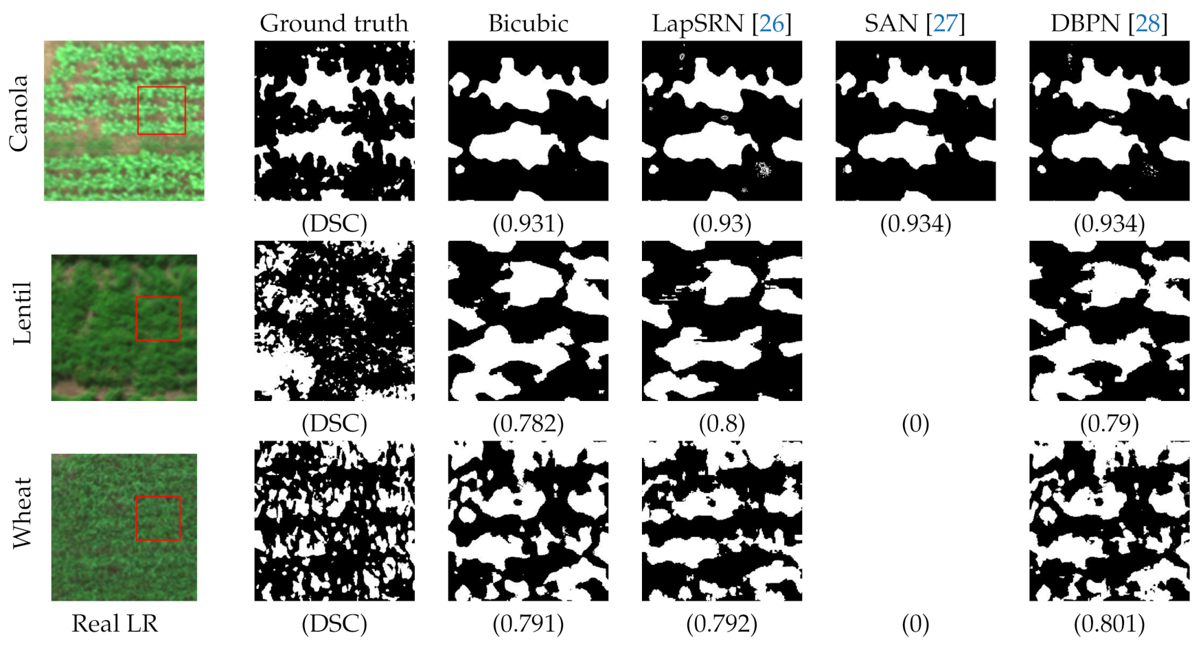
Figure 7 represents flower segmentation on the canola dataset employing the three different experiments.
Figure 8,
Figure 9 and
Figure 10 demonstrate vegetation segmentation on the canola, lentil and wheat datasets respectively, for the synthetic-synthetic, synthetic-real, and real-real experiments.
5. Discussion
In this study, we applied super resolution methods to aerial crop images to evaluate how well these methods work for image-based plant phenotyping. We have flown a UAV with two sensors to capture low and high resolution images of a field simultaneously, which enables us to train super resolution models with real-world images. Once trained, these super resolution models would allow a researcher, breeder or grower to fly a low-cost and low-resolution UAV and then enhance the resolution of their images with our pretrained models. We conducted three different experiments, including the synthetic-synthetic, synthetic-real, and real-real for training and testing super resolution models to demonstrate the efficacy of employing a real-world dataset in aerial image super resolution.
The synthetic-synthetic super resolution models have achieved comparable results with bicubic interpolation over the canola dataset and underperformed in comparison with bicubic interpolation over the lentil and wheat datasets on PSNR and SSIM values. The positive results are likely because the synthetic LR images, even when downsampled from HR images, are fairly clear and plant features can be well identified. However, the performance of the synthetic-synthetic experiment cannot guarantee achieving the same performance when the models were tested with real-world low resolution images.
The super resolution models trained in the synthetic-real experiment were not able to generalize the feature mapping function learned from synthetic LR image to unseen real-world LR images. This is likely due to the limited or missing overlap between the feature spaces of the two datasets [
98]. Small features learned during training on the real-world HR datasets do not exist in the real-world LR test set, because of the GSD differences between the two sensors. Consequently, the super resolution models were prone to overestimating, instead of reconstructing those small features, visualized in
Figure 5. The models also failed to reconstruct higher spatial resolution images with smaller pixel sizes to segment flowering and vegetation more precisely, shown in
Figure 7 and
Figure 9. Therefore, using synthetic data (downsampled HR images) to train super resolution models may not be a practical technique for agricultural analysis.
The super resolution models trained in the real-real experiment have achieved promising results with the canola dataset on both standard and agricultural measures. The lentil and wheat datasets achieved comparable results with bicubic interpolation on PSNR and SSIM values. The three-crop dataset has demonstrated close quantitative PSNR and SSIM values to the canola dataset, as shown in
Table 3 and
Table 4, meaning the distribution of the three-crop dataset is skewed towards the canola dataset.
The real-real experiment outperformed the synthetic-real experiment in every condition tested, therefore we conclude that creating a paired dataset of real-world low and high resolution images is essential for super resolution in agricultural analysis. The reconstructed images over the real-real experiment seem to be sufficiently reliable for the agricultural analysis tested. Plants like wheat which present visibly small phenotypes require smaller pixel size to accurately measure plant density, especially early in the growing season. In our case, the UAV was flown at a higher altitude over the lentil and wheat trials to capture the entirety of the two trials in a relatively short period of time (
Section 3.1). Consequently, from a given focal length at a higher altitude, the ground object scales are smaller and require higher spatial resolution.
Figure 10 demonstrates the performance of the super resolution models on the real-real experiment, where the smaller pixel sizes, resulting in higher spatial resolution with smaller GSD, aid in more accurate vegetation segmentation in the canola and lentil datasets, but not for the wheat images. This means that the wheat dataset requires either to be captured with higher resolution sensor or the remote sensing device flies at lower altitude.
Smaller pixel sizes also aid in more accurate flower segmentation on the canola dataset in the real-real experiment, as shown in
Figure 7. We did not assess flower segmentation on the lentil and wheat dataset, because the flowers on those crops tend to be too small or occluded in aerial imagery, particularly for our lentil and wheat trials that were captured from a higher UAV altitude. The difference between the real LR and ground truth of the lentil and wheat images is visualized in
Figure 6.
The importance of pixel size is related to mixed-pixel effects, where a pixel may contain multiple information about different phenotypes of a plant and image background. In such cases, general thresholding techniques such as Otsu’s method [
96] calculate a measure of spread for pixels segmented into foreground or background classes. Larger mixed pixels are likely to increase the error rate of plant trait estimation because the plant’s phenotype may dissolve in the background or foreground, as shown in
Figure 9, where foreground features such as flowers blend into the green background of vegetation.
The differential performance of the selected models over three different trials and experiments indicates that no model that performs best in every condition, given our dataset. Each model selected has a unique architecture leading to data dependent differences in performance. For post-upsampling architectures including SAN [
27], all computational processing occurs in a low spatial resolution space which decreases the computational cost, but can result in reconstruction compromises, especially with large scaling factors. In progressive learning architectures such as LapSRN [
26], a difficult task is decomposed into several simple tasks, which reduces the learning difficulty for larger scaling factors. However, as progressive learning is a stacked model, it relies on limited LR features in each block, which can result in lower performance, especially for small scaling factors. Iterative up and downsampling networks represented by DBPN [
28] in this work, benefit from the recurrence of internal patches across scales in input images [
71]. DBPN [
28] focuses on generating a deeper feature map by alternating between the low and high spatial resolution spaces and computing the reconstruction error in each up and downsampling block. For example, DBPN [
28] has outperformed the other models in PSNR values across the canola, lentil and wheat datasets over the real-real experiment, but SAN [
99] achieved similar performance to DBPN [
28] in SSIM values and flower segmentation. In vegetation detection, DBPN [
28] marginally outperformed the other model. The vegetation segmentation value of wheat dataset employing DBPN [
28] over the real-real experiment shows
improvement compared to bicubic interpolation, while LapSRN [
26] achieved
improvement and SAN [
99] failed to reproduce HR images. Consequently, we can conclude that DBPN [
28] generally performs better across a range of images, but could be outperformed by a small margin under specific circumstances. Using iterative up and downsampling networks for agricultural drone super resolution tasks seems like the most promising approach, and should be the default choice, all other things being equal.
One limitation of our dataset is the imbalanced training set. There are almost triple the number of canola images compared to the total number of images in the lentil and wheat datasets. One solution could be collecting additional data from the field. However, collecting such data can be expensive. Data augmentation dealing with different random transformations of the images to increase the samples in a dataset and improve variances, is a well-known technique in deep learning. Although, we employed general augmentation techniques, such as data flipping, or rotating in our case, more sophisticated techniques, such as instance-based augmentation and fusion-based augmentation [
100] could prove beneficial. Oversampling that resamples less frequent data to balance their amount in comparison with dominant data is another technique with an imbalanced dataset. In [
101], a mathematical characterization of image representation was proposed to oversample data for image super resolution by learning the dynamic of information within the image.
There are other possible solutions, such as synthetic minority oversampling technique (SMOTE) [
102] or generative adversarial network (GAN) [
103] to address oversampling minority samples in training set prior to fitting a model. These techniques are common in image classification [
104], but they might be feasible for a minority of sub-samples, such as different crop growth stages or different genotypes. Of particular interest for future work is to explore oversampling techniques on our dataset to produce highly variant sub-samples in the training set.


