Abstract
Infrared observation is an all-weather, real-time, large-scale precipitation observation method with high spatio-temporal resolution. A high-precision deep learning algorithm of infrared precipitation estimation can provide powerful data support for precipitation nowcasting and other hydrological studies with high timeliness requirements. The “classification-estimation” two-stage framework is widely used for balancing the data distribution in precipitation estimation algorithms, but still has the error accumulation issue due to its simple series-wound combination mode. In this paper, we propose a multi-task collaboration framework (MTCF), i.e., a novel combination mode of the classification and estimation model, which alleviates the error accumulation and retains the ability to improve the data balance. Specifically, we design a novel positive information feedback loop composed of a consistency constraint mechanism, which largely improves the information abundance and the prediction accuracy of the classification branch, and a cross-branch interaction module (CBIM), which realizes the soft feature transformation between branches via the soft spatial attention mechanism. In addition, we also model and analyze the importance of the input infrared bands, which lay a foundation for further optimizing the input and improving the generalization of the model on other infrared data. Extensive experiments based on Himawari-8 demonstrate that compared with the baseline model, our MTCF obtains a significant improvement by 3.2%, 3.71%, 5.13%, 4.04% in F1-score when the precipitation intensity is 0.5, 2, 5, 10 mm/h, respectively. Moreover, it also has a satisfactory performance in identifying precipitation spatial distribution details and small-scale precipitation, and strong stability to the extreme-precipitation of typhoons.
1. Introduction
Precipitation is the main driving force of the hydrological cycle. Precipitation estimation is an important issue in meteorology, climate, and hydrology research [1]. Real-time and accurate precipitation estimation can not only provide data for precipitation nowcasting [2] but also provide the data support for extreme-precipitation monitoring [3,4], flood simulation [5], and other meteorological and hydrological studies [6,7].
Precipitation estimation mainly relies on three observation means, i.e., rain gauge, weather radar, and remote sensing. The rain gauge can directly measure precipitation, however, as a point measurement method, it is spatially discontinuous and sparse [8,9], which makes the application limited. Weather radar can provide continuous observations with high spatial and temporal resolution [10]. However, radar imagery only covers an area with a radius of about 1 degree. In large-scale scenes, the application value of the radar data greatly depends on the deployment density of the radar observation network [11]. Satellite observation can provide global precipitation estimation with high temporal and spatial resolution, and fill the data gaps in the ocean, mountains, and the areas without radar and rain gauge [12,13]. That means in some research, such as marine meteorology, the satellite is an irreplaceable observation mean of precipitation data.
Remote sensing precipitation observations can be mainly divided into three categories: infrared (IR), passive microwave (PMW), and active microwave [14]. Compared with the latter two categories, infrared data has the advantage of high spatio-temporal resolution. So far, infrared (IR) data have been widely used in authoritative precipitation products, such as the Climate Prediction Center morphing technique (CMORPH) [15], the Precipitation Estimation from Remotely Sensed Information using Artificial Neural Networks (PERSIANN) [16], the Tropical Rainfall Measuring Mission (TRMM) [17], and the Global Precipitation Measurement (GPM) [18]. However, the release of these high-quality precipitation products has a certain time delay. Thus, it is impossible to support extreme precipitation monitoring and nowcasting which require high timeliness. How to design a lightweight and high-precision precipitation estimation algorithm for remote sensing infrared imagery is always an important research topic.
The development of artificial intelligence provides the possibility to solve this problem. Various machine learning techniques, e.g., random forest (RF), support vector machine (SVM), and artificial neural network (ANN), have been adopted to model the relationship between infrared observations and the precipitation intensity [19,20,21,22]. PERSIANN [16] is a classic algorithm based on Artificial Neural Network (ANN) for constructing the relationship between precipitation and infrared observations, which is developed by the University of California, cooperated with the National Aeronautics and Space Administration (NASA) and the National Oceanic and Atmospheric Administration (NOAA). The PERSIANN family also includes two other precipitation estimation products, i.e., PERSIANN-CCS [23] and PERSIANN-CDR [24]. PERSIANN-CCS improves PERSIANN via the predefined cloud patch feature. PERSIANN-CDR utilizes the National Centers for Environmental Prediction (NCEP) precipitation product to replace the PMW imagery used for model training in PERSIANN [24].
Although traditional machine learning methods have shown potential in precipitation detection and monitoring, deep learning (DL) methods are more accurate in processing the big data [25]. Tao et al. [26] propose a algorithm based on stacked Stacked Denoising Autoencoders (SDAE) [27] named PERSIANN-SDAE. They think that PERSIANNs are based on manually defined features, which limits the ability of precipitation estimation, and PERSIANN-SDAE has the advantage of automatically extracting features from infrared cloud images, which leads to higher accuracy. Nevertheless, the inefficient structure of SDAE also limits its ability to effectively use neighborhood information to estimate precipitation. Therefore, Sadeghi et al. [28] proposed a precipitation estimation algorithm based on Convolutional Neural Network (CNN) [29] named PERSIANN-CNN. The research demonstrates that extracting spatial features from a data-driven perspective can obtain precipitation information more effectively.
In recent years, the two-stage framework has been widely used in the deep-learning study of precipitation estimation [30,31,32,33], which including a preliminary “rain/no-rain” binary classification and a non-zero precipitation estimation. The core of the two-stage framework is utilizing the results of the binary classification task as the masks to filter the no-rain data of the precipitation estimation task and alleviate the data imbalance problem. To a certain extent, utilizing the masked data to train the precipitation estimation model could reduce the bias of the model for no-rain data which accounts for a large proportion. It has been proved that the two-stage framework with deep learning methods has the ability to provide more accurate and reliable precipitation estimation products than the PERSIANN products.
However, as shown in Section 4.4.1, we experimentally found that the accuracy of the single classification model is lower than that of the precipitation estimation model. It is obviously contrary to the perception that the classification is simpler than the non-linear regression problem, i.e., the estimation. An intuitive reason is that there is a large gap between the captured information from the supervision signals of the classification network and the estimation network. The supervision signal of the estimation network is the abundant quantitative precipitation intensity information, while the classification network is only the qualitative information, i.e., “rain/no-rain”. Although the above-mentioned two-stage framework obtains better results than the single estimation model by using the classification predictions as the masks for the estimation model, such a simple series-wound mode leads to the error accumulation phenomenon from classification model to estimation model. For example, some rainy pixels may be filtered directly in the estimation model as it is classified as no-rain by mistake, and then these pixels can not be predicted correctly in the estimation model. When the accuracy of the classification model is not satisfactory, this phenomenon will be more serious.
If a novel combination mode of the classification and estimation model can be designed, in which the error accumulation phenomenon can be alleviated, meanwhile, the ability to improve the data balance can also be retained, the accuracy of the precipitation estimation can be further improved. To achieve this goal, we propose a Multi-Task Collaboration deep learning Framework (MTCF) for precipitation estimation. The framework achieves a cross-branch positive information feedback loop based on the “classification-estimation” dual-branch multi-tasking learning mechanism. Specifically, we propose a multi-task consistency constraint mechanism, in which the information captured by the estimation branch is propagated back to the classification branch through gradients to improve the information abundance of the classification branch. At the same time, we propose a cross-branch interaction module (CBIM). Through the soft spatial attention mechanism, CBIM realizes the soft transfer of features from the classification branch to the estimation branch. In addition to alleviating the dilemma of data imbalance, it also reduces the error accumulation caused by the simple series method of the hard masks. Through the combination of the above two points, we realize a positive information feedback loop from estimation to classification and back to estimation. Extensive experiments based on Himawari-8 data demonstrate that our multi-task collaboration framework, compared with the previous two-stage “classification-estimation” framework, can derive high spatio-temporal resolution precipitation products with higher accuracy. Moreover, we also analyze the correlation between infrared bands of different wavelengths of Himawari-8 under different precipitation intensities to lay a foundation for optimizing the input and improve the generalization capability of the model to other infrared remote sensing data.
Our contributions can be summarized as follows:
- We proposed a multi-task collaboration framework named MTCF, i.e., a novel combination mode of the classification and estimation model, which alleviates the error accumulation and retains the ability to improve the data balance;
- We propose a multi-task consistency constraint mechanism. Through this mechanism, the information abundance and the prediction accuracy of the classification branch are largely improved;
- We propose a cross-branch interactive module, i.e., CBIM, which realizes the soft feature transformation between branches via the soft spatial attention mechanism. The consistency constraint mechanism and CBIM together make up a positive information feedback loop to produce more accurate estimation results;
- We model and analyze the correlation between infrared bands of different wavelengths of Himawari-8 under different precipitation intensities to improve the applicability of the model on other data.
2. Data
2.1. Himawari 8
Himawari-8 is a geostationary Earth orbit (GEO) satellite operated by the Japan Meteorological Agency (JMA). It performs a scan of East Asia and the Western Pacific every 10 min with a spatial resolution of 2 km. The Advanced Himawari Imager (AHI) on Himawari-8 is a 16-channel multispectral imager with 3 visible bands, 3 near-infrared bands, and 10 infrared bands as shown in Table 1.

Table 1.
The spectral parameters of Himawari-8.
Visible and near-infrared bands, which measure during the daytime, are usually used to retrieve cloud, aerosol, and vegetation characteristics or make real color pictures [34]. In order to reduce the influence of heterogeneous reflection of sunlight, in this paper, we choose to utilize all the infrared bands as the input of the model, i.e., bands 7–16. The infrared bands with different wavelengths can detect different information, such as cloud phase, cloud top temperature, cloud top height, and water vapor content at different heights, which could reflect the characteristics of precipitation indirectly [35].
2.2. GPM
The Global Precipitation Measurement (GPM) mission [36] is an international satellite precipitation observation network project initiated by the National Aeronautics and Space Administration (NASA) and Japan Aerospace Exploration Agency (JAXA). The core design of GPM is an extension of the last-generation Tropical Rainfall Measuring Mission (TRMM), which is mainly aimed at heavy to moderate rainfall in tropical and subtropical oceans. The main advancement of GPM is that it carries the first space-borne Ku/Ka-band Dual-frequency Precipitation Radar (DPR), which is more sensitive to light rain. The Integrated Multi-satellite Retrievals for GPM (IMERG) [37] algorithm combines multi-source information from the satellites operating around Earth, which can provide more accurate and reliable precipitation products for hydrology and other research.
In this paper, we take IMERG Final Run data as the reference for model training, which has a time resolution of 30 min and a spatial resolution of 0.1 degrees. The coverage of the IMERG Final Run data is shown in Figure 1.
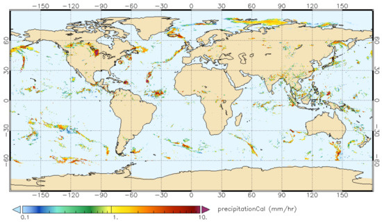
Figure 1.
An example of IMERG Final Run. It shows the precipitation intensity (mm/hr) from 07:00:00 to 07:29:59 in 20 September 2017.
2.3. Data Processing
In this paper, we study on the precipitation data from June to December in 2019, with 120° E to 168° E and 0° to 48° N as the research area, which contains relatively more high-intensity precipitation samples due to the frequent occurrence of typhoons. First, we preprocess the Himawari-8 and GPM data. As the spatial resolution of the Himawari-8 data is different from that of the GPM data, we resample the Himawari-8 data and unify the spatial resolution to 0.1 degrees via bilinear interpolation. After that, we perform the data matching on Himawari-8 data and GPM data. Since the time resolution of the former is higher than that of the latter, we refer to the timestamp of the GPM data to filter the Himawari-8 data and obtain a paired data set with a temporal resolution of 30 min. In order to make the model pay more attention to precipitation events, we further filter the data and exclude the samples whose precipitation area accounts for less than 1%. Finally, we totally get 5057 samples and adopt the strategy of random sampling by groups to divide them into the training data (3540 samples), validation data (506 samples), and test data (1011 samples) at a ratio of 7:1:2. Specifically, all the samples are sorted in time order and then divided into 100 groups evenly (43 groups with 50 samples each and 57 groups with 51 samples each ). From 100 groups, we randomly select 70 groups, 10 groups, and 20 groups as training data, validation data, and test data, respectively. The time distribution of the three datasets is shown in Figure S1 in the Supplementary Material.
In the following sections, we refer to the divided dataset as Infrared Precipitation Dataset (IRPD) and perform a series of experiments on the dataset.
2.4. Data Statistics
We calculate the distribution of precipitation intensity with different thresholds in IRPD as shown in Table 2. The Proportion refers to the ratio of the pixel number under a certain precipitation intensity to the total pixel number in IRPD. It can be seen that there is an obvious data imbalance problem in precipitation data. In addition, the relationship between the precipitation intensity and the precipitation level is also listed in Table 2.
Table 2.
The precipitation intensity statistics of IRPD.
3. Methods
In this section, we illustrate the proposed multi-task collaboration precipitation estimation framework (MTCF) in detail. First, we give an overview for the proposed MTCF for precipitation estimation. Second, we introduce the baseline network structure in our framework. Then, we elaborate on the proposed multi-branch network with the proposed consistency constraint mechanism. Finally, we illustrate the proposed cross-branch interaction module (CBIM) to improve the performance of precipitation estimation effectively.
3.1. Overview
In view of the disadvantages of the two-stage framework mentioned in Section 1, we propose a multi-task collaboration deep learning framework named MTCF for precipitation estimation. In MTCF, we design a cross-branch positive information feedback loop, which is composed of the multi-task consistency constraint mechanism and cross-branch interaction module. As shown in Figure 2, the whole framework consists of an encoder and two decoders, i.e., two parallel branches, which carry out the precipitation estimation and classification tasks, respectively.
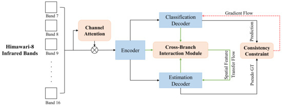
Figure 2.
The illustration of the proposed multi-task collaboration precipitation estimation framework (MTCF). MTCF contains an encoder and two parallel decoders (i.e., the precipitation classification and estimation branch). Here the red dotted line represents the gradient flow to the classification branch supervised by the estimation branch. The green lines depict the feature fusion process and spatial feature transfer process in the proposed cross-branch interaction module.
On the one hand, we introduce a consistency constraint mechanism into the loss function. To ensure the consistency of the predictions of the two parallel tasks, the mechanism calculates the consistency loss of the classification and estimation branch. In the process, we take the predictions of the estimation branch as the pseudo ground-truth. Thus, the information captured by the estimation branch can be propagated back to the classification branch via gradients to improve the information abundance and the classification accuracy of the classification branch. On the other hand, we propose a cross-branch interaction module (CBIM). It transmits the spatial features of the classification branch to the estimation branch and realizes the soft transfer and fusion of features between the two parallel branches. In addition to alleviating the dilemma of data imbalance, it also reduces the error accumulation (Error accumulation refers to the transfer of errors from the classification model to the estimation model in the process of using classification results to balance the data distribution for the estimation task) caused by the two-stage framework. The combination of the above two aspects forms a positive-going information propagation cycle of “estimation-classification-estimation”, and the experiments demonstrate that such design can achieve higher accuracy for precipitation estimation. Moreover, to explore the correlation between infrared bands of different wavelengths of Himawari-8, we introduce a channel attention module [38] before the encoder. By designing the corresponding experiments of different precipitation intensities, we obtain the change of the correlation of each infrared band under different precipitation intensities. During the experiments, we take the Himawari-8 data with 10 infrared bands as the input of the models and use the GPM data as the ground-truth for supervision.
3.2. Baseline Network
The precipitation estimation task aims at estimating per-pixel precipitation rate values, which is usually formulated as a segmentation-like problem [39,40]. In this paper, we take U-Net [41], which is a widely used model in image segmentation based on fully convolutional network (FCN) [42], as our baseline network. The baseline network consists of an encoder and a decoder. The encoder progressively reduces the spatial resolution and performs feature representation learning, while the decoder upsamples the feature maps and performs the pixel-level classification or regression. We give a detailed depiction of our baseline model as follows.
As shown in Figure 3, the encoder consists of the repeated application of double 3 × 3 convolutions, each followed by a rectified linear unit (ReLU) and a 2 × 2 max pooling operation with stride 2 for downsampling. The whole network has a downsampling ratio 16. The decoder contains three types of layers, including the repeated transposed convolution layer with stride 2 for upsampling, the ReLU layer, and the 3 × 3 convolution layer. Moreover, the feature maps in the encoder are directly concatenated with the ones of the same scale in the decoder to obtain accurate context information and achieve better prediction results. At the end of the network, a single convolution layer is added, which converts the channel number into 1, for the precipitation classification or estimation prediction.
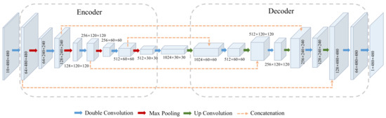
Figure 3.
The detailed architecture of our baseline network, i.e., U-Net.
3.3. Multi-Branch Network with Consistency Constraint
In the experiments of Section 4.4.1, we found that in the single classification and estimation task, the accuracy of the estimation task is significantly higher than that of the classification task under each precipitation intensity. We think the reason is that the information captured by the classification network is insufficient. Compared with the quantitative precipitation intensity information of the estimation task, the classification task can only obtain the qualitative information of “rain/no rain”, which leads to poor prediction results. In the multi-task precipitation estimation, the classification task plays a role of alleviating the data imbalance of precipitation estimation. Thus, it is extremely important to improve the accuracy of the classification task in order to reduce the negative impact of the error accumulation on the estimation task. To achieve this, one intuitive idea is that we can introduce the abundant quantitative precipitation information from the estimation branch to improve the information abundance for the classification model. Specifically, we design a consistency constraint mechanism between the two branches. By taking the predictions of the estimation branch as the pseudo ground-truth, the gap between the classification branch and the estimation branch is calculated and introduced into the loss function. In this way, the precipitation intensity information is further transmitted to the classification branch through gradient back-propagation to improve the accuracy of the classification branch.
As shown in Figure 4, the total loss function is composed of three parts: (1) the classification loss , (2) the estimation loss , and (3) the consistency loss . The classification branch aims at determining whether the precipitation rate at each pixel is larger than the threshold m (mm/h). We perform the binary cross-entropy loss computation for the classification branch. The estimation branch is designed to output the precipitation intensity (mm/h) concretely of each pixel. We use the mean squared error loss (MSE) and mean absolute error (MAE) loss for its supervision. In the consistency loss , let denote the predictions of the classification branch and represent the predictions of the estimation branch. Specifically, we transfer the estimation prediction to 0-1 mask as the pseudo ground-truth for the consistency loss. Its values are 1 if the prediction values in are larger than m and 0 otherwise. Then, we supervise by the mask to ensure the consistency of the two branches via the binary cross-entropy loss.
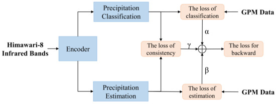
Figure 4.
The composition of total loss function, including the estimation loss, the classification loss, and the proposed consistency loss.
Thus, the total loss function is designed as follows:
where are the loss weights for balancing the three losses, and , , are the classification loss, estimation loss, and consistency loss, respectively.
3.4. Cross-Branch Interaction with Soft Attention
From Section 2.4, we observe that there exists obviously unbalanced distribution in precipitation data. Direct precipitation estimation on the unbalanced data will lead to the model being more inclined to no or light precipitation, which accounts for a larger proportion of the data. Thus, the prediction performance of the model for high-intensity precipitation will be unsatisfactory.
The two-stage solution is to serialize the classification and estimation task. Usually, it uses the predictions of the classification task to filter the precipitation data in the estimation task, which can adjust the distribution of data by removing the non-precipitation pixels. One obvious problem in this solution is that the classification task has a crucial, even decisive, influence on the estimation, and the error of the classification task will be directly reflected in the final estimation results.
In order to alleviate the error accumulation issue while using the predictions of the classification task to balance the data distribution in the estimation task, we proposed a cross-branch interaction attention mechanism. In this mechanism, we use the precipitation probability maps predicted by the classification branch as the soft spatial attention masks to carry out the multi-level feature transfer and fusion to the estimation branch. In this way, it can adjust the attention of the model to the data of different precipitation intensities and alleviate the problem of data imbalance.
As shown in Figure 5, the proposed cross-branch interaction module (CBIM) is inserted between the two parallel branches. The detailed process is described as follows and the detailed depiction of CBIM is shown in Figure 6. The detailed execution process in CBIM is described as follows.
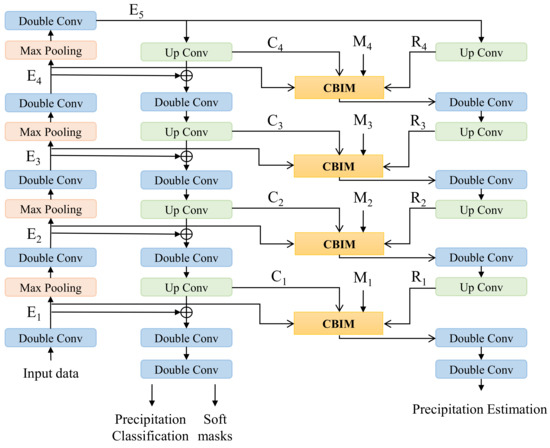
Figure 5.
The illustration of our MTCF. The proposed CBIM is inserted between the two parallel branches. Here E, R, and C denote the feature maps from the encoder, estimation branch, and classification branch, respectively. M denotes the output probability maps from the precipitation classification branch.
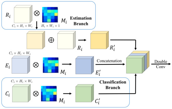
Figure 6.
The detailed architecture of the proposed cross-branch interaction module (CBIM). Here E, R, and C denote the feature maps from the encoder, estimation branch, and classification branch, respectively. M denotes the output probability maps from the precipitation classification branch. CBIM utilizes the precipitation probability maps predicted by the classification branch as soft masks to enhance the features of the corresponding positions in the estimation branch.
Let M denote the output probability maps from the precipitation classification branch. First, based on M, we generate four attention maps as shown in Figure 5, i.e., , , , , with different scales via bilinear interpolation, where and . Next, we use these resized attention maps, , to extract the region-aware estimation features. As shown in Figure 6, given the i-th stage feature maps in the precipitation estimation branch, the enhanced feature maps is calculated as follows:
where * indicates the element-wise multiplication operation. Then, we introduce the features from the classification branch, which can be denoted by , to the estimation branch. Specifically, we utilize the above attention mask to get the region-aware classification features, and the obtained features () are concatenated with the enhanced feature maps , the corresponding enhanced features () in the encoder. This process can be calculated as follows:
where denotes the concatenation operation and represents the corresponding feature maps in the encoder.
Finally, we use two sequential 1 × 1 convolution layers to refine the aggregated features and output the final features at stage i:
In this way, the features of the precipitation estimation branch are enhanced effectively via the proposed CBIM. So far, the proposed consistency constraint and CBIM have constituted the whole positive information feedback loop. The former realizes the information feedback from the estimation task to the classification task, which reduces the error of the classification branch. The latter realizes the information transfer from the classification task to the estimation task, which weakens the error accumulation of the classification branch. The model capacity can be largely and effectively improved through such a feedback loop and iteration, so as to realize the win-win situation of the multi-task model of the precipitation classification and estimation.
3.5. Implementation Details
In this section, we report the implementation details of our experiments. We conduct all the experiments based on Pytorch 1.1 [43] on a workstation with 2 GTX 1080 Ti GPU cards. During the training phase, the mini-batch size is set to 8 and the total training epoch is set to 150. The network parameters are optimized by Adam, with an initial learning rate 3 × 10, and a weight decay 1 × 10. The classification threshold m (mm/h) is set to 5.0 mm/h in our experiments. For the loss weights of the total loss function, are set to 1, 1, and 1, respectively. The principle of setting these loss weights is to make the three losses in the same order of magnitude, so as to ensure stable optimization in the multi-task learning.
4. Results
4.1. Evaluation Metrics
4.1.1. Precipitation Classification
As a pixel-level binary classification problem, each pixel in precipitation classification has
where m denotes the threshold of the classification branch, denotes the prediction results of the classification model, denotes the ground truth.
With comparing the prediction (P) and ground truth (T) values, there are four situations as shown in Table 3.
Table 3.
Criterion Table for Prediction Metrics.
The first situation is (True Positive, TP), which means the Prediction “Hits” the fact and give the true alarm. The second situation is (False Positive, FP), which means the Prediction gives “False Alarm”. The third situation is (False Negative, FN), which means the Prediction “Miss” the fact about precipitation level. The last situation is (True Negative, TN), which should be “Ignored”. With the above four situations, we can calculate some indexes.
The precision (Equation (7)) and recall (Equation (8)) are two evaluation indexes commonly used in binary classification.
It can be seen that precision is used to measure whether there is a misjudgment in the prediction, and it directly reflects the ability of the model to distinguish negative samples. The recall is used to measure whether there is any omission in the prediction and it reflects the ability to identify positive samples. A superior model should be able to balance the precision and recall at the same time. The F1-score (Equation (9)) is designed to consider both at the same time, which can indicate how effective the model is.
In our experiments, we use the precision, recall, and F1-score as the evaluation metrics for the classification task.
4.1.2. Precipitation Estimation
In order to evaluate the performance of the estimation model under different precipitation intensities and compare it with the classification model more intuitively, we convert the precipitation estimation into a pseudo-binary classification problem. Specially, we define a set of thresholds, M, for precipitation intensity. For , the precipitation estimation result and the ground-truth can be converted into the binary grids according to the Equation (6). For each precipitation intensity, the precipitation estimation also has four situations as shown in Table 3. The performance of the estimation model under a certain precipitation intensity threshold m can also be measured by the three evaluation metrics, i.e., , and , as the same as classification.
In addition, we also use standard quantitative scores, such as root mean squared error (RMSE), Pearson’s correlation coefficient, and ratio bias to evaluate the precipitation estimation results.
4.2. Quantitative Results
In this section, we show the quantitative results of the models on IRPD dataset. In order to evaluate the performance of the models under different precipitation intensities, we select a set of thresholds (i.e., 0.5 mm/h, 2 mm/h, 5 mm/h, 10 mm/h) based on the statistical results of the precipitation data distribution (Table 2), and calculate the evaluation metrics corresponding to each threshold, respectively. To evaluate the effectiveness of each proposed module in our framework, we show how performance gets improved by adding each component (i.e., the channel-attention module inserted before the encoder, the consistency constraint in Section 3.3 and the cross-branch interaction with soft attention (CBIM) in Section 3.4) step-by-step into our final model. Meanwhile, we compare our framework with PERSIANN-CNN [28] and the two-stage framework [30] to verify the effectiveness of our framework. The detailed results on the IRPD validation set are shown in Table 4.
Table 4.
The Precision, Recall, and F1-score of different models on the IRPD validation dataset. CA stands for the Channel Attention module which is inserted before the encoder, and CC stands for the Consistency Constraint of multi-branch. CBIM represents the proposed cross-branch interaction module with soft attention. The best result of each evaluation metric under different precipitation intensity is marked by bold face and the second best result is marked by underlining.
Compared with PERSIANN-CNN [28], U-Net [41], as our baseline, significantly improves the overall performance of the model. To be specific, U-Net surpasses PERSIANN-CNN by 3%–5% improvement in precision, and a large margin in recall (about 4% improvement at 0.5–2 mm/h, 9%–14% improvement at other precipitation intensities). The F1 score is also largely improved by 7%–12%. When the channel attention layer is added, there is a slight but relatively insignificant improvement in model performance. All the three evaluation measures (i.e., precision, recall, and F1) are improved by about 0.5%.
After adopting the multi-branch architecture and adding the proposed consistency constraint, i.e., U-Net+CA+CC, the overall performance is further improved, and the result of the model is the second-best among all the models. At the same time, it can be seen that the model at this time is similar to the two-stage model [30] in the case of low-intensity precipitation, but in the case of high-intensity precipitation, the F1 of U-Net+CA+CC is generally 2%–3% higher than that of the two-stage model. The result of the final model, i.e., MTCF, is the best among all the models, and significantly outperforms the two-stage framework [30] in all the evaluation metrics. Compared with the baseline model U-Net, MTCF has a comprehensive and significant improvement by 1.14%, 1.87%, 2.52%, 4.99% (m = 0.5, 2, 5, 10 mm/h) in precision, 5.05%, 5.19%, 6.96%, 3.38% (m = 0.5, 2, 5, 10 mm/h) in recall, and 3.2%, 3.71%, 5.13%, 4.04% (m = 0.5, 2, 5, 10 mm/h) in F1-score, respectively.
In order to verify the generalization ability of our model, we conduct the experiments of precipitation estimation on the test set of IRPD. In order to quantitatively and intuitively evaluate the performance of the model under different precipitation intensities, we defined a threshold set of precipitation intensity from 0.5 to 10 with an interval of 0.5. Based on this set, we plotted the precision, recall, and F1 values of the model with the change of precipitation intensity, which is shown in Figure 7.
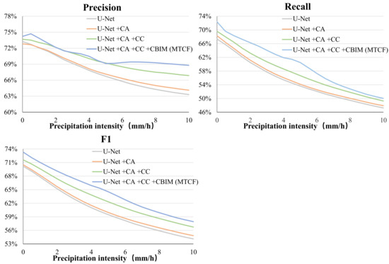
Figure 7.
The precision, recall, and F1 values of the model with the change of precipitation intensity.
As shown in Figure 7, the performance of the model on the test set is similar to that on the validation set. Among the three evaluation metrics, except for the final model, the performance increase in the other three models is basically stable or grows slowly with the change of precipitation intensity. It can be seen that U-Net+CA+CC significantly improves the baseline U-Net under all precipitation intensities, and our MTCF has a performance gain on the basis of U-Net+CA +CC. An interesting observation is that compared with U-Net+CA +CC, the F1 improvement of MTCF is generally uniform under different precipitation intensities. The improvement of precision in the case of precipitation intensity greater than 5.0 mm/h is far greater than that in the case of precipitation intensity less than 5.0 mm/h, and the improvement of recall in the case of precipitation intensity greater than 5.0 is far less than that in the case of precipitation intensity less than 5.0. Obviously, the reason is that the classification threshold in the classification branch is set to 5.0 mm/h. The CBIM enables the spatial features of the classification task to affect the precipitation estimation task through soft attention across branches. Thus, we conduct the ablation study on the threshold selection for the precipitation classification branch in Section 4.4.2 to select the most appropriate threshold.
In addition, we calculate the standard quantitative scores (i.e., Correlation, RMSE and ratio bias) between PERSIANN-CCS, PERSIANN-CNN, two-stage method and our models. The results are shown in Table 5. The improvement trend of the models is generally consistent with the Table 4, which can be seen from the changes of the RMSE and correlation. The decrease in the RMSE and the increase in the correlation indicate that the addition of the CA, CC, and CBIM modules improves the model performance steadily. The bias ratio represents the overall deviation degree of the estimation. The bias ratio of U-Net+Ca+CC+CBIM is the closest to 1, and it is also the only one greater than 1, while other models all underestimate precipitation. The bias ratio of the two-stage is the second closest to 1. This is due to the data balance ability of the two-stage model, which can reduce the bias of the model on “no-rain" and alleviate the underestimation to a certain extent. However, the two-stage framework does not consider the error accumulation, which leads to an inferior performance to U-NET+CA+CC+CBIM.
Table 5.
The RMSE, Correlation, and ratio bias of different models compared with GPM and PERSIANN-CCS. The best result of each score is marked by bold face and the second result is marked by underlining.
4.3. Visualization Results
In order to verify the generalization ability of our MTCF and show the prediction results qualitatively, we also perform precipitation estimation on the test set of IRPD and visualize some test examples to compare the performance of models more intuitively. The visualization results are shown in Figure 8.
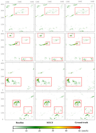
Figure 8.
The visualization comparison of our MTCF with the baseline U-Net. There are four examples in the figure, one for each row. The four precipitation events from top to bottom occurred at 13:30 on 2 June 2019, 8:30 on 19 June 2019, 2:00 on 16 July 2019, and 17:00 on 10 October 2019, respectively. The last example contains the precipitation of Typhoon Hagibis in 2019.
We select four examples to compare the baseline U-Net, MTCF, and the ground-truth. From the box selection area in the first row, it is clear that the estimation results of our MTCF contain more details about spatial distribution. Compared with the baseline model, MTCF can detect more small regional precipitation events, and its estimation results are closer to those of GPM precipitation products. From the box selection area in the second row, it can be seen that MTCF also significantly performs better than the baseline in the estimation of high-intensity precipitation, which is reflected in its ability to more accurately identify the spatial characteristics of high-intensity precipitation areas. However, through the box selection in the upper left corner, it is also found that although the spatial characteristics of MTCF are basically consistent with the ground-truth and better than the baseline, there is still a certain degree of underestimation for small-scale high-intensity precipitation. The example in the third line also proves the excellent ability of MTCF in capturing the spatial distribution characteristics of precipitation and detecting precipitation events in small regions. It also shows that there are still some deficiencies in the prediction of high-intensity precipitation. The fourth example includes the precipitation of Typhoon Hagibis in 2019. The visualization results show that the performance of our MTCF remains stable when dealing with extreme weather conditions, such as typhoons. Compared with the baseline, both the detection of high-intensity precipitation and the identification of detailed characteristics of the spatial distribution of precipitation have a significant improvement.
4.4. Ablation Study
4.4.1. The Effectiveness of Multi-Task Collaboration
To verify the effectiveness of our multi-task collaboration framework, in this section, we conduct the following experiments. We use the rainfall intensity of 5.0 mm/h as the threshold for precipitation classification, and compare the results of the single U-Net for the classification and estimation task, respectively. Meanwhile, we compare them with the prediction results of the proposed MTCF and the corresponding results are shown in Table 6.
Table 6.
The prediction results of the single U-net for classification and estimation task and the prediction results of our MTCF.
It can be seen that the accuracy of the single U-Net in the classification task is much lower than that of estimation, that is, with the difference of 14.8% in Precision and 7.15% in F1. We consider that the reason is that the classification model can only obtain the quantitative information of “0–1”, while the estimation model can obtain the specific precipitation intensity information. This difference makes the cognitive ability of the classification model significantly weaker than that of the estimation model. Therefore, in this kind of background, the two-stage framework uses the classification results as the masks to filter the precipitation data for the estimation task, in which the error of the classification model will directly have a negative impact on the estimation model results. Specifically, the FN situation (as shown in Table 3) of the classification model makes some pixels, which are actually with precipitation, directly filtered. The FP situation of the classification model makes some no precipitation data not filtered which weakens the data balance effect on the estimation model.
As shown in Table 6, after utilizing the proposed multi-task collaboration framework, the accuracy of the classification task is improved to the same level as the estimation model. Compared with the single U-net for classification, the accuracy of classification in the MTCF is greatly improved. Meanwhile, the accuracy of the estimation task in the MTCF is also significantly higher than that of the single U-net for estimation, with 2.52% gains in prediction, 5.96% gains in recall, and 5.13% gains in F1-score. The reason is that the difficulty of the classification task is lower than that of the estimation task. When the two tasks obtain the same amount of information, the accuracy of the classification results will be higher than that of the estimation. At this time, transferring the classification results or features to the estimation model can help adjust the data distribution of the estimation model, reduce the difficulty of the estimation task to a certain extent, and improve the prediction accuracy of the estimation task.
Therefore, the multi-task collaboration framework based on the positive information feedback loop is essentially a win-win model. It constructs an effective information exchange loop between the parallel classification and estimation branches. On the one hand, the rich information of the estimation model is transferred to the classification model, and on the other hand, the results and features of the classification model are used to assist in reducing the cognitive difficulty of the estimation model. In the training phase, the information has gone through a cycle of iterations, and finally achieved a consistent improvement in the accuracy of the classification task and the estimation model.
4.4.2. The Impact of the Classification Threshold
It can be seen from the previous discussion that in our MTCF, the classification results and features of the classification branch have a great influence on the estimation task. The threshold selection of the classification task will affect the performance of the estimation model under different precipitation intensities. In this section, we explore the influence of different threshold selections of the classification task on the estimation task. Specifically, we select 0.01 mm/h, 0.5 mm/h, 2.0 mm/h, 5 mm/h and 10 mm/h as the threshold values of the classification branches. The precision, recall, and F1 of the estimation branch under different rainfall intensities are shown in Table 7. Each row represents the performance of the estimation branch under different thresholds at a specific rainfall intensity We bold the best result of each line and underline the second-best result.
Table 7.
The precipitation results under different classification threshold values. Each row represents the performance of the estimation branch under different thresholds at a specific rainfall intensity.
As shown in Table 7, when the classification threshold is 5.0 mm/h, the F1 of the estimation model is the highest under the rainfall intensity of 5 mm/h and 10 mm/h, and it is the second-best under the rainfall intensity of 0.5 mm/h and 2mm/h. F1 score, as a comprehensive evaluation index considering precision and recall, can represent the overall performance of the model. Therefore, when the classification threshold is 5.0 mm/h, the overall performance of the estimation model under each precipitation intensity achieves the best performance. When 0.5 mm/h, 2 mm/h, or 10 mm/h is taken as the classification threshold, the model only performs well under the corresponding or adjacent precipitation intensity, but it does not perform well under other precipitation intensities. When the classification threshold is set to 0.01 mm/h, the precision is outstanding, while the low recall leads to an unsatisfactory performance (i.e., F1) of the model.
From the perspective of the application significance, precipitation estimation, as the data foundation of the flood control and disaster mitigation, should pay more attention to the high-intensity precipitation. Therefore, considering the model performance and the application significance, we finally choose 5.0 mm/h as the threshold value of the classification task in our proposed multi-task collaboration framework.
4.5. The Analysis of Band Correlation
How to apply the model to other GEO satellites with different frequency band designs, using as few channels as possible, requires further understanding of the importance of different frequency bands in the model [33]. We introduce the channel attention module, which is presented in Squeeze-and-Excitation Networks (SE-Net) [44], into our framework. The channel attention module can model the correlation of feature channels. By introducing the module, the attention of the model to different bands can be adjusted and the accuracy of the model can also be slightly improved. More importantly, the importance of each input band in the model can be captured.
To explore the importance of each infrared band in Himawari-8 for precipitation with different intensities, we perform a series of comparative experiments. Specifically, we insert the channel attention module before the encoder of the classification and estimation model of precipitation intensity 0.5, 5.0, and 10, respectively, and output the channel weights of input bands obtained in each model. The corresponding results are shown in Figure 9. As the weight represents the relative importance of each band in the model, it is difficult to make a direct comparison between different models. We sort the band weight values of each model to facilitate the comparison between models. The sorted results are shown in Figure 10.
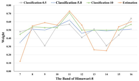
Figure 9.
The channel weights of input bands obtained in the models with different classification threshold values.
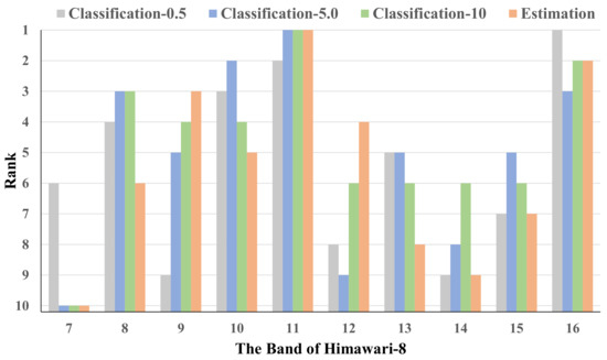
Figure 10.
The sorted band weights of the models with different classification threshold values.
In general, the band-11 has the highest weight among all models. As shown in Table 1, band-11(8.59 μm) can detect the cloud phase information, which has been applied in a series of studies such as PRESIANN-CCS [23]. In addition to the band-11, the band-16 also has a relatively high weight. The band-16 (13.28 μm) can reflect the cloud top height information. Some studies [45,46,47,48] show that there is a strong correlation between the cloud top height information and the precipitation intensity. Moreover, the band-8 (6.24 μm, band-9 (6.94 μm), and band-10 (7.35 μm) can detect the upper troposphere water vapor density, the middle to upper troposphere water vapor density, and the middle troposphere water vapor density, respectively, which is significantly correlated with precipitation and also verified in Figure 9.
In the classification model with thresholds of 0.5 and 5, the weight of the band-10 is higher than that of the band-8. In the classification model with the threshold of 10, the weight of band-10 is lower than that of band-8. In the precipitation estimation model, which needs to consider higher precipitation intensity, the weight of the band-10 is also higher than that of the band-8. At the same time, with the increase in precipitation intensity that the model focuses on, the importance of the band-9 also increases. This indicates that water vapor density in the middle troposphere has a high correlation with weak precipitation, while water vapor density in the middle to the upper troposphere and upper troposphere has a higher correlation with high-intensity precipitation.
5. Discussion
Considering the evaluation results of our model, the visualization results of our model, and the related experimental analysis mentioned above, we have the following observations and discussions:
- The performance of the single U-Net classification model is worse than that of the single U-Net estimation model. We suspect that this is caused by the fact that the information abundance obtained by the classification model is much lower than that obtained by the estimation model, which makes the cognitive ability of the classification model significantly weaker than that obtained by the estimation model. The two-stage framework, in which the above two models are connected in series through masks to alleviate the data imbalance problem, will result in the accumulation of classification errors and limit the accuracy improvement of the model to a certain extent. This is also the main reason why the accuracy of the two-stage framework is lower than our multi-task collaboration framework.
- The consistency constraint and the CBIM can effectively improve the accuracy of the model under different precipitation intensities. Figure 8 shows that MTCF can predict the precipitation spatial distribution and small-scale precipitation in more detail, and also has a superior performance in typhoon precipitation prediction. The reason is that the consistency constraint enhances the information abundance of the classification model through the gradient back-propagation and improves the cognitive ability of the classification model. The CBIM changes the spatial attention of the estimation model to the precipitation data by transmitting the classification predictions and spatial features, so as to enhance the estimation capacity of the model for high-intensity precipitation. The combination of the above two forms a positive information feedback loop of “estimation-classification-estimation”, which makes the accuracy of both the classification model and estimation model significantly improved.
- By introducing the channel attention module, the model has a small and relatively insignificant performance improvement. However, more importantly, we can observe the importance of the input bands in the model by this. From the comparison, we observe that the band-11 (8.59 μm) and the band-16 (13.28 μm) are related to the precipitation intensity, and these two bands can monitor cloud phase and cloud top height, respectively, which has been verified in some works [23,45,46,47,48]. In addition, the changes of the weights of band-8, band-9, and band-10 under different precipitation intensities indicate that the correlation between the low-intensity precipitation and water vapor density in the middle troposphere is great, meanwhile, the high-intensity precipitation has a great correlation with water vapor density in the higher troposphere.
- Although the multi-task collaboration framework can effectively improve the accuracy under each precipitation intensity, the estimation accuracy of high-intensity precipitation, which has attracted great attention in production and life, flood control and disaster prevention, and other applications, is still not ideal. We suspect that the complex patterns of high-intensity precipitation and the scarcity of samples increase the difficulty of the model training. In addition, the errors in GPM are also a potential cause.
In the future, we will (1) further construct a multi-task collaboration framework with a multi-classification architecture or multi-binary architecture to improve the estimation ability of the model for high-intensity precipitation; (2) explore the input bands and the combination between bands, model the importance of bands in precipitation estimation and improve the input of the model based on this.
6. Conclusions
In this paper, we have proposed a multi-task collaboration deep learning framework named MTCF for remote sensing infrared precipitation estimation. In this framework, we have developed a novel parallel cooperative combination mode of the classification and estimation model, which is realized by the consistency constraint mechanism and a cross-branch interaction module (CBIM) with soft attention. Compared to the simple series-wound combination mode of the previous two-stage framework, our framework has alleviated the error accumulation problem in multi-tasking and retained the ability to improve the data balance. Extensive experiments based on the Himawari-8 and GPM dataset have demonstrated the effectiveness of our framework against the two-stage framework and PERSIANN-CNN methods.
From the perspective of the application, our framework is lightweight, real-time, and high-precision with a strong identification ability of the precipitation spatial distribution details and a generalization ability of extreme weather conditions. It can provide strong data support for short-term precipitation prediction, extreme weather monitoring, flood control, and disaster prevention. In addition, the importance of the input infrared bands obtained in our work will lay a foundation for optimizing the input of the precipitation estimation and improving the generalization capability of our model to other infrared remote sensing data in the future. We hope that the novel multi-tasking collaborative framework proposed by us will serve as a solid framework and benefit other research in precipitation estimation in the future.
Supplementary Materials
The following are available online at https://www.mdpi.com/article/10.3390/rs13122310/s1.
Author Contributions
Conceptualization, X.Y.; Methodology, X.Y. and P.S.; Funding acquisition, F.Z., Z.D. and R.L.; Project administration, R.L.; Writing—original draft preparation, X.Y. and P.S.; Writing—review and editing, F.Z. All authors have read and agreed to the published version of the manuscript.
Funding
This research was funded by the National Key R&D Program of China (2018YFB0505000), National Natural Science Foundation of China (41671391, 41922043, 41871287).
Data Availability Statement
The following datasets are used in this study:
- Himawari-8: Data can be obtained from JAXA Himawari Monitor system and are available at ftp.ptree.java.jp accessed on 15 October 2020 after applying for an account.
- GPM IMERG data: Data can be obtained from NASA EarthData webpage and are available at https://disc.gsfc.nasa.gov/datasets/GPM_3IMERGHH_06/summary?keywords=GPM accessed on 3 December 2019.
Acknowledgments
We would like to thank Japan Aerospace Exploration Agency (JAXA) for providing Himawari-8 data and National Aeronautics and Space Administration (NASA) PPS for providing GPM IMERG data.
Conflicts of Interest
The authors declare no conflict of interest.
References
- Trenberth, K.E.; Dai, A.; Rasmussen, R.M.; Parsons, D.B. The changing character of precipitation. Bull. Am. Meteorol. Soc. 2003, 84, 1205–1218. [Google Scholar] [CrossRef]
- Akbari Asanjan, A.; Yang, T.; Gao, X.; Hsu, K.; Sorooshian, S. Short-range quantitative precipitation forecasting using Deep Learning approaches. In Proceedings of the AGU Fall Meeting Abstracts, New Orleans, LA, USA, 11–15 December 2017; Volume 2017, p. H32B-02. [Google Scholar]
- Nguyen, P.; Sellars, S.; Thorstensen, A.; Tao, Y.; Ashouri, H.; Braithwaite, D.; Hsu, K.; Sorooshian, S. Satellites track precipitation of super typhoon Haiyan. Eos Trans. Am. Geophys. Union 2014, 95, 133–135. [Google Scholar] [CrossRef]
- Scofield, R.A.; Kuligowski, R.J. Status and outlook of operational satellite precipitation algorithms for extreme-precipitation events. Weather Forecast. 2003, 18, 1037–1051. [Google Scholar] [CrossRef]
- Arnaud, P.; Bouvier, C.; Cisneros, L.; Dominguez, R. Influence of rainfall spatial variability on flood prediction. J. Hydrol. 2002, 260, 216–230. [Google Scholar] [CrossRef]
- Foresti, L.; Reyniers, M.; Seed, A.; Delobbe, L. Development and verification of a real-time stochastic precipitation nowcasting system for urban hydrology in Belgium. Hydrol. Earth Syst. Sci. 2016, 20, 505. [Google Scholar] [CrossRef]
- Beck, H.E.; Vergopolan, N.; Pan, M.; Levizzani, V.; Van Dijk, A.I.; Weedon, G.P.; Brocca, L.; Pappenberger, F.; Huffman, G.J.; Wood, E.F. Global-scale evaluation of 22 precipitation datasets using gauge observations and hydrological modeling. Hydrol. Earth Syst. Sci. 2017, 21, 6201–6217. [Google Scholar] [CrossRef]
- Gehne, M.; Hamill, T.M.; Kiladis, G.N.; Trenberth, K.E. Comparison of global precipitation estimates across a range of temporal and spatial scales. J. Clim. 2016, 29, 7773–7795. [Google Scholar] [CrossRef]
- Folino, G.; Guarascio, M.; Chiaravalloti, F.; Gabriele, S. A Deep Learning based architecture for rainfall estimation integrating heterogeneous data sources. In Proceedings of the 2019 International Joint Conference on Neural Networks (IJCNN), Budapest, Hungary, 14–19 July 2019; pp. 1–8. [Google Scholar]
- Habib, E.; Haile, A.T.; Tian, Y.; Joyce, R.J. Evaluation of the high-resolution CMORPH satellite rainfall product using dense rain gauge observations and radar-based estimates. J. Hydrometeorol. 2012, 13, 1784–1798. [Google Scholar] [CrossRef]
- Westrick, K.J.; Mass, C.F.; Colle, B.A. The limitations of the WSR-88D radar network for quantitative precipitation measurement over the coastal western United States. Bull. Am. Meteorol. Soc. 1999, 80, 2289–2298. [Google Scholar] [CrossRef]
- Chang, N.B.; Hong, Y. Multiscale Hydrologic Remote Sensing: Perspectives and Applications; CRC Press: Boca Raton, FL, USA, 2012. [Google Scholar]
- Ajami, N.K.; Hornberger, G.M.; Sunding, D.L. Sustainable water resource management under hydrological uncertainty. Water Resour. Res. 2008, 44. [Google Scholar] [CrossRef]
- Hong, Y.; Tang, G.; Ma, Y.; Huang, Q.; Han, Z.; Zeng, Z.; Yang, Y.; Wang, C.; Guo, X. Remote Sensing Precipitation: Sensors, Retrievals, Validations, and Applications; Observation and Measurement; Li, X., Vereecken, H., Eds.; Springer: Berlin/Heidelberg, Germany, 2019; pp. 1–23. [Google Scholar]
- Joyce, R.J.; Janowiak, J.E.; Arkin, P.A.; Xie, P. CMORPH: A method that produces global precipitation estimates from passive microwave and infrared data at high spatial and temporal resolution. J. Hydrometeorol. 2004, 5, 487–503. [Google Scholar] [CrossRef]
- Hsu, K.l.; Gao, X.; Sorooshian, S.; Gupta, H.V. Precipitation estimation from remotely sensed information using artificial neural networks. J. Appl. Meteorol. 1997, 36, 1176–1190. [Google Scholar] [CrossRef]
- Huffman, G.J.; Bolvin, D.T.; Nelkin, E.J.; Wolff, D.B.; Adler, R.F.; Gu, G.; Hong, Y.; Bowman, K.P.; Stocker, E.F. The TRMM Multisatellite Precipitation Analysis (TMPA): Quasi-global, multiyear, combined-sensor precipitation estimates at fine scales. J. Hydrometeorol. 2007, 8, 38–55. [Google Scholar] [CrossRef]
- Huffman, G.J.; Bolvin, D.T.; Braithwaite, D.; Hsu, K.; Joyce, R.; Xie, P.; Yoo, S.H. NASA global precipitation measurement (GPM) integrated multi-satellite retrievals for GPM (IMERG). Algorithm Theor. Basis Doc. (ATBD) Version 2015, 4, 26. [Google Scholar]
- Bellerby, T.; Todd, M.; Kniveton, D.; Kidd, C. Rainfall estimation from a combination of TRMM precipitation radar and GOES multispectral satellite imagery through the use of an artificial neural network. J. Appl. Meteorol. 2000, 39, 2115–2128. [Google Scholar] [CrossRef]
- Ba, M.B.; Gruber, A. GOES multispectral rainfall algorithm (GMSRA). J. Appl. Meteorol. 2001, 40, 1500–1514. [Google Scholar] [CrossRef]
- Behrangi, A.; Hsu, K.L.; Imam, B.; Sorooshian, S.; Huffman, G.J.; Kuligowski, R.J. PERSIANN-MSA: A precipitation estimation method from satellite-based multispectral analysis. J. Hydrometeorol. 2009, 10, 1414–1429. [Google Scholar] [CrossRef]
- Ramirez, S.; Lizarazo, I. Detecting and tracking mesoscale precipitating objects using machine learning algorithms. Int. J. Remote Sens. 2017, 38, 5045–5068. [Google Scholar] [CrossRef]
- Sorooshian, S.; Hsu, K.L.; Gao, X.; Gupta, H.V.; Imam, B.; Braithwaite, D. Evaluation of PERSIANN system satellite-based estimates of tropical rainfall. Bull. Am. Meteorol. Soc. 2000, 81, 2035–2046. [Google Scholar] [CrossRef]
- Ashouri, H.; Hsu, K.L.; Sorooshian, S.; Braithwaite, D.K.; Knapp, K.R.; Cecil, L.D.; Nelson, B.R.; Prat, O.P. PERSIANN-CDR: Daily precipitation climate data record from multisatellite observations for hydrological and climate studies. Bull. Am. Meteorol. Soc. 2015, 96, 69–83. [Google Scholar] [CrossRef]
- LeCun, Y.; Bengio, Y.; Hinton, G. Deep learning. Nature 2015, 521, 436–444. [Google Scholar] [CrossRef]
- Tao, Y.; Gao, X.; Ihler, A.; Hsu, K.; Sorooshian, S. Deep neural networks for precipitation estimation from remotely sensed information. In Proceedings of the 2016 IEEE Congress on Evolutionary Computation (CEC), Vancouver, BC, Canada, 24–29 July 2016; pp. 1349–1355. [Google Scholar]
- Vincent, P.; Larochelle, H.; Lajoie, I.; Bengio, Y.; Manzagol, P.A.; Bottou, L. Stacked denoising autoencoders: Learning useful representations in a deep network with a local denoising criterion. J. Mach. Learn. Res. 2010, 11, 3371–3408. [Google Scholar]
- Sadeghi, M.; Asanjan, A.A.; Faridzad, M.; Nguyen, P.; Hsu, K.; Sorooshian, S.; Braithwaite, D. Persiann-cnn: Precipitation estimation from remotely sensed information using artificial neural networks—Convolutional neural networks. J. Hydrometeorol. 2019, 20, 2273–2289. [Google Scholar] [CrossRef]
- Albawi, S.; Mohammed, T.A.; Al-Zawi, S. Understanding of a convolutional neural network. In Proceedings of the 2017 International Conference on Engineering and Technology (ICET), Antalya, Turkey, 21–23 August 2017; pp. 1–6. [Google Scholar]
- Tao, Y.; Hsu, K.; Ihler, A.; Gao, X.; Sorooshian, S. A two-stage deep neural network framework for precipitation estimation from bispectral satellite information. J. Hydrometeorol. 2018, 19, 393–408. [Google Scholar] [CrossRef]
- Moraux, A.; Dewitte, S.; Cornelis, B.; Munteanu, A. Deep learning for precipitation estimation from satellite and rain gauges measurements. Remote Sens. 2019, 11, 2463. [Google Scholar] [CrossRef]
- Hayatbini, N.; Kong, B.; Hsu, K.L.; Nguyen, P.; Sorooshian, S.; Stephens, G.; Fowlkes, C.; Nemani, R.; Ganguly, S. Conditional Generative Adversarial Networks (cGANs) for Near Real-Time Precipitation Estimation from Multispectral GOES-16 Satellite Imageries—PERSIANN-cGAN. Remote Sens. 2019, 11, 2193. [Google Scholar] [CrossRef]
- Wang, C.; Xu, J.; Tang, G.; Yang, Y.; Hong, Y. Infrared precipitation estimation using convolutional neural network. IEEE Trans. Geosci. Remote Sens. 2020, 58, 8612–8625. [Google Scholar] [CrossRef]
- Miller, S.D.; Schmit, T.L.; Seaman, C.J.; Lindsey, D.T.; Gunshor, M.M.; Kohrs, R.A.; Sumida, Y.; Hillger, D. A sight for sore eyes: The return of true color to geostationary satellites. Bull. Am. Meteorol. Soc. 2016, 97, 1803–1816. [Google Scholar] [CrossRef]
- Thies, B.; Nauß, T.; Bendix, J. Discriminating raining from non-raining clouds at mid-latitudes using meteosat second generation daytime data. Atmos. Chem. Phys. 2008, 8, 2341–2349. [Google Scholar] [CrossRef]
- Hou, A.Y.; Kakar, R.K.; Neeck, S.; Azarbarzin, A.A.; Kummerow, C.D.; Kojima, M.; Oki, R.; Nakamura, K.; Iguchi, T. The Global Precipitation Measurement Mission. Bull. Am. Meteorol. Soc. 2013, 95, 701–722. [Google Scholar] [CrossRef]
- Huffman, G.; Bolvin, D.; Braithwaite, D.; Hsu, K.; Joyce, R.; Kidd, C.; Nelkin, E.; Sorooshian, S.; Tan, J.; Xie, P. Algorithm Theoretical Basis Document (ATBD) Version 4.5: NASA Global Precipitation Measurement (GPM) Integrated Multi-SatellitE Retrievals for GPM (IMERG); NASA: Greenbelt, MD, USA, 2015.
- Hu, J.; Shen, L.; Albanie, S.; Sun, G.; Wu, E. Squeeze-and-Excitation Networks. IEEE Trans. Pattern Anal. Mach. Intell. 2020, 42, 2011–2023. [Google Scholar] [CrossRef] [PubMed]
- Lebedev, V.; Ivashkin, V.; Rudenko, I.; Ganshin, A.; Molchanov, A.; Ovcharenko, S.; Grokhovetskiy, R.; Bushmarinov, I.; Solomentsev, D. Precipitation nowcasting with satellite imagery. In Proceedings of the 25th ACM SIGKDD International Conference on Knowledge Discovery & Data Mining, Anchorage, AK, USA, 4–8 August 2019; pp. 2680–2688. [Google Scholar]
- Lou, A.; Chandran, E.; Prabhat, M.; Biard, J.; Kunkel, K.; Wehner, M.F.; Kashinath, K. Deep Learning Semantic Segmentation for Climate Change Precipitation Analysis. In Proceedings of the AGU Fall Meeting Abstracts, San Francisco, CA, USA, 9–13 December 2019; Volume 2019, p. GC43D-1350. [Google Scholar]
- Ronneberger, O.; Fischer, P.; Brox, T. U-net: Convolutional networks for biomedical image segmentation. In Lecture Notes in Computer Science, Proceedings of the International Conference on Medical Image Computing and Computer-Assisted Intervention, Munich, Germany, 5–9 October 2015; Springer: Cham, Switzerland, 2015; pp. 234–241. [Google Scholar]
- Long, J.; Shelhamer, E.; Darrell, T. Fully convolutional networks for semantic segmentation. In Proceedings of the IEEE Conference on Computer Vision and Pattern Recognition, Boston, MA, USA, 8–12 June 2015; pp. 3431–3440. [Google Scholar]
- Paszke, A.; Gross, S.; Massa, F.; Lerer, A.; Bradbury, J.; Chanan, G.; Killeen, T.; Lin, Z.; Gimelshein, N.; Antiga, L.; et al. Pytorch: An imperative style, high-performance deep learning library. In Proceedings of the Advances in Neural Information Processing Systems, Vancouver, BC, Canada, 8–14 December 2019; pp. 8026–8037. [Google Scholar]
- Hu, J.; Shen, L.; Sun, G. Squeeze-and-excitation networks. In Proceedings of the IEEE conference on computer vision and pattern recognition, Salt Lake City, UT, USA, 18–22 June 2018; pp. 7132–7141. [Google Scholar]
- Arkin, P.A.; Meisner, B.N. The relationship between large-scale convective rainfall and cold cloud over the western hemisphere during 1982–1984. Mon. Weather Rev. 1987, 115, 51–74. [Google Scholar] [CrossRef]
- Adler, R.F.; Negri, A.J. A satellite infrared technique to estimate tropical convective and stratiform rainfall. J. Appl. Meteorol. 1988, 27, 30–51. [Google Scholar] [CrossRef]
- Cotton, W.R.; Anthes, R.A. Storm and Cloud Dynamics; Academic Press: Cambridge, MA, USA, 1992. [Google Scholar]
- Xu, L.; Sorooshian, S.; Gao, X.; Gupta, H.V. A cloud-patch technique for identification and removal of no-rain clouds from satellite infrared imagery. J. Appl. Meteorol. 1999, 38, 1170–1181. [Google Scholar] [CrossRef]


Publisher’s Note: MDPI stays neutral with regard to jurisdictional claims in published maps and institutional affiliations. |
© 2021 by the authors. Licensee MDPI, Basel, Switzerland. This article is an open access article distributed under the terms and conditions of the Creative Commons Attribution (CC BY) license (https://creativecommons.org/licenses/by/4.0/).