Full-Wave Modeling and Inversion of UWB Radar Data for Wave Propagation in Cylindrical Objects

Abstract

The nondestructive characterization of cylindrical objects is needed in many fields, such as medical diagnostics, tree trunk inspection, or concrete column testing. In this study, the radar equation of Lambot et al. is combined with cylindrical Green’s functions to fully model and invert ultra-wideband (UWB) ground-penetrating radar (GPR) data and retrieve the properties of cylindrical objects. Inversion is carried out using a lookup table (LUT) approach followed by local optimization to ensure retrieval of the global minimum of the objective function. Numerical experiments were conducted to analyze the capabilities of the developed inversion procedure to estimate the radius, permittivity, and conductivity of the cylinders. The full-wave model was validated in laboratory conditions on metallic and plastic pipes of different sizes. The adopted radar system consists of a lightweight vector network analyzer (VNA) connected to a single transmitting and receiving horn antenna. The numerical experiments highlighted the complexity of the inverse problem, mainly originating from the multiple propagation modes within cylindrical objects. The laboratory measurements demonstrated the accuracy of the forward modeling and reconstructions in far-field conditions.

1. Introduction

Ground-penetrating radar (GPR) is a nondestructive measurement technique, which uses high frequency electromagnetic waves to locate targets within dielectric materials. Due to its fast data acquisition capability, its high resolving ability and the fact that it responds to metallic as well as non-metallic targets, GPR has been widely used in agricultural and environmental engineering [1], civil engineering [2], glacier and permafrost geology [3,4], archaeological prospecting [5,6], landmine detection [7,8,9], etc. Meanwhile, microwave imaging (MWI) has been introduced in an increasing number of fields, e.g., tree trunk imaging [10,11,12,13,14,15] and clinical diagnostics [16,17,18,19], to determine the properties of their inner structures [20,21,22]. Unlike most GPR applications, in which the assumption of half-space is usually an adequate approximation that does not deviate much from reality, these more recent applications focus on cylindrical or other irregularly shaped objects. To encourage better applications of GPR and MWI to these new fields, a deeper understanding of their ability to retrieve relevant electrical parameters of cylindrical media is necessary.

Typically, there are two major modes of analysis when using GPR to visualize the cross section of a (nearly) cylindrical medium, namely, ray-based and full-wave inversion approaches. The ray-based method mainly consists of determining the dielectric parameters and geometry of the inspected object by tracking the shape of the reflection amplitude envelope or relating the reflection amplitudes with relative permittivity directly. For example, Ježová, Harou and Lambot [23] numerically analyzed the reflection curve characteristics obtained from a cylindrical medium and their physical experiments helped to verify their interpretation. Li, Wen, Xiao and Xu [24] used a GPR ray-based tomography technique incorporating a point cloud method to reconstruct the internal structure of a tree trunk. For ray-based methods, the theories involved are relatively easier and the data processing is more efficient. However, the information they provide is limited and the results are often ambiguous or inaccurate due to the strong underlying simplifications. Full-wave inversion methods focus on the full modeling of the radar waveforms, thereby providing characterizations that are more detailed using numerical inversions [14]. The theory involved is more complicated and the sensitivity to anomalies is relativity high. Such methods mainly consist of two parts, namely, forward modeling, e.g., [25,26,27] and inversion (or imaging reconstruction), e.g., [28,29], which usually involve expensive computation.

Electromagnetic modeling of wave propagation in cylindrical media has been studied for a long time [30,31,32,33]. The research regarding the Green’s functions [34,35,36] constitutes an essential part of this kind of study. A closed form Green’s function for cylindrically stratified media was first developed in [37], and the authors of [38] extended that work. Ye, Zhao, Xiao and Chai [39] developed a robust and efficient method for computing Green’s function, based on a two-level approximation. Bhattacharya, Ghosh and Sarabandi [40] proposed an efficient closed-form Green’s function which can remove the spatial domain singularity in the spectral domain Green’s function. The ability of the closed-form Green’s function to address the convergence problem and remove the spatial singularity [41,42] can finally lead to a less singular and higher efficient forward modeling.

Although cylindrical Green’s functions are exact, the closed-form solutions of Maxwell’s equations involving point sources are not sufficient to accurately model real radar data. Indeed, wave propagation through the radar antenna(s) should also be accounted for. Due to the inherent variations of impedance within the antenna, infinite multiple reflections occur within the antenna as well as between the antenna and the target. Modeling radar antennas can be performed using numerical methods, such as the method of moments, finite element or finite difference methods. For instance, the gprMax software has been successfully used to model complex GPR antennas [43]. However, numerical methods require significant modeling efforts, significant computation times, and their accuracy remains limited due to the inherent differences between the discretized models and the real antennas. In that respect, Lambot, Slob, van den Bosch, Stockbroeckx and Vanclooster [44] introduced an intrinsic radar equation for accurately and efficiently modeling radar antennas when operated in far-field conditions. The model is based on global reflection and transmission functions that are frequency-dependent and characteristic to an antenna. These intrinsic functions can be estimated through a calibration procedure. The radar equation was generalized later to near-field conditions [45]. This model relies on assumptions regarding the distribution of the backscattered field over the antenna aperture, which, if respected, makes the antenna equation exact. The model was validated, in particular, for wave propagation in 3D planar layered media with the corresponding closed-form Green’s functions. However, it has not yet been tested for cylindrical objects.

In this study, we combine the far-field radar equation of Lambot et al. [44] with cylindrical Green’s functions to fully model and invert ultra-wideband (UWB) GPR data and retrieve the properties of cylindrical objects. Inversion is carried out using a lookup table (LUT) approach followed by local optimization using the Nelder−Mead simplex algorithm to ensure robust and efficient retrieval of the global minimum of the objective function. Numerical experiments were conducted to investigate the well posedness of the inverse problem and in particular the possibility of estimating the radius, permittivity, and conductivity of circular cylinders. The full-wave model was then validated in laboratory conditions on three metallic and three dielectric pipes of different diameters. In particular, for dielectric pipes, the radius and permittivity were simultaneously retrieved, whereas only the radius was retrieved in the case of metallic pipes. Therefore, the reconstruction of conductivity has not been explicitly explored in these preliminary inversion results. The adopted radar system consists of a lightweight vector network analyzer (VNA) connected to a single transmitting-and-receiving air-coupled horn antenna, which can be remotely controlled using a cell-phone, tablet or computer [46].

The paper is structured as follows. In Section 2, the developed procedure, the main relevant theory and the experimental setup used for its validation are described. Experimental results are discussed in Section 3. Discussion and Conclusions follow in Section 4.

2. Methods and Experimental Set-Up

2.1. Computational Methods

2.1.1. Scattering Green’s Function for Cylindrically-Layered Media with Circular Cross Section

A dielectric medium with $N=2$ layers, as schematically shown in Figure 1, is considered in this paper. These layers are separated by a cylindrical surface with circular cross section of radius $R$. The inner one is characterized by a dielectric permittivity ${\epsilon }_1$, electric conductivity ${\sigma }_1$, and magnetic permeability ${\mu }_1$. The outer layer extends to infinity and is characterized by the dielectric properties of vacuum (i.e., ${\epsilon }_0\approx 8.85\times {10}^{-12} \mathrm{F}/\mathrm{m}$, ${\mu }_0=4\pi \times {10}^{-7} \mathrm{H}/\mathrm{m}$).

An infinitesimal z-directed electrical dipole is assumed to be located in the outermost layer at position (in cylindrical coordinates) $r^{\prime }=\left({\rho }^{\prime },{\varphi }^{\prime },z^{\prime }\right)$. The zz-component of the spatial-domain dyadic Green’s function at point $r=\left(\rho ,\varphi ,z\right)$ can be written as [26]

$$G_{zz}\left(\rho ,\varphi ,z,{\rho }^{\prime },{\varphi }^{\prime },z^{\prime }\right)={{\displaystyle \int }}_{-\infty }^{\infty }{\tilde{G}}_{zz}\left(\rho ,\varphi ,{\rho }^{\prime },{\varphi }^{\prime },k_z\right)e^{j{k}_z\left(z-z^{\prime }\right)}d{k}_z$$

(1)

The previous Green’s function can be split into two contributions: a singular part, $G_{zz}^P$, which corresponds to the free-space Green’s function, and a term $G_{zz}^H$ which is associated to the scattering from the first interface. The corresponding spectral versions are denoted as ${\tilde{G}}_{zz}^P$ and ${\tilde{G}}_{zz}^H$, respectively. In particular, only the scattering component $G_{zz}^H$ is of interest in this work. Given that the layered medium has a circular symmetry, the zz-component of the spectral domain dyadic Green’s function ${\tilde{G}}_{zz}^H$ can be expressed in terms of cylindrical harmonics as

$${\tilde{G}}_{zz}^H\left(\rho ,\varphi ,{\rho }^{\prime },{\varphi }^{\prime },k_z\right)=-\frac{1}{4\pi \omega \left({\epsilon }_0+\frac{{\sigma }_0}{j\omega }\right)}{k}_{\rho 0}^2{\displaystyle \sum }_{n=-\infty }^{\infty }{d}_{11,n}\left(\rho ,{\rho }^{\prime },k_z\right)e^{jn\left(\varphi -{\varphi }^{\prime }\right)}$$

(2)

where the term $d_{11,n}\left(\rho ,{\rho }^{\prime },k_z\right)$ is the first diagonal element of the following 2 $\times$ 2 matrix [40]

$${\overline{D}}_{H,n}\left(\rho ,{\rho }^{\prime },k_z\right)=H_n^{\left(2\right)}\left(k_{\rho 0}\rho \right)H_n^{\left(2\right)}\left(k_{\rho 0}{\rho }^{\prime }\right){\overline{\mathbf{R}}}_{0,1}=\left[\begin{array}{cc}{d}_{11}\left(\rho ,{\rho }^{\prime },k_z\right)& d_{12}\left(\rho ,{\rho }^{\prime },k_z\right)\\ d_{21}\left(\rho ,{\rho }^{\prime },k_z\right)& d_{22}\left(\rho ,{\rho }^{\prime },k_z\right)\end{array}\right]$$

(3)

In (3), $k_{\rho 0}=\sqrt{k_0^2-k_z^2}$, with $k_0^2={\omega }^2{\mu }_0{\epsilon }_0$ is the wavenumber in the outermost layer, $H_n^{\left(2\right)}$ is the Hankel function of $n$th order and second type, and ${\overline{\mathbf{R}}}_{0,1}$ denotes the reflection matrix, which is obtained by imposing the boundary conditions at the cylindrical interface between the two layers. In particular, by noting that the considered part of the dyadic Green’s function is proportional to the zz-component of the field produced by a z-directed point source, and that (1) and (2) basically represent an expansion into cylindrical harmonics with different $e^{jn\varphi }$ dependance, it is possible to calculate ${\overline{R}}_{0,1}$ from the boundary conditions involving the $n$th electric (${\tilde{E}}_{z,n}$, ${\tilde{E}}_{\varphi ,n}$) and magnetic (${\tilde{H}}_{z,n}$, ${\tilde{H}}_{\varphi ,n}$) field harmonics [26], i.e.,

$$\left[\begin{array}{c}{\tilde{E}}_{z,n}\left(\rho \right)\\ {\tilde{H}}_{z,n}\left(\rho \right)\end{array}\right]=\{\begin{array}{cc}{H}_n^{\left(2\right)}\left(k_{\rho 0}\rho \right){\overline{R}}_{0,1}·a_n+J_n\left(k_{\rho 0}\rho \right)a_n& \rho \ge R\\ J_n\left(k_{\rho 1}\rho \right){\overline{T}}_{0,1}·a_n& \rho <R\end{array}$$

(4)

$$\left[\begin{array}{c}{\tilde{E}}_{\varphi ,n}\left(\rho \right)\\ {\tilde{H}}_{\varphi ,n}\left(\rho \right)\end{array}\right]=\{\begin{array}{cc}{\overline{H}}_n^{\left(2\right)}\left(k_{\rho 0}\rho \right){\overline{R}}_{0,1}·a_n+{\overline{J}}_n\left(k_{\rho 0}\rho \right)·a_n& \rho \ge R\\ {\overline{J}}_n\left(k_{\rho 1}\rho \right){\overline{T}}_{0,1}·a_n& \rho <R\end{array}$$

(5)

where $a_n$ is an array containing the coefficients of the incident wave, ${\overline{T}}_{0,1}$ is the transmission matrix, $k_{\rho 1}=\sqrt{k_1^2-k_z^2}$ (with $k_1^2={\omega }^2{\mu }_0\left({\epsilon }_1+{\sigma }_1/j\omega \right)$), $J_n$ is the Bessel function of first kind, whereas ${\overline{H}}_n^{\left(2\right)}$ and ${\overline{J}}_n$ are matrices whose elements are given by Hankel and Bessel functions as detailed in [26]. Consequently, the boundary conditions become:

$$\begin{array}{c}\left[H_n^{\left(2\right)}\left(k_{\rho 0}R\right){\overline{R}}_{0,1}+J_n\left(k_{\rho 0}R\right)\overline{I}\right]·a_n=J_n\left(k_{\rho 1}R\right){\overline{T}}_{0,1}·a_n\\ \left[{\overline{H}}_n^{\left(2\right)}\left(k_{\rho 0}R\right){\overline{R}}_{0,1}+{\overline{J}}_n\left(k_{\rho 0}R\right)\right]·a_n={\overline{J}}_n\left(k_{\rho 1}R\right){\overline{T}}_{0,1}·a_n\end{array}$$

(6)

By solving the previous equations, the reflection matrix can be written as

$${\overline{R}}_{0,1}={\overline{D}}^{-1}·\left[J_n\left(k_{\rho 1}R\right){\overline{J}}_n\left(k_{\rho 0 }R\right)-J_n\left(k_{\rho 0}R\right){\overline{J}}_n\left(k_{\rho 1 }R\right)\right]$$

(7)

where $\overline{D}=\left[{\overline{J}}_n\left(k_{\rho 1}R\right)H_n^{\left(2\right)}\left(k_{\rho 0}R\right)-{\overline{H}}_n^{\left(2\right)}\left(k_{\rho 0}R\right)J_n\left(k_{\rho 1}R\right)\right]$ [26].

Finally, exploiting the even symmetry of $d_{11}$, the zz-component of the scattering part of the spatial domain Green’s function is finally obtained as

$$G_{zz}^H\left(\rho ,\varphi ,z,{\rho }^{\prime },{\varphi }^{\prime },z^{\prime }\right)={{\displaystyle \int }}_0^{\infty }{\tilde{G}}_{zz}^H\left(\rho ,\varphi ,{\rho }^{\prime },{\varphi }^{\prime },k_z\right)\cos \left[k_z\left(z-z^{\prime }\right)\right]d{k}_z$$

(8)

2.1.2. Optimal Integration Path

The spatial Green’s function is obtained through a Sommerfeld-type integral over an unlimited interval. As is well known, the computation of such an integral is a critical point, because the integrand function is characterized by the presence of singularities, originating from poles and branch points [26,47]. To avoid this problem, in the literature different strategies based on the deformation of the integration path in the complex $k_z$ plane (usually along elliptic or rectangular integration paths) and on the application of Cauchy’s integral theorem, have been proposed [48,49]. These techniques are usually valid or optimal for specific configurations and require the proper tuning of the integration boundaries.

In this work, following the approach in [50], an optimal path is automatically obtained by forcing that $Im\left(k_{\rho i}\right)$ is constant and equal to its value at $k_z=0$, where the integration starts [50]. This strategy allows avoiding singularities and, especially, minimizing the oscillations of the integrand, thereby accelerating integration. The efficiency of the approach increases with the distance between the radar antenna and the internal cylindrical layer. It is particularly suited to far-field conditions. Considering the complex number ${\tilde{k}}_z=k_x^R+j{k}_z^I\left(k_x^R\right)$ and that $k_{\rho i}=\sqrt{k_i^2-{\tilde{k}}_z^2}$, a change of variables $\alpha =-k_x^R\frac{c}{\omega }$ and $\beta =-k_z^I\frac{c}{\omega }$ has been done, where $c$ represents the speed of light. Vacuum properties are considered in the outermost layer, so $k_0^2={\left(\frac{\omega }{c}\right)}^2$. The individuation of the optimal path requires that $Im\left(k_{\rho 0}\right)=const.$, i.e.,

$$Im\left(k_{\rho 0}\right)=Im\left(\sqrt{{\left(\alpha +j\beta \right)}^2-1}\right)=\frac{1}{2}\sqrt{2+2\sqrt{{\alpha }^4+2{\alpha }^2{\beta }^2-2{\alpha }^2+{\beta }^4+2{\beta }^2+1}-2{\alpha }^2+2{\beta }^2}=const.$$

(9)

Since for ${\tilde{k}}_z=0$ we have $\alpha =-j\beta$, it directly follows that $Im\left(k_{\rho 0}\right)=1$. Consequently, from the previous equation the following imaginary part of the complex variable defining the integration path is obtained

$$k_z^I\left(k_x^R\right)=\frac{k_x^R}{\sqrt{{\left(\frac{k_x^{R}c}{\omega }\right)}^2+1}}$$

(10)

The spatial domain Green’s function can be then calculated as follows

$$G_{zz}^H\left(z-z^{\prime }\right)={{\displaystyle \int }}_0^{x_{max}}{\tilde{G}}_{zz}^H\left({\tilde{k}}_z\right)\cos \left[{\tilde{k}}_z\left(z-z^{\prime }\right)\right]\frac{\partial {\tilde{k}}_z}{\partial k_x^R}d{k}_x^R.$$

(11)

with

$$\frac{\partial {\tilde{k}}_z}{\partial k_x^R}=1+j\left(\frac{1}{\sqrt{{\left(\frac{k_x^{R}c}{\omega }\right)}^2+1}}-\frac{{\left(k_x^{R}c\right)}^2}{{\omega }^2\sqrt{{\left({\left(\frac{k_x^{R}c}{\omega }\right)}^2+1\right)}^3}}\right)$$

(12)

2.1.3. Far-Field Radar-Antenna Model

We used the radar equation of Lambot et al. [44] applied to far-field conditions to relate the cylindrical Green’s functions to the field actually measured at the radar reference plane. This model was validated for planar layered structures, but not for cylindrical objects, which is the purpose of this study. With this model, in far-field conditions, a single point source and receiver is considered and a homogeneous field distribution is assumed for the backscattered field over the antenna aperture. Thanks to the linearity of Maxwell’s equations, wave propagation between the source or field points considered in the Green’s functions and the radar transmission line reference plane is accounted for by means of complex, frequency-dependent global reflection and transmission coefficients. These characteristic coefficients intrinsically determine the antenna and transmission line internal transmissions and reflections, and thereby infinite antenna−medium interactions as well. Considering the cylindrical Green’s function presented above, this radar equation is expressed in the frequency-domain as:

$$S_{11}\left(\omega \right)=\frac{b\left(\omega \right)}{a\left(\omega \right)}=H_i\left(\omega \right)+\frac{H_t\left(\omega \right)G_{zz}^H\left(\omega \right)H_r\left(\omega \right)}{1-G_{zz}^H\left(\omega \right)H_f\left(\omega \right)}$$

(13)

where $S_{11}\left(\omega \right)$ denotes the ratio between the backscattered field $b\left(\omega \right)$ and the incident field $a\left(\omega \right)$ at the radar reference plane, $\omega$ is the angular frequency, $H_i\left(\omega \right)$ is the global reflection coefficient of the antenna for fields incident from the radar reference plane onto the source, corresponding to the free-space antenna response, $H_t\left(\omega \right)$ is the global transmission coefficient for fields incident from the field point onto the radar reference plane, $H_r\left(\omega \right)$ is the global transmission coefficient for fields incident from the radar reference plane onto the source point, and $H_f\left(\omega \right)$ is the global reflection coefficient for fields incident from the target onto the field point. To reduce the number of transfer functions to be determined and avoid underdetermination, we define $H\left(\omega \right)=H_t\left(\omega \right)H_r\left(\omega \right)$. $H_f\left(\omega \right)$ is, in particular, responsible for the multiple reflections occurring between the antenna and the medium. The radar-antenna characteristic functions can be calculated from calibrating measurements performed at different distances from a planar copper plane or other known media.

2.1.4. Full-Wave Inversion Method

We limited our study to homogeneous cylinders. Hence, the purpose of inversion is to retrieve from the radar signal the parameter vector $\mathit{b}=\left[{\epsilon }_1,R,{\sigma }_1\right]$ so that an objective function $\Phi \left(\mathit{b}\right)$ is minimized. ${\epsilon }_1$, $R$ and ${\sigma }_1$ represent the relative permittivity, radius and electrical conductivity of the cylinder, respectively. The objective function $\Phi \left(\mathit{b}\right)$ is formulated in the least-squares sense as:

$$\Phi \left(\mathit{b}\right)={\displaystyle \sum }_{i=1}^n{\left[S\left(t_i\right)-S^{*}\left(t_i\right)\right]}^2$$

(14)

where $S\left(t_i\right)$ and $S^{*}\left(t_i\right)$ are, respectively, the measured and modeled GPR data in the time domain after subtracting $H_i\left(\omega \right)$, namely, $S\left(t_i\right)=IFFT\left(S_{11}\left(\omega \right)-H_i\left(\omega \right)\right)$. Although all antenna effects could be filtered out from the original radar data by analytically inverting (10), thereby directly providing the measured Green’s function, in this study we kept the effects of $H\left(\omega \right) \mathrm{and} H_f\left(\omega \right)$ for future comparisons with near-field conditions. Indeed, in the latter case the radar equation cannot be analytically inverted [51]. Inversion is performed in the time domain in order to remove the reflections from other objects in the laboratory by defining a maximum time range. In this paper, we set the maximum time range as 10 ns because within this time range, the maximum propagation distance of the reflected electromagnetic waves we can receive is about 1.5 m, and there are no obstacles in front of the antenna within this distance range. For larger times, extraneous reflections from laboratory objects could interfere. In the full-wave inversion procedure, a LUT is first built for looking up an approximate solution of the inverse problem. Then, this solution is subsequently refined using local optimization. The LUT is an aggregate consisting of massive forward modeling results corresponding to all combinations of parameter sets chosen in the parameter space with a given resolution forming a multidimensional parameter grid. The parameter space is large enough so as to include all the possibilities of the measured models. The LUT can then be used to calculate the objective function for each measurement and thereby find its minimum, i.e., the optimal parameter set of the LUT grid. Finally, this solution is used as the initial guess ${\mathit{b}}_0$ for the local optimization to further refine the solution. The Nelder–Mead simplex (NMS) algorithm [52] was employed in this study, but other local optimization algorithms could also be used.

2.2. Numerical Experiments

To analyze the capabilities of the inversion method to estimate the radius, permittivity and conductivity of cylinders, we needed to do several forward modeling tests and build up the lookup table representing different ranges of these parameters. Figure 2 represents the model configuration for which synthetic Green’s functions and $S\left(t_i\right)$ signals were generated. The isotropic homogeneous cylindrical model stood vertically in front of the antenna. All the analyses were performed in the frequency range of 1–4 GHz.

Table 1. The parameter settings of the numerical models.

Model	Radius (cm)	Relative Permittivity	Conductivity (S/m)
1	1, 5, 10	5	0
2	5	2, 6, 12	0
3	1, 5, 10	1	100
4	5	1	1, 10, 100
5	1, 2, 3, … 10	2, 2.5, 3, … 12	0
6	1, 2, 3, … 10	1	100

shows the model configuration parameters of the six different models. For forward modeling, model 1 and model 2 were nonconductive cylinders of different radius and relative permittivity, and model 3 and model 4 were conductive models of different radius and conductivities. For the four mentioned models above, the distance between the antenna and the outer surface of the cylinder was set to d = 0.40 m. For building up the lookup table, model 5 was a nonconductive cylindrical model with the radius ranging from 1 cm to 10 cm with an interval of 1 cm and the relative permittivity ranging from 2 to 12 with an interval of 0.5, and model 6 was a conductive cylindrical model with the radius being set the same as model 5 but the relative permittivity being effectively set as 1 because conduction current is dominant in a metal conductor. For model 5 and model 6, d was set to be both 0.15 m and 0.4 m. The aggregate used for building up the LUT consisted of the forward modeling results of model 5 and model 6. The radius and relative permittivity ranges covered all the possibilities of our experimental models.

Laboratory Experimental Set-Up

• The Lightweight Radar System

The radar system consisted of a lightweight vector network analyzer (Planar R60, Copper Mountain Technologies, IN, USA), generating stepped-frequency continuous-wave signals, that was connected to a single transmitting and receiving doubled ridged horn antenna (BBHA 9120D, Schwarzbeck Mess-Elektronik, Schönau, Germany). An Intel Compute Stick with a power bank and smartphone was used to remotely control the radar system (home-made WiFi-based application). Figure 3 shows the radar system in measuring conditions, with a vertical polarization. The radar system was fixed on an automated positioning arm that was remotely controlled.

• Measurements on the Cylindrical Models

We measured the GPR signals for three PVC tubes filled with dry sand and three hollow metal tubes in the frequency range of 1 GHz to 4 GHz. The relative permittivity of the dry sand we used in the experiment was between 2.35 and 2.82, depending on density, as was estimated by De Coster and Lambot [51]. The radiuses of the PVC tubes were 0.0201 m, 0.0406 m, and 0.0805 m, and the radiuses of the metal tubes were 0.0170 m, 0.0248 m, and 0.0640 m. They are referred to as PVC-1, PVC-2, PVC-3, Metal-1, Metal-2 and Metal-3, respectively. For each cylindrical model, two measurements were taken with d being set as 0.15 m and 0.40 m, respectively. During the measurement, the cylindrical models stood vertically on the sand box and the antenna moved horizontally backward at the center height of the cylinder.

3. Results

To determine the complex values of the antenna characteristic coefficients for the model described by Equation (10), we set up an experiment to measure the GPR signals over a 3 × 3 m² copper sheet, assumed as a perfect electrical conductor (PEC), at different distances ranging unevenly from 0.31 m to 0.57 m. In total, nine measurements were performed. The corresponding Green’s functions for a PEC were then calculated. Together with the collected $S\left(\omega \right)$ data set, Equation (10) was solved for retrieving the antenna characteristic functions.

Figure 4a shows the amplitude and phase of the return loss transfer function as a function of frequency. The amplitude of $H_i$ indicated the proportion of the emitted signal which was not transmitted by the antenna and returned directly to the vector network analyzer. For instance, at the frequency 3 GHz, $\left|H_i\right|$ equaled 0.0664. This means that at this frequency, 6.64% of the feeding signal is not radiated and returns directly to the vector network analyzer. The BBHA 9120D horn antenna works better at higher frequencies. The $H$ phase variations with frequency were mostly linear, showing that the antenna was not significantly dispersive.

3.1. The Effects of Conductivity, Radius, and Relative Permittivity on Time Domain GPR Signals

Let us consider the numerical models presented in Table 1. In this section, we analyzed the effects of the properties of the considered cylinders on the time-domain GPR signals. For the nonconductive cylinder indicated as model 1, the GPR waveform obtained with the antenna at a distance of 0.4 m is shown in Figure 5a. As the radius rose from 1 cm to 10 cm, the first arrival time remained the same but the amplitudes of the first arrival slightly increased with the radius. However, the second arrival time and amplitudes increased rapidly with the radius. The phase was both affected by radius and relative permittivity.

Considering model 2, the effects of a change in the relative permittivity of the cylindrical target have been analyzed, as shown in Figure 5b. These results indicate similar trends with the effects of radius. What makes the difference is that (1) the effect of the radius on the first arrival amplitude is less obvious than that of relative permittivity; (2) the second arrival amplitude is proportional to the radius but not continuously increasing with relative permittivity. In our case, for the model with a radius equal to 5 cm, the second arrival amplitude reached a maximum when the relative permittivity equaled 6; (3) the second arrival time also showed a more complicated response with respect to the different relative permittivity.

For conductive models (model 3 and model 4) as shown in Figure 6, the responses were less complicated, and there were no second arrivals that could be identified due to the PEC entirely reflecting the electromagnetic waves. The radius and conductivity affected the amplitudes of the signals in almost the same way, indicating that the correlation between these two parameters was very strong. This also means that inverting for both the radius and the conductivity at the same time using the time domain signal would be very difficult as multiple solutions of the inverse problem would exist (nonuniqueness of the inverse problem). The amplitude after the first arrival did not decrease to the same value as those before the first arrival, denoting the existence of creeping waves.

For both conductive and nonconductive models, the backscattered signals from the cylinder became weaker as the radius decreased. Therefore, characterizing small cylinders will need higher frequencies and shorter distances for sufficient resolution and signal-to-noise ratio.

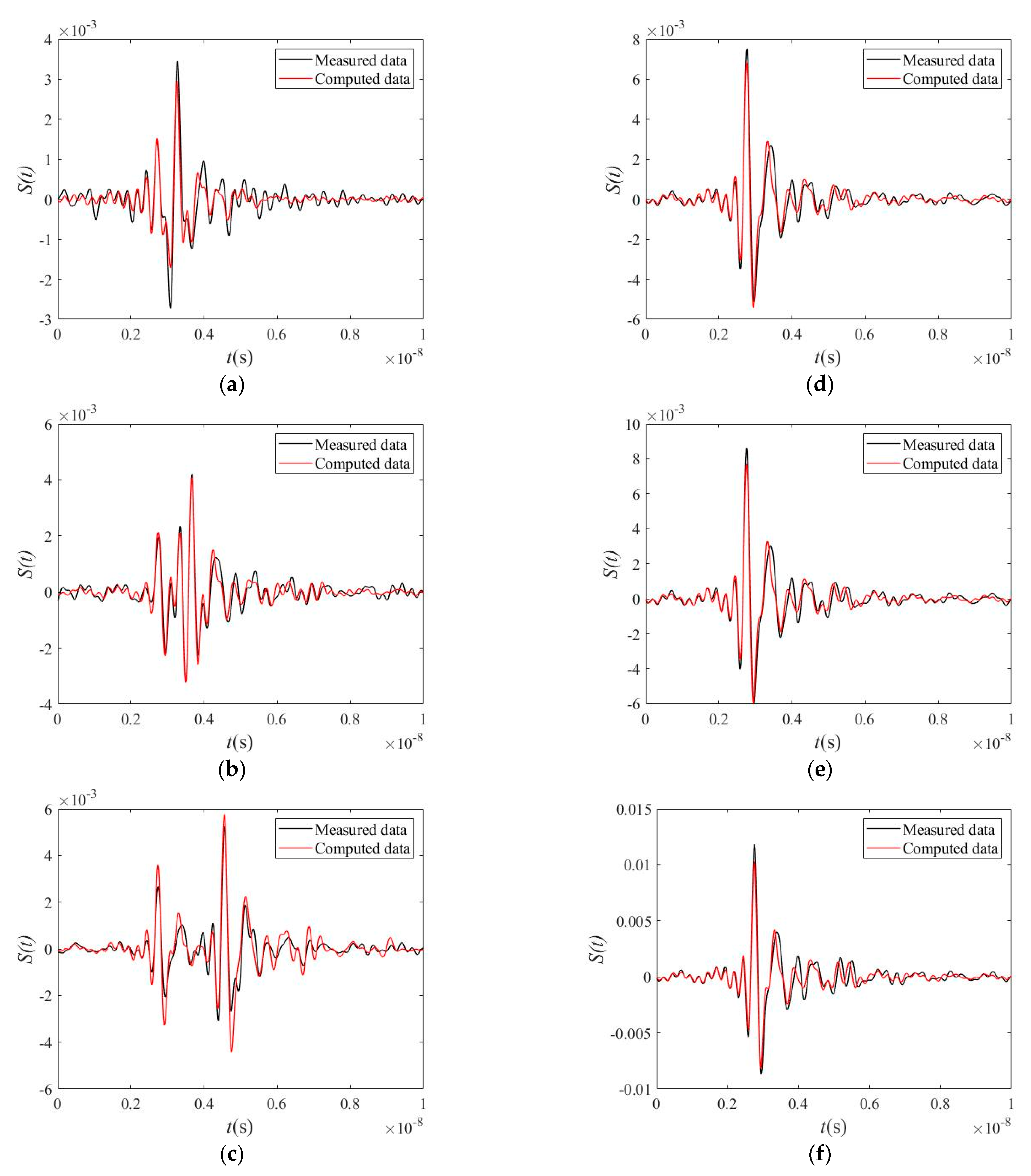
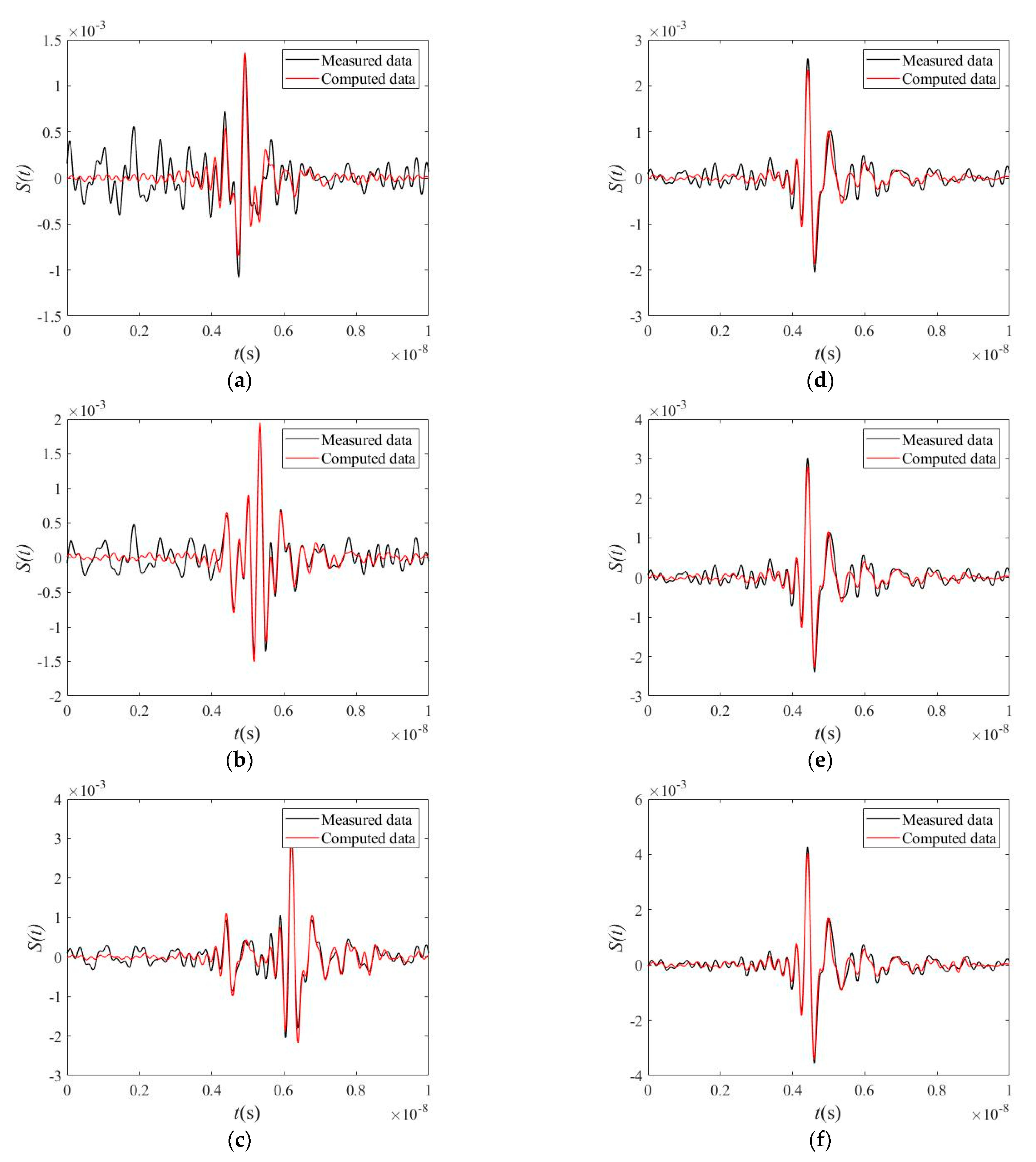
3.2. Full-Wave Inversion Analysis

3.2.1. Topography of the Objective Functions

In order to analyze the well posedness of the inverse problem to estimate the radius and permittivity of the laboratory models, we calculated the objective function distributions for all the six laboratory cylinders. For the nonconductive cylinders PVC-1, PVC-2, and PVC-3, the objective function was calculated, based on model 5. For the conductive cylinders Metal-1, Metal-2, and Metal-3, the objective function was calculated based on model 6.

Figure 7 shows the objective function of the three PVC pipe models filled with sand at two different positions. For the smallest nonconductive model PVC-1, the objective function distributions with respect to radius and relative permittivity at position 0.15 m and 0.4 m were almost the same except for the bounds. The relatively easy changing responses and the fact that there were no local minima indicated that retrieving the relative permittivity and radius at the same time for small nonconductive cylindrical media could, in principle, be feasible. The gradients near the global minimum were relatively small, depicting good stabilities of the inverse problem because even if there were noise in the measured data, the inversed parameters could still be around the real data. However, high-resolution inversion of these small radius cylindrical objects like PVC-1 is of great challenge, due to the ambiguity of the global minimum. To pursue a high-resolution detection for small radius cylinders, higher frequencies must be employed.

For the nonconductive cylindrical model PVC-2, the radius was 0.0406 m, although about two local minima emerged for each position, the global minimum was much smaller than the local minima and the gradients around the global minimum were very sharp. This demonstrates that in the frequency range 1–4 GHz, retrieving the radius and relative permittivity of a nonconductive cylinder with a radius of around 0.04 m could be relatively easy: well-defined minimum and relatively simple objective function topography. For the nonconductive cylindrical model PVC-3, the radius was 0.0801 m, several local minima occurred for both positions, indicating that inverting these large cylindrical objects in the frequency range 1–4 GHz could be easily trapped in the local minimum. However, the gradient of the objective function in correspondence to the global minima was much sharper than the gradient close to the local minimum. If we choose the inversion algorithms which have strong abilities to avoiding plunging into local minimum, inverting for both the radius and the relative permittivity for the large nonconductive cylindrical targets in the frequency range 1–4 GHz is theoretically possible.

For PVC-2 and PVC-3, when the distance between the antenna aperture and the cylinder was equal to 0.4 m, the gradients around the global minimum were sharper than those when the distance between the antenna aperture and the cylinder was equal to 0.15 m. This is mainly due to the fact that the far-field model is less applicable when the distance between the antenna aperture and the detected object is less than a threshold, which is defined as 1.2 times of the maximum dimension of the antenna aperture [53]. The presence of the local minimum indicates that for nonconductive cylindrical objects, the relative permittivity and radius are coupled. For smaller cylindrical objects like PVC-1, the coupling effect between the relative permittivity and radius also existed. We did not observe any local minimum for PVC-1 because in the frequency range 1–4 GHz, the resolution was not high enough to allow us to see more detailed results. In this condition, we think that more local minima will be brought to sight if we use larger frequency ranges (e.g., see De Coster, Tran and Lambot [54]).

Figure 8 shows the objective function with respect to the radius for a cylindrical metal model. For the distance d = 0.15 m, the minimum of the objective function for Metal-1, Metal-2 and Metal-3 occurred at radius 0.01 m, 0.01 m and 0.02 m, respectively. We think that these discrepancies between the model and the measurements mainly originate from the fact that we reached the limit of the signal-to-noise ratio. To encourage higher accuracy, higher frequencies would be needed. For the distance d = 0.4 m, the minimum of the objective function occurred at radius 0.01 m, 0.02 m and 0.06 m, respectively. For the conductive cylinders, when the position was 0.4 m, the minimum of the objective function was consistent with the real radius values. However, closer, the agreements were less satisfactory.

3.2.2. The Local Optimization Results

Table 2. The inversed parameters of the laboratory models at position 0.15 m.

Model	Radius (m)			Relative permittivity
	Estimated	Measured	Error (%)	Estimated	Measured
PVC-1	0.0236	0.0201	17.41	1.8428	2.35–2.82
PVC-2	0.0432	0.0406	6.40	2.0641	2.35–2.82
PVC-3	0.0801	0.0805	0.50	2.4316	2.35–2.82
Metal-1	0.0051	0.0170	70.00	/	/
Metal-2	0.0082	0.0248	66.93	/	/
Metal-3	0.0207	0.0640	67.66	/	/

and

Table 3. The inversed parameters of the laboratory models at position 0.4 m.

Model	Radius (m)			Relative permittivity
	Estimated	Real	Error (%)	Estimated	Measured
PVC-1	0.0210	0.0201	4.48	2.3283	2.35–2.82
PVC-2	0.0419	0.0406	3.20	2.2918	2.35–2.82
PVC-3	0.0815	0.0805	1.24	2.4057	2.35–2.82
Metal-1	0.0124	0.0170	27.06	/	/
Metal-2	0.0203	0.0248	18.15	/	/
Metal-3	0.0528	0.0640	17.50	/	/

show the inversion results for the six cylindrical models at distances 0.15 m and 0.4 m, respectively. For both positions, the estimated radius of the PVC-1, PVC-2 and PVC-3 targets were close to the measured value. The relative permittivity was estimated in a range from 1.8428 to 2.4316. For Metal-1, Metal-2 and Metal-3, the estimated radiuses were less satisfying for position 0.14 m than that of 0.4 m.

In laboratory conditions, the signal-to-noise ratio is, in general, relatively high. Retrieving the global minimum is not difficult, especially when the searched parameters in the lookup table are dense enough. However, we observed some discrepancies between the model and the measurements, especially for the cases where the backscattered signal from the cylinder was relatively small. In that respect, this could be improved by operating closer to the target and by using much higher frequency ranges. Besides, for nonconductive cylindrical media, the influence of relative permittivity and radius on the objective function is correlated, further increasing uncertainties in the retrieved parameters.

Figure 9 and Figure 10 show the measured time domain signal and the computed data using the inversion results at position 0.15 m and 0.4 m, respectively. At both positions, the measured and computed data matched quite well for the conductive cylindrical models. For the nonconductive cylindrical model, the computed amplitude of the first arrival and the second arrival matched well with the measured data. There was a slight mismatch before the first and also after the second arrival at position 0.15 m but this kind of mismatch at position 0.4 m was larger.

Both numerical and laboratory results indicate that the amplitude of the first reflection is a very important parameter for cylinder inversion. For conductive cylindrical media, because both the radius and the conductivity affect similarly the amplitude of the first reflection, it is difficult to retrieve these two parameters at the same time (highly correlated) as has been analyzed in Section 3.1. For the nonconductive cylindrical model, although there were greater relative mismatches before the first arrival compared to the conductive models, the retrieved radius and the relative permittivity still stayed in a normal range.

4. Conclusions

We addressed forward and inverse modeling of UWB radar data for wave propagation through cylindrical objects. In particular, we combined the radar equation of Lambot et al. [43,44,45,46,47,48,49] with cylindrical Green’s functions, which was initially validated only for planar layered media. Numerical analyses were performed to investigate the well posedness of the inverse problem and robustness of the inversion strategy, i.e., the lookup table approach combined with local optimization to refine the results. Assuming cylinders with a unique layer, the analysis of the topography of the objective function, as well as numerical inversions, demonstrated the uniqueness of the solution to retrieve the cylinder radius and permittivity. Nevertheless, the inverse problem becomes more complicated when electrical conductivity is also considered, due to correlations with the other parameters. Our numerical analysis results indicate that inverting for both the radius and electrical conductivity at the same time is not a good choice because these two parameters affect the radar signal in a very similar way. The presence of local minima in the objective functions also imposes the use of a global optimization strategy to find the global minimum of the objective function. For the conductive cylinders, the amplitude of the first arrival is increasing with both electrical conductivity and radius. The phase and amplitude of the second arrival are affected by the two parameters in a more complicated way. For small radius cylinders, we did not detect any local minimum in the objective function because the frequency range we employed was not high enough to allow us to see more detailed results, and the global minimum was quite flat. This makes it easy to inverse a coarse but stable result for small cylinders (radius is about 0.02 m) in the frequency range 1–4 GHz. For the cylinders with an intermediate or larger radius, the global minimum was very well defined. Yet, several local minima occurred because the radius and the relative permittivity were partly correlated in the inverse problem. We believe that more local minimum will be brought to sight if larger frequency ranges are employed. For the conductive cylindrical media, both the radius and the conductivity were highly correlated as they both affected similarly the amplitude of the reflections. These two parameters are therefore complicated to retrieve.

The laboratory results demonstrated that, in far-field conditions, the model accurately represents real radar data. Nevertheless, when the cylinder has a relatively small diameter and small reflection coefficient at its surface, leading to a relatively weak backscattered signal, modeling results are less satisfactory due to the limited signal-to-noise ratio. In that case, operating closer to the target and using higher frequency ranges become necessary. Future research will focus on near-field modeling of radar data for improving the accuracy of the reconstructions. In the meantime, our methods will be tested on more complicated structures, with the goal of enhancing the inversion method to use FWI in more areas, such as tree trunk inspection and concrete column testing.

References

1. Liu, X.; Dong, X.; Xue, Q.; Leskovar, D.I.; Jifon, J.; Butnor, J.R.; Marek, T. Ground penetrating radar (GPR) detects fine roots of agricultural crops in the field. Plant Soil 2018, 423, 517–531. [Google Scholar] [CrossRef]
2. Benedetto, A.; Pajewski, L. Civil Engineering Applications of Ground Penetrating Radar; Springer: Cham, Switzerland, 2015. [Google Scholar]
3. Pälli, A.; Kohler, J.C.; Isaksson, E.; Moore, J.C.; Pinglot, J.F.; Pohjola, V.A.; Samuelsson, H. Spatial and temporal variability of snow accumulation using ground-penetrating radar and ice cores on a Svalbard glacier. J. Glaciol. 2002, 48, 417–424. [Google Scholar] [CrossRef] [Green Version]
4. Arcone, S.A.; Lawson, D.E.; Delaney, A.J.; Strasser, J.C.; Strasser, J.D. Ground-Penetrating Radar Reflection Profiling of Groundwater and Bedrock in an Area of Discontinuous Permafrost. Geophysics 1998, 63, 1573–1584. [Google Scholar] [CrossRef]
5. Böniger, U.; Tronicke, J. Improving the interpretability of 3D GPR data using target–specific attributes: Application to tomb detection. J. Archaeol. Sci. 2010, 37, 672–679. [Google Scholar] [CrossRef]
6. Neal, A.; Roberts, C.L. Applications of Ground-Penetrating Radar (GPR) to Sedimentological, Geomorphological and Geoarchaeological Studies in Coastal Environments; Geological Society, Special Publications: London, UK, 2000; Volume 175, pp. 139–171. [Google Scholar]
7. Daniels, D.J. A review of GPR for landmine detection. Sens. Imag. Int. J. 2006, 7, 90–123. [Google Scholar] [CrossRef]
8. Zhu, Q.; Collins, L. Application of feature extraction methods for landmine detection using the Wichmann/Niitek ground-penetrating radar. IEEE Trans. Geosci. Remote Sens. 2005, 43, 81–85. [Google Scholar] [CrossRef]
9. Torrione, P.; Collins, L.M. Texture Features for Antitank Landmine Detection Using Ground Penetrating Radar. IEEE Trans. Geosci. Remote Sens. 2007, 45, 2374–2382. [Google Scholar] [CrossRef]
10. Ježová, J.; Mertens, L.; Lambot, S. Ground-penetrating radar for observing tree trunks and other cylindrical objects. Constr. Build. Mater. 2016, 123, 214–225. [Google Scholar] [CrossRef]
11. Devaru, D.; Halabe, U.B.; Gopalakrishnan, B.; Agrawal, S.; Grushecky, S. Algorithm for detecting defects in wooden logs using ground penetrating radar. Proc. Spie Int. Soc. Opt. Eng. 2005, 5999, 835. [Google Scholar] [CrossRef]
12. Tetuko, J.; Tateishi, R.; Wikantika, K. A method to estimate tree trunk diameter and its application to discriminate Java-Indonesia tropical forests. Int. J. Remote Sens. 2001, 22, 177–183. [Google Scholar] [CrossRef]
13. Giannakis, I.; Tosti, F.; Lantini, L.; Alani, A.M. Health Monitoring of Tree Trunks Using Ground Penetrating Radar. IEEE Trans. Geosci. Remote Sens. 2019, 57, 8317–8326. [Google Scholar] [CrossRef]
14. Boero, F.; Fedeli, A.; Lanini, M.; Maffongelli, M.; Monleone, R.; Pastorino, M.; Randazzo, A.; Salvadè, A.; Sansalone, A. Microwave Tomography for the Inspection of Wood Materials: Imaging System and Experimental Results. IEEE Trans. Microw. Theory Tech. 2018, 66, 3497–3510. [Google Scholar] [CrossRef]
15. Alani, A.M.; Soldovieri, F.; Catapano, I.; Giannakis, I.; Gennarelli, G.; Lantini, L.; Ludeno, G.; Tosti, F. The Use of Ground Penetrating Radar and Microwave Tomography for the Detection of Decay and Cavities in Tree Trunks. Remote Sens. 2019, 11, 2073. [Google Scholar] [CrossRef] [Green Version]
16. Li, C.; Tofighi, M.-R.; Schreurs, D.; Horng, T.-S.J. Principles and Applications of RF/Microwave in Healthcare and Biosensing; Academic Press: New York, NY, USA, 2017. [Google Scholar]
17. Conceição, R.C.; Medeiros, H.; Godinho, D.M.; O’Halloran, M.; Rodriguez-Herrera, D.; Flores-Tapia, D.; Pistorius, S. Classification of breast tumor models with a prototype microwave imaging system. Med. Phys. 2020, 47, 1860–1870. [Google Scholar] [CrossRef] [PubMed]
18. Dachena, C.; Fedeli, A.; Fanti, A.; Lodi, M.B.; Pastorino, M.; Randazzo, A. Microwave Imaging for the Diagnosis of Cervical Diseases: A Feasibility Analysis. IEEE J. Electromagn. RF Microw. Med. Biol. 2020, in press. [Google Scholar] [CrossRef]
19. Fedeli, A.; Schenone, V.; Randazzo, A.; Pastorino, M.; Henriksson, T.; Semenov, S. Nonlinear S-Parameters Inversion for Stroke Imaging. IEEE Trans. Microw. Theory Tech. 2021, 69, 1760–1771. [Google Scholar] [CrossRef]
20. Gennarelli, G.; Ludeno, G.; Catapano, I.; Soldovieri, F. Full 3-D Imaging of Vertical Structures via Ground-Penetrating Radar. IEEE Trans. Geosci. Remote Sens. 2020, 58, 8857–8873. [Google Scholar] [CrossRef]
21. Negishi, T.; Gennarelli, G.; Soldovieri, F.; Liu, Y.; Erricolo, D. Radio Frequency Tomography for Nondestructive Testing of Pillars. IEEE Trans. Geosci. Remote Sens. 2020, 58, 3916–3926. [Google Scholar] [CrossRef]
22. Pastorino, M.; Randazzo, A. Microwave Imaging Methods and Applications; Artech House: Norwood, MA, USA, 2018. [Google Scholar]
23. Jezova, J.; Harou, J.; Lambot, S. Reflection waveforms occurring in bistatic radar testing of columns and tree trunks. Constr. Build. Mater. 2018, 174, 388–400. [Google Scholar] [CrossRef]
24. Li, W.; Wen, J.; Xiao, Z.; Xu, S. Application of Ground-Penetrating Radar for Detecting Internal Anomalies in Tree Trunks with Irregular Contours. Sensors 2018, 18, 649. [Google Scholar] [CrossRef] [Green Version]
25. Kiat, T.T.W.; Rahiman, M.H.F.; Jack, S.P. An initial study to investigate the potential of microwave tomography for agarwood imaging. Int. J. Agric. For. Plant. 2016, 4, 26–32. [Google Scholar]
26. Chew, W.C. Waves and Fields in Inhomogenous Media; IEEE Press: Piscataway, NY, USA, 1995. [Google Scholar]
27. Roberts, R.L.; Daniels, J.J. Modeling near-field GPR in three dimensions using the FDTD method. Geophysics 1997, 62, 1114–1126. [Google Scholar] [CrossRef]
28. Semenov, S.; Bulyshev, A.; Abubakar, A.; Posukh, V.; Sizov, Y.; Souvorov, A.; Berg, P.V.D.; Williams, T. Microwave-tomographic imaging of the high dielectric-contrast objects using different image-reconstruction approaches. IEEE Trans. Microw. Theory Tech. 2005, 53, 2284–2294. [Google Scholar] [CrossRef]
29. Scapaticci, R.; Catapano, I.; Crocco, L. Wavelet-Based Adaptive Multiresolution Inversion for Quantitative Microwave Imaging of Breast Tissues. IEEE Trans. Antennas Propag. 2012, 60, 3717–3726. [Google Scholar] [CrossRef]
30. Lovell, J.R.; Chew, W.C. Response of a Point Source in a Multicylindrcally Layered Medium. IEEE Trans. Geosci. Remote Sens. 1987, GE-25, 850–858. [Google Scholar] [CrossRef]
31. Liu, Q. Electromagnetic field generated by an off-axis source in a cylindrically layered medium with an arbitrary number of horizontal discontinuities. Geophysics 1993, 58, 616–625. [Google Scholar] [CrossRef]
32. Wait, J.R. Electromagnetic Radiation from Cylindrical Structures; The Institution of Electrical Engineers: London, UK, 1988. [Google Scholar]
33. Wait, J.R.; Hill, D.A. Excitation of a homogeneous conductive cylinder of finite length by a prescribed axial current distribution. Radio Sci. 1973, 8, 1169–1176. [Google Scholar] [CrossRef]
34. Wu, J.; Khamas, S.K.; Cook, G.G. An Efficient Asymptotic Extraction Approach for the Green’s Functions of Conformal Antennas in Multilayered Cylindrical Media; IEEE Transactions on Antennas and Propagation: Piscataway, NJ, USA, 2010; Volume 58, pp. 3737–3742. [Google Scholar]
35. Zhonggui, X.; Yilong, L. Electromagnetic dyadic Green’s function in cylindrically multilayered media. IEEE Trans. Microw. Theory Tech. 1996, 44, 614–621. [Google Scholar] [CrossRef]
36. Fedeli, A.; Pastorino, M.; Raffetto, M.; Randazzo, A. 2-D Green’s Function for Scattering and Radiation Problems in Elliptically Layered Media With PEC Cores. IEEE Trans. Antennas Propag. 2017, 65, 7110–7118. [Google Scholar] [CrossRef]
37. Tokgoz, C.; Dural, G. Closed-form Green’s functions for cylindrically stratified media. IEEE Trans. Microw. Theory Tech. 2000, 48, 40–49. [Google Scholar] [CrossRef]
38. Sun, J.; Wang, C.-F.; Li, L.-W.; Leong, M.-S. A Complete Set of Spatial-Domain Dyadic Green’s Function Components for Cylindrically Stratified Media in Fast Computational Form. J. Electromagn. Waves Appl. 2002, 16, 1491–1509. [Google Scholar] [CrossRef]
39. Ye, L.-F.; Zhao, F.; Xiao, K.; Chai, S.-L. A Robust Method for the Computation of Green’s Functions in Cylindrically Stratified Media’. IEEE Trans. Antennas Propag. 2012, 60, 3046–3051. [Google Scholar] [CrossRef]
40. Bhattacharya, D.; Ghosh, B.; Sarabandi, K. Evaluation of Efficient Closed-Form Green’s Function in a Cylindrically Stratified Medium. IEEE Trans. Antennas Propag. 2017, 65, 1505–1510. [Google Scholar] [CrossRef]
41. Karan, S.; Ertürk, V.B.; Altintas, A. Closed-Form Green’s Function Representations in Cylindrically Stratified Media for Method of Moments Applications. IEEE Trans. Antennas Propag. 2009, 57, 1158–1168. [Google Scholar] [CrossRef] [Green Version]
42. Ye, L.F.; Xiao, K.; Qiu, L.; Chai, S.-L.; Mao, J.-J. An Efficient Method for the Computation of Mixed Potential Green’s Functions in Cylindrically Stratified Media. Prog. Electromagn. Res. 2012, 125, 37–53. [Google Scholar] [CrossRef] [Green Version]
43. Warren, C.; Giannopoulos, A.; Giannakis, I. gprMax: Open source software to simulate electromagnetic wave propagation for Ground Penetrating Radar. Comput. Phys. Commun. 2016, 209, 163–170. [Google Scholar] [CrossRef] [Green Version]
44. Lambot, S.; Slob, E.; Bosch, I.V.D.; Stockbroeckx, B.; Vanclooster, M. Modeling of ground-penetrating Radar for accurate characterization of subsurface electric properties. IEEE Trans. Geosci. Remote Sens. 2004, 42, 2555–2568. [Google Scholar] [CrossRef]
45. Lambot, S.; Andre, F. Full-Wave Modeling of Near-Field Radar Data for Planar Layered Media Reconstruction. IEEE Trans. Geosci. Remote Sens. 2014, 52, 2295–2303. [Google Scholar] [CrossRef]
46. Ježová, J.; Lambot, S. A dielectric horn antenna and lightweight radar system for material inspection. J. Appl. Geophys. 2019, 170, 3822. [Google Scholar] [CrossRef]
47. Aksun, M.I.; Dural, G. Clarification of issues on the closed-form Green’s functions in stratified media. IEEE Trans. Antennas Propag. 2005, 53, 3644–3653. [Google Scholar] [CrossRef]
48. Simsek, E.; Qing Huo, L.; Baojun, W. Singularity subtraction for evaluation of Green’s functions for multilayer media. IEEE Trans. Microw. Theory Tech. 2006, 54, 216–225. [Google Scholar] [CrossRef]
49. He, X.; Gong, S.; Liu, Q. Fast computation of spatial Green’s functions of multilayered microstrip antennas. Microw. Opt. Technol. Lett. 2005, 45, 85–88. [Google Scholar] [CrossRef]
50. Lambot, S.; Slob, E.; Vereecken, H. Fast evaluation of zero-offset Green’s function for layered media with application to ground-penetrating radar. Geophys. Res. Lett. 2007, 34, 21. [Google Scholar] [CrossRef] [Green Version]
51. De Coster, A.; Lambot, S. Full-Wave Removal of Internal Antenna Effects and Antenna–Medium Interactions for Improved Ground-Penetrating Radar Imaging. IEEE Trans. Geosci. Remote Sens. 2018, 57, 93–103. [Google Scholar] [CrossRef]
52. Lagarias, J.C.; Reeds, J.A.; Wright, M.H.; Wright, P.E. Convergence Properties of the Nelder--Mead Simplex Method in Low Dimensions. SIAM J. Optim. 1998, 9, 112–147. [Google Scholar] [CrossRef] [Green Version]
53. Tran, A.P.; André, F.; Craeye, C.; Lambot, S. Near-Field Or Far-Field Full-Wave Ground Penetrating Radar Modeling As A Function Of The Antenna Height Above A Planar Layered Medium. Prog. Electromagn. Res. 2013, 141, 415–430. [Google Scholar] [CrossRef] [Green Version]
54. De Coster, A.; Tran, A.P.; Lambot, S. Fundamental Analyses on Layered Media Reconstruction Using GPR and Full-Wave Inversion in Near-Field Conditions. IEEE Trans. Geosci. Remote Sens. 2016, 54, 5143–5158. [Google Scholar] [CrossRef]
Figure 1. Schematic representation of the considered cylindrically layered medium.
Remotesensing 13 02370 g001
Figure 2. Model configuration for numerical experiments.
Remotesensing 13 02370 g002
Figure 3. Detecting the cylindrical model with the lightweight radar system with vertical polarization.
Remotesensing 13 02370 g003
Figure 4. Amplitude and phase of the (a) return loss transfer function (b) global transmission and reflection coefficient function and (c) feedback loss transfer function of the BBHA 9120D horn antenna as a function of frequency.
Remotesensing 13 02370 g004
Figure 5. The effects of (a) radius and (b) relative permittivity on nonconductive cylindrical models.
Remotesensing 13 02370 g005
Figure 6. The effects of (a) radius and (b) conductivity on conducting cylindrical models.
Remotesensing 13 02370 g006
Figure 7. The objective function distribution of (a) PVC-1 with d equals 0.15 m, (b) PVC-2 with d equals 0.15 m, (c) PVC-3 with d equals 0.15 m, (d) PVC-1 with d equals 0.4 m, (e) PVC-2 with d equals 0.4 m, (f) PVC-3 with d equals 0.4 m.
Remotesensing 13 02370 g007
Figure 8. The objective function distributions of metallic tubes with distances of (a) 0.15 m and (b) 0.4 m.
Remotesensing 13 02370 g008
Figure 9. The comparison between the measured time domain signal and the modeled time domain signal of (a) PVC-1, (b) PVC-2, (c) PVC-3, (d) Metal-1, (e) Metal-2, (f) Metal-3 at position 0.15 m.
Remotesensing 13 02370 g009
Figure 10. The comparison between the measured time domain signal and the computed time domain signal of (a) PVC-1, (b) PVC-2, (c) PVC-3, (d) Metal-1, (e) Metal-2, (f) Metal-3 at position 0.4 m.
Remotesensing 13 02370 g010