Oil Spill Detection with Multiscale Conditional Adversarial Networks with Small-Data Training

Abstract

We investigate the problem of training an oil spill detection model with small data. Most existing machine-learning-based oil spill detection models rely heavily on big training data. However, big amounts of oil spill observation data are difficult to access in practice. To address this limitation, we developed a multiscale conditional adversarial network (MCAN) consisting of a series of adversarial networks at multiple scales. The adversarial network at each scale consists of a generator and a discriminator. The generator aims at producing an oil spill detection map as authentically as possible. The discriminator tries its best to distinguish the generated detection map from the reference data. The training procedure of MCAN commences at the coarsest scale and operates in a coarse-to-fine fashion. The multiscale architecture comprehensively captures both global and local oil spill characteristics, and the adversarial training enhances the model’s representational power via the generated data. These properties empower the MCAN with the capability of learning with small oil spill observation data. Empirical evaluations validate that our MCAN trained with four oil spill observation images accurately detects oil spills in new images.

1. Introduction

Frequent oil spill accidents have caused great harm to marine life and national economies in recent years. Accurately detecting oil spills in remote sensing images plays an important role in environmental protection and emergency responses for marine accidents. Among the many monitoring methods that use remote sensing, synthetic aperture radar (SAR) is an essential tool for observing oil spills with its broad view and all-time and all-weather data acquisition [1,2,3]. Oil spill detection based on SAR images is an indispensable research topic in the field of ocean remote sensing [4,5,6,7].

The principle of oil spill detection lies in the differential display between oil and water in oil spill observation images [8,9]. As oil spills can weaken the Bragg scattering and result in dark regions in the observation images, numerous researchers are dedicated to analyzing the physical characteristics of oil spills. In particular, the polarimetric characteristics have been effectively used to enhance the comprehensive observation effect [10,11]. Moreover, other kinds of techniques for oil spill detection based on semplice image processing have mainly drawn support from energy minimization [12], which is the optimization objective of energy functions.

Mdakane and Kleynhans [5] achieved efficient oil spill detection with an automatic segmentation framework that combines automated threshold-based and region-based algorithms. Ren et al. [13] took the shapes of elongated oil spills and their details into consideration with a dual-smoothing framework that operates at both the label and pixel levels. Ren et al. [14] proposed a solution to the problem of manual labeling with one-dot fuzzy initialization. Chen et al. [15] exploited a segmentation method with multipliers of alternating directions to handle blurry SAR images. Energy-minimization-based segmentation is not too computationally expensive, but relies heavily on the initialization information; such information is usually scarce, as it is provided by manually segmented images.

Machine-learning-based oil spill detection models have been investigated extensively in recent years, as they have been proven to have the ability to intelligently extract the internal information of SAR images. Inchoate detection models tend to find oil spills in three steps [16,17,18,19,20,21]: dark-spot detection, feature extraction, and dark-spot classification. An early machine-learning-based model used adaptive thresholding for dark-spot detection and extracted four features in order to conduct the subsequent dark-spot classification [4]. Brekke and Solberg [22] developed an improved two-step classification procedure for oil spill detection in SAR images, consisting of a regularized statistical classifier and an automatic confidence estimation of the detected slicks. Singha et al. [23] employed two different artificial neural networks (ANNs) in sequence; the first ANN outputs candidate pixels belonging to oil spills, and the corresponding feature parameters drive the second ANN to classify objects into oil spills or lookalikes. Xu et al. [24] made a comparative study of classification techniques by analyzing classifiers, including support vector machines, artificial neural networks, tree-based ensemble classifiers (bagging, bundling, and boosting), generalized additive models, and penalized linear discriminant analysis. Taravat et al. [25] proposed an automated dark-spot detection approach combining the Weibull multiplicative model and pulse-coupled neural network techniques; the proposal differentiates between dark spots and background.

Machine-learning-based methods use step-by-step operations and can seldom be implemented as end-to-end detection pipelines. Such stepwise schemes rely on complex procedures and do not guarantee efficient oil spill detection.

Recently, deep learning has been investigated for target recognition [2,26] and oil spill detection [27,28,29]. Gallego et al. [30] used a deep residual encoder–decoder network for oil spill detection in one step. The encoder receives the input image and creates a latent representation, and the decoder takes this intermediate representation and outputs the oil spill detection results. Nieto-Hidalgo et al. [31] proposed a two-stage convolutional neural network to detect oil spills from side-looking airborne radar images. The first network performs a coarse detection, and the second one provides a precise pixel classification. Shaban et al. [32] used a two-stage deep learning framework that considers the unbalanced nature of datasets for oil spill identification. The first network classifies oil spill image patches via a 23-layer convolutional neural network, and the second network performs semantic segmentation using a five-stage U-Net. Li et al. [33] discussed two automatic detection models that combine a fully convolutional network (FCN) [34] with Resnet [35] and Googlenet [36] for oil spill images, with no restrictions on the size of the input. These methods achieve effective detection in an end-to-end fashion, and they tend to outperform ordinary machine-learning-based methods.

Other approaches for the same purpose employ adversarial training mechanisms, including generative adversarial networks (GANs) [37,38,39,40,41] and conditional adversarial networks (CANs) [42,43]. CANs are capable of learning the transformation of observation images into detection maps in accordance with the users’ expectations. Yu et al. [44] used a detection model with adversarial f-divergence learning for automatic oil spill identification. The network utilized in adversarial f-divergence learning is a typical CAN. CAN-based oil spill detection methods are reliable and achieve good accuracy.

The intelligent detection methods described above are driven by a training process. Most machine-learning-based oil spill detection methods depend on large amounts of training data to guarantee accurate detection results. Significant amounts of oil spill observation data are challenging to obtain, and training an oil spill detection model with small amounts of data remains a challenge in the literature. To eliminate the dependence on vast observation data of oil spills, we developed a multiscale conditional adversarial network (MCAN) to achieve such a goal with small amounts of training data.

MCAN consists of a series of adversarial networks at multiple scales. Both images of observed oil spills and detection maps are used in coarse-to-fine representations at multiple scales. Each adversarial network of the MCAN at each scale is composed of a generator and a discriminator. The generator captures the observed image’s characteristics and produces an oil spill detection map as authentically as possible. The discriminator distinguishes the generated detection map from the reference data. The output of each generator is used as the input of the following finer-scale generator and the current-scale discriminator. The training procedure of each scale is conducted independently in an adversarial fashion.

The three features (i.e., (i) multiscale processing, (ii) coarse-to-fine data flow in a cascade, and  (iii) independent adversarial training) enable MCAN to comprehensively capture data characteristics, and they empower it with the capability of learning with small amounts of data. The experimental results validate that MCAN produces accurate detection maps for sophisticated oil spill regions based on only four training data samples. The detection performance of MCAN outperforms those of other methods.

The main contributions of this article are summarized as follows.

• We propose a novel oil spill detection method based on MCAN, which employs a lightweight network for each generator and discriminator.
• We implement adversarial training independently at each scale and achieve a coarse-to-fine data flow of oil spill features in a cascade.
• We elaborately set small training data with different characteristics to conduct an experimental evaluation.

The rest of this article is structured as follows. Section 2 describes our MCAN framework and presents the training procedure. Section 3 provides the experimental settings and evaluations. Section 4 discusses the experimental results. Finally, Section 5 presents conclusions about the proposed method and its performance.

2. Materials and Methods

Adversarial learning with one generator and one discriminator is widely used in the task of semantic segmentation. The generator is trained by a loss function that is automatically learned from the discriminator. The discriminator learns the distribution between the real and generated maps, allowing for flexible losses and alleviating the need for manual tuning.

Oil spill detection with small-data training is a promising and practically significant learning method. It requires a well-designed network and, in the case under study, an efficient training mode in order to learn an effective oil spill detection model. Adversarial learning is adequate for small-data training. This section describes how to detect oil spills via a multiscale conditional adversarial network (MCAN) trained with few samples.

2.1. The MCAN Architecture

We denote an oil spill observation image as $I_0$, the reference data of the oil spill region as $S_0$, and  the corresponding oil spill detection map produced by the MCAN as ${\widehat{S}}_0$. Both $S_0$ and ${\widehat{S}}_0$ are binary images in which 0 represents the oil spill and 1 represents the ocean surface. We establish multiscale representations for $I_0$, $S_0$, and ${\widehat{S}}_0$, starting from the 0-th scale.

The representations $I_n$ and $S_n$ at the n-th scale are obtained by downsampling (by averaging values) the 0-th-scale data by a factor $r^n$, where r is usually set to 2. We denote by $G_n$ the n-th generator network, which produces ${\widehat{S}}_n$. The size of ${\widehat{S}}_n$ is $1/r^n$ of that of ${\widehat{S}}_0$, and ${\widehat{S}}_n$ is considered as the n-th-scale representation for ${\widehat{S}}_0$. Representations across $N+1$ scales from the N-th scale to the 0-th scale form the coarse-to-fine multiscale representation set that is used in the MCAN oil spill detection.

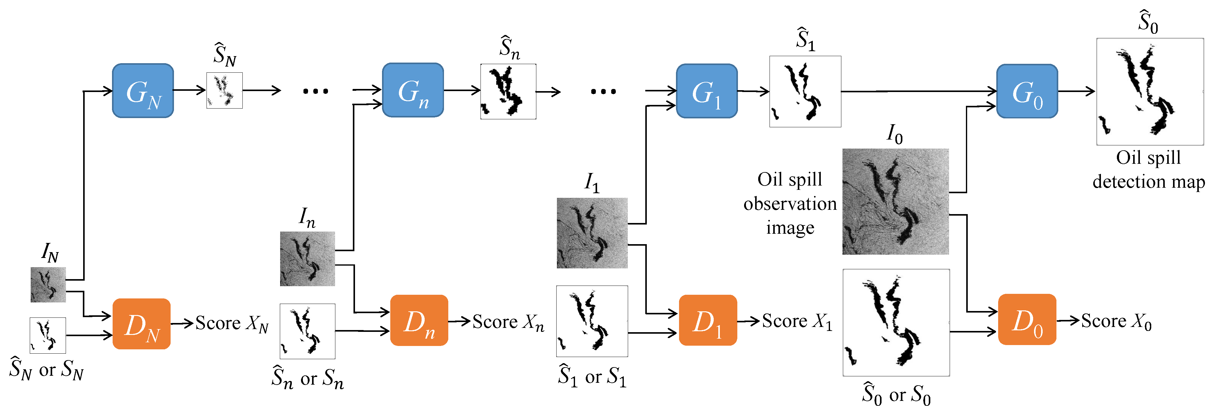
We propose a multiscale conditional adversarial network consisting of a series of generators and discriminators at multiple scales. The generator $G_n$ and the discriminator $D_n$ process representations at the n-th scale.

Figure 1 illustrates the architecture of MCAN. The oil spill observation image $I_0$ and the oil spill detection map ${\widehat{S}}_0$ are the input and output of the overall MCAN framework, respectively. The generator $G_n$ takes both the oil spill observation image $I_n$ at the n-th scale and the generated oil spill detection map ${\widehat{S}}_{n+1}$ at the $(n+1)$-th scale as input and produces the generated oil spill detection map ${\widehat{S}}_n$ as the output. The discriminator $D_n$ takes $(I_n,S_n)$ or $(I_n,{\widehat{S}}_n)$ as input, and it separately outputs the corresponding discriminant scores. $D_n$ aims to distinguish between the reference oil spill detection map $S_n$ and the generated oil spill detection map ${\widehat{S}}_n$.

Figure 2 shows the architecture of the generator $G_n$ at the n-th scale. The inputs of $G_n$ are the observation image $I_n$ and the detection map ${\widehat{S}}_{n+1}$ from the $(n+1)$-th scale. By upsampling ${\widehat{S}}_{n+1}$ by a factor r, we obtain ${\widehat{S}}_{n+1}^{\uparrow }$ with the same size of $I_n$. The convolutional network $C_n$ processes the pair $\left(I_n,{\widehat{S}}_{n+1}^{\uparrow }\right)$ with five convolutional blocks. Each block consists of three layers, including a convolutional layer, a batch normalization (BN) layer, and a LeakyReLU (or Tanh) layer. The sum of the convolutional network’s output and ${\widehat{S}}_{n+1}^{\uparrow }$ forms the output of $G_n$, i.e., an oil spill detection map ${\widehat{S}}_n$ at the n-th scale. The operation within $G_n$ is:

$${\widehat{S}}_n=G_n(I_n,{\widehat{S}}_{n+1})=C_n(I_n,{\widehat{S}}_{n+1}^{\uparrow })+{\widehat{S}}_{n+1}^{\uparrow },n<N.$$

(1)

The sum $C_n(I_n,{\widehat{S}}_{n+1}^{\uparrow })+{\widehat{S}}_{n+1}^{\uparrow }$ is a typical residual learning scheme that enhances the representational power of the convolutional network. At the n-th scale, the generator $G_n$ aims to produce the oil spill detection map ${\widehat{S}}_n$ as authentically as possible.

At the coarsest scale, the generator $G_N$ only takes the oil spill observation image $I_N$ as input and outputs its oil spill detection map ${\widehat{S}}_N$, which is represented as follows:

$${\widehat{S}}_N=G_N\left(I_N\right)=C_N\left(I_N\right).$$

(2)

Figure 3 shows the architecture of the discriminator $D_n$ at the n-th scale. The network used in $D_n$ has five convolutional blocks. Each of the first four blocks has a convolutional layer, a batch normalization (BN) layer, and a LeakyReLU layer. The fifth one only has a convolutional layer.

The input of $D_n$ is either $\left(I_n,{\widehat{S}}_n\right)$ or $\left(I_n,S_n\right)$. The output of $D_n$ is a discriminant score $X_n$ that reflects the confidence on the detection map:

$$\begin{array}{c}\hfill X_n=\left\{\begin{array}{cc}{D}_n(I_n,{\widehat{S}}_n)\hfill & \mathrm{for}\mathrm{generated}{\widehat{S}}_n\mathrm{as}\mathrm{input},\hfill \\ D_n(I_n,S_n)\hfill & \mathrm{for}\mathrm{reference}\mathrm{data}{S}_n\mathrm{as}\mathrm{input},\hfill \end{array}\right.\end{array}$$

(3)

where $X_n$ is the average of the feature map $F_n$ that is output from $D_n$’s final convolutional layer. Each element of $F_n$ corresponds to a patch of the input image. The last output of $D_n$ integrates all of the elements of $F_n$ and aims to classify if each patch in the input image is real or generated. $D_n$ penalizes the generated pair $\left(I_n,{\widehat{S}}_n\right)$ and favors the actual pair $\left(I_n,S_n\right)$. At the n-th scale, the discriminator $D_n$ tries to distinguish the generated ${\widehat{S}}_n$ from the reference data $S_n$.

2.2. Training MCAN

The training of MCAN is conducted hierarchically from the N-th scale to the 0-th scale. At each scale, the training is performed independently in the same manner using a Wasserstein GAN–gradient penalty (WGAN-GP) loss [39] for stable training. Once the training at the $(n+1)$-th scale has concluded, the generated detection map ${\widehat{S}}_{n+1}$ is used for the training at the n-th scale.

The training loss for the generator $G_n$ is:

$$L_{G_n}={\lambda }_1\parallel S_n-{\widehat{S}}_n{\parallel }_1-D_n(I_n,{\widehat{S}}_n),$$

(4)

where ${\lambda }_1$ is a balance parameter. The term $-D_n(I_n,{\widehat{S}}_n)$ is the adversarial loss that encourages $G_n$ to generate a detection map ${\widehat{S}}_n$ that is as close as possible to the reference data $S_n$. The term $\parallel S_n-{\widehat{S}}_n{\parallel }_1$ is the ${\ell }_1$ norm loss. It penalizes the per-pixel distance between the reference data $S_n$ and the generated ${\widehat{S}}_n$. Minimizing (4) trains $G_n$ to generate detection maps as authentically as possible, and finally, they successfully fool the discriminator.

The training loss for the discriminator $D_n$ is given as:

$$\begin{array}{c}\hfill L_{D_n}=D_n(I_n,{\widehat{S}}_n)-D_n(I_n,S_n)+{\lambda }_2{\left(\parallel {\nabla }_{{\tilde{S}}_n}{D}_n(I_n,{\tilde{S}}_n){\parallel }_2-1\right)}^2,\end{array}$$

(5)

where ${\lambda }_2$ is a balance parameter, and ${\tilde{S}}_n$ denotes a random variable that samples uniformly between ${\widehat{S}}_n$ and $S_n$. The term $D_n(I_n,{\widehat{S}}_n)-D_n(I_n,S_n)$ represents the adversarial loss that strengthens the discrimination power of $D_n$; it makes $D_n$ try its best to classify ${\widehat{S}}_n$ as false and $S_n$ as true. The term $(\parallel {\nabla }_{{\tilde{S}}_n}{D}_n(I_n,{\tilde{S}}_n){{\parallel }_2-1)}^2$ is the gradient penalty loss. It results in stable gradients that neither vanish nor explode [39]. Minimizing (5) trains $D_n$ to distinguish the generated detection map from the reference data.

The training procedure of the proposed MCAN is described in Algorithm 1. The input consists of original SAR images and their corresponding reference data of oil spill detection results. The output is the trained parameter set of MCAN. For example, consider the training sample $I_0$ and its reference data $S_0$. If MCAN is set to have three scales, $I_0$ and $S_0$ are downsampled to obtain $(I_1,S_1)$ and $(I_2,S_2)$. The training procedure is conducted from generator $G_2$ and discriminator $D_2$. Firstly, the output of $G_2$ is computed by ${\widehat{S}}_2=G_2\left(I_2\right)$. Secondly, $D_2$ takes $S_2$ and ${\widehat{S}}_2$ separately as input. The parameters of $D_2$ are updated by Equation (5), and the parameters of $G_2$ are updated according to Equation (4). Thirdly, ${\widehat{S}}_2$ and $I_1$ are concatenated as the input of $G_1$ to obtain the output ${\widehat{S}}_1=G_1(I_1,{\widehat{S}}_2)$. $D_1$ and $G_1$ are updated as Equation (5) and Equation (4), respectively. Finally, ${\widehat{S}}_1$ and $I_0$ are concatenated as the input of $G_0$ to obtain the output ${\widehat{S}}_0=G_0(I_0,{\widehat{S}}_1)$. $D_0$ and $G_0$ are updated by Equations (5) and (4), respectively. At this point, the two images $I_0$ and $S_0$ go through one training iteration to update the parameters of MCAN. The next training sample pair will follow the same procedure as that for $I_0$ and $S_0$.

Algorithm 1 Training Procedure of the Proposed MCAN Oil Spill Detection Method.

Input: The training set consisting of original SAR images and their corresponding reference data of oil spill detection results Output: The trained parameter set of MCAN

for all training epochs do     for all scales do         Input a downsampled sample $I_n$ and ${\widehat{S}}_{n+1}$ from the $(n+1)$-th scale         Compute ${\widehat{S}}_n=G_n(I_n,{\widehat{S}}_{n+1})$         train $D_n$: Compute $L_{D_n}$ as Equation (5) and update the parameters of $D_n$         train $G_n$: Compute $L_{G_n}$ as Equation (4) and update the parameters of $G_n$     end for end for

2.3. Rationale

The capability of MCAN of learning with small data is threefold.

• Firstly, the multiscale strategy comprehensively captures the characteristics of oil spills. The multiscale representations characterize oil spills from the coarsest representation at the N-th scale, which reflects the global layouts, to the finest representation at the 0-th scale, which has rich local details. It comprehensively depicts oil spills from both the global and local perspectives and exhibits a representational diversity with few samples.
• Secondly, the multiscale learning strategy intrinsically takes advantage of the multiscale representational diversity of the small oil spill data to hierarchically train multiple generators and discriminators. The cascaded coarse-to-fine data flow enhances the model’s representational power due to the benefit of the processing scheme, in which the output of each generator is used as the input of the following finer-scale generator.
• Thirdly, data diversity is further increased via the adversarial training in a multiscale manner, where the data generated at one scale are used in training at the subsequent finer scale.

Therefore, MCAN comprehensively mines the characteristics of oil spills on a small-data basis, providing an effective oil spill detection strategy in a situation of limited observations.

3. Results

3.1. Experimental Settings

We evaluated the performance of the proposed multiscale conditional adversarial network oil spill detection method on actual SAR images. We compared the performance of MCAN with that of three typical detection methods: adaptive thresholding (AT) [45], level set (LS) [46], and a conditional generative adversarial network (CGAN) [42]. This comparison used images of the same size as the training set. The network architecture of CGAN was set to the same size as the finest scale of MCAN. These three alternative methods are representative of the thresholding, energy minimization, and adversarial learning approaches, respectively. We also compared the detection performance of MCAN with that of two full convolutional methods—namely, FCN [34] and U-net [44]—by using images with different sizes from the training set.

We obtained all of the oil spill observation images used in the experiments from the NOWPAP database (http://cearac.poi.dvo.ru/en/db/ (accessed on 16 June 2021)). The training set and test set were composed of oil spill image patches from larger satellite SAR images acquired by ERS-1, ERS-2, and Envisat-1. We did not perform any preprocessing on the images, and they were used directly in the training procedure. We implemented MCAN with the pytorch framework on a PC server with an NVIDIA Tesla K80 GPU and 64 $\mathrm{G}\mathrm{B}$ memory.

We used the same training set and hyperparameters for CGAN, FCN, U-net, and MCAN to grant fair comparisons. Figure 4 shows the training set of four oil spill pairs with a size of $256\times 256$ pixels. Each pair consists of an original oil spill SAR image (top) and its corresponding reference data (bottom). An expert produced the reference data by analyzing the images pixel by pixel.

The top-row images of Figure 4 have different characteristics, and the oil spills have distinct shapes, thus providing diversity in the training. Figure 4a has low signal-to-noise ratio (SNR). Figure 4b has a high SNR. The oil spill in Figure 4c has an intricate shape with strong interference spots. Figure 4d is an elongated oil spill.

The test set consisted of another 30 oil spill pairs that were disjoint with the training set. The test set had 26 pairs with the same size as the size of the training set and four pairs with different sizes. MCAN was trained with 100 epochs, and the iteration of each scale was set to 1. All of the data pairs in the training and test sets were images with values scaled to $[0,1]$.

We trained each generator $G_n$ and each discriminator $D_n$ with the Adam optimizer using ${\beta }_1=0.5$ and ${\beta }_2=0.999$. The learning rate for each network was $0.0005$, and the minibatch size was 1. The balance parameter of the ${\ell }_1$-norm constraint was ${\lambda }_1=10$, and the gradient penalty weight for the WGAN-GP loss was ${\lambda }_2=0.1$.

To select the optimal scale number for input images, we conducted a preliminary experiment. The preliminary experiment was implemented with the same training set and test set as the following experiment, and we used F1-score described in Section 3.2 to evaluate the performance.

Table 1. Preliminary experiments for different scales ($r=2$).

Scale	$\mathit{N}=0$	$\mathit{N}=1$	$\mathit{N}=2$	$\mathit{N}=3$	$\mathit{N}=4$
F1-score	0.302	0.475	0.506	0.501	0.496
Time [min]	16.274	19.523	24.643	32.678	47.542

presents the average performance and computing time for different scales. When $r^N>4$, $I_N$ is too small to provide effective global layouts. In this scenario, the N-th scale is not beneficial to the training as N increases. In our experiments, we set $r=2$ and $N=2$.

The parameter settings of the generator’s network architecture at each scale are described in

Table 2. The parameter settings of the network architecture at each scale of the generator.

Blocks	1	2	3	4	5
Kernel size	3 × 3 × 64	3 × 3 × 64	3 × 3 × 32	3 × 3 × 32	3 × 3 × 1
Stride	1	1	1	1	1
Padding	1	1	1	1	1
Activation	LeakyReLU	LeakyReLU	LeakyReLU	LeakyReLU	Tanh

. The parameter settings of the discriminator’s network architecture at each scale are described in

Table 3. The parameter settings of the network architecture at each scale of the discriminator.

Blocks	1	2	3	4	5
Kernel size	3 × 3 × 32	3 × 3×32	3 × 3 × 32	3 × 3 × 32	3 × 3 × 1
Stride	1	1	1	1	1
Padding	1	1	1	1	1
Activation	LeakyReLU	LeakyReLU	LeakyReLU	LeakyReLU	null

. The kernel size is the parameter of the convolution kernel for each block. The stride is the step size of the convolution kernel slide. Padding is the parameter of filling the areas around the image with zeros.

3.2. Evaluation Criteria

We compared the performance of MCAN and other methods by using the accuracy, precision, recall, and F1-score of their detection maps. W denote ${\widehat{S}}^{\left(i\right)}$ and $S^{\left(i\right)}$ as the elements of ${\widehat{S}}_0$ and $S_0$, where i is the pixel index. Let ${\widehat{S}}_{\mathrm{TP}}$, ${\widehat{S}}_{\mathrm{FP}}$, ${\widehat{S}}_{\mathrm{TN}}$, and ${\widehat{S}}_{\mathrm{FN}}$ denote the numbers of pixels satisfying ${\widehat{S}}^{\left(i\right)}+S^{\left(i\right)}=0$ (true positive), ${\widehat{S}}^{\left(i\right)}-S^{\left(i\right)}=-1$ (false positive), ${\widehat{S}}^{\left(i\right)}+S^{\left(i\right)}=2$ (true negative), and ${\widehat{S}}^{\left(i\right)}-S^{\left(i\right)}=1$ (false negative), respectively. These evaluation measures are given by:

$$\begin{array}{cc}\hfill \mathrm{Accuracy}& =\frac{{\widehat{S}}_{\mathrm{TP}}+{\widehat{S}}_{\mathrm{TN}}}{{\widehat{S}}_{\mathrm{TP}}+{\widehat{S}}_{\mathrm{FP}}+{\widehat{S}}_{\mathrm{TN}}+{\widehat{S}}_{\mathrm{FN}}},\hfill \end{array}$$

(6)

$$\begin{array}{cc}\hfill \mathrm{Precision}& =\frac{{\widehat{S}}_{\mathrm{TP}}}{{\widehat{S}}_{\mathrm{TP}}+{\widehat{S}}_{\mathrm{FP}}},\hfill \end{array}$$

(7)

$$\begin{array}{cc}\hfill \mathrm{Recall}& =\frac{{\widehat{S}}_{\mathrm{TP}}}{{\widehat{S}}_{\mathrm{TP}}+{\widehat{S}}_{\mathrm{FN}}},\hfill \end{array}$$

(8)

$$\begin{array}{cc}\hfill \mathrm{F}1\text{-}\mathrm{score}& =\frac{2·\mathrm{Precision}·\mathrm{Recall}}{\mathrm{Precision}+\mathrm{Recall}}.\hfill \end{array}$$

(9)

As shown in the formulas above, each of the four evaluation criteria has its own emphasis. Accuracy is a comprehensive measurement for detection maps that simultaneously considers the oil spill and ocean surface detection. Precision is the proportion of coincidences between the reference data and the generated detection map. Recall is the proportion of the detection map that is correct in the reference data. F1-score integrates Precision and Recall.

3.3. Detection on Actual Oil Spill Images

In this section, we present the detection performance of the six methods. To compare the detection performance of the deep-learning-based methods, we separately trained CGAN, FCN, U-net, and MCAN with the same training samples. Figure 5 shows the detection results for four representative test images with large areas of oil spills. Figure 6 shows the detection results for the other four representative test images with small areas of oil spills. Figure 7 shows the detection results for four test images with different sizes.

As shown in

Table 4. Oil spill detection performance for eight test images.

Method	Criterion	(a)	(b)	(c)	(d)	(e)	(f)	(g)	(h)
AT	Accuracy	0.557	0.691	0.645	0.808	0.977	0.962	0.781	0.954
	Precision	0.171	0.094	0.051	0.105	0.509	0.223	0.049	0.405
	Recall	0.651	0.744	0.623	0.663	0.525	0.486	0.614	0.552
	F1-score	0.271	0.167	0.094	0.181	0.517	0.306	0.092	0.467
LS	Accuracy	0.890	0.973	0.971	0.979	0.978	0.949	0.992	0.990
	Precision	0.626	0.662	0.584	0.695	0.515	0.166	0.835	0.884
	Recall	0.438	0.864	0.382	0.803	0.628	0.490	0.702	0.853
	F1-score	0.515	0.749	0.462	0.745	0.566	0.248	0.763	0.868
CGAN	Accuracy	0.772	0.929	0.916	0.976	0.977	0.985	0.986	0.989
	Precision	0.296	0.372	0.233	0.778	0.766	0.668	0.686	0.987
	Recall	0.706	0.692	0.648	0.591	0.087	0.329	0.455	0.718
	F1-score	0.417	0.484	0.343	0.672	0.156	0.441	0.547	0.831
MCAN	Accuracy	0.939	0.968	0.961	0.984	0.992	0.991	0.990	0.989
	Precision	0.625	0.681	0.441	0.890	0.882	0.939	0.931	0.986
	Recall	0.636	0.644	0.618	0.671	0.786	0.507	0.492	0.719
	F1-score	0.577	0.662	0.515	0.765	0.831	0.659	0.644	0.832

, we computed the measures presented in Section 3.2 to evaluate the performance of AT, LS, CGAN, and MCAN on each actual oil spill image. The best results are highlighted in gray cells.

Table 5. Average performance of the four detection methods on test images with the same size.

Method	Accuracy	Precision	Recall	F1-Score
AT	0.905	0.118	0.735	0.187
LS	0.962	0.413	0.703	0.468
CGAN	0.821	0.228	0.719	0.302
MCAN	0.976	0.632	0.668	0.506

presents the average measures on the overall test images with the same sizes and comparisons between the four methods. The best results are highlighted in gray cells.

The oil spill images in Figure 6a,b had a low contrast. The oil spill image in Figure 6d had a blurry boundary.

Table 6. Performance of three detection methods on the test set with different sizes.

Method	Criterion	(1)	(2)	(3)	(4)
FCN	Precision	0.2801	0.2217	0.3700	0.2845
	Recall	0.9318	0.6076	0.5521	0.4492
	F1-score	0.4307	0.3249	0.4430	0.3484
U-net	Precision	0.1828	0.4697	0.3547	0.6480
	Recall	0.9310	0.9228	0.7713	0.4955
	F1-score	0.3056	0.6225	0.4859	0.5610
MCAN	Precision	0.7710	0.7404	0.7086	0.7893
	Recall	0.6219	0.5127	0.4457	0.5798
	F1-score	0.6884	0.6058	0.5473	0.6685

presents the measures on the test images with different sizes and comparisons between three methods. The sizes of four oil spill images are 944 × 912, 352 × 404, 400 × 420, and 398 × 398 pixels. The best results are highlighted in gray cells.

Figure 8 shows the boxplots of the accuracy, precision, recall, and F1-score for the four detection methods. MCAN had a better accuracy, precision, and F1-score than the other three methods. Our proposal was surpassed only in recall by LS, but the difference was negligible ( $64.0\%$ and $66.5\%$ , respectively). Globally, the two most competitive techniques were LS and MCAN, but our approach was better and/or less variable than LS.

4. Discussion

4.1. Qualitative Evaluation

As illustrated in Figure 5, the input SAR images contained large oil spills. The oil spill images in Figure 5a–c had intricate oil spill shapes. Additionally, the oil spill image in Figure 5d exhibitsd a simple shape: a long strip. The detection results of AT and the reference data had similar shapes. Nevertheless, the salt-and-pepper effect produced by the speckle affected the quality of the detection results. The detection results of LS either missed or over-segmented the oil spill regions. From the comparison of two deep-learning-based methods, MCAN produced more accurate detection maps that were also visually closer to the reference data. The detection maps generated by MCAN had less superfluous areas than those produced by CGAN.

As illustrated in Figure 6, the input SAR images had small oil spills. The oil spill images in Figure 6a,b had a low contrast. The oil spill image in Figure 6d had a blurry boundary. In this scenario, AT, LS, and CGAN performed poorly, while MCAN generated accurate detection maps. The detection results of MCAN were closer to the reference data.

As illustrated in Figure 7, the input SAR images had large areas and different sizes. The oil spill images in Figure 7a,b had small and fragmented oil spill targets. Figure 7c had intricate oil spill shapes, and there was a land interference area on the right side of the image. Figure 7d exhibits a long strip and low contrast. In this scenario, the detection results of MCAN were closer to the reference data. MCAN and U-net performed better than FCN in terms of suppressing the interference of the land area in Figure 7c.

There is, thus, qualitative evidence that MCAN performs better than the other methods.

4.2. Quantitative Evaluation

Table 4 presents the performance measures of the four detection methods on eight oil spill images. The detection maps based on the MCAN had higher evaluation scores compared with those based on the AT, LS, and CGAN. For each test image, the highest evaluation scores for the four criteria are marked by a gray background. It is obvious that the MCAN-based detection method had the highest values.

Table 5 shows the average performance of the four detection methods on all test images with the same size. MCAN outperformed the three other methods on the whole. The detection maps based on MCAN had the highest average evaluation scores in terms of accuracy, precision and F1-score. Recall represents the proportion of the detection map that is correct in the reference data. The other methods had higher average recall scores because of their over-segmentation. Although their detection results had more areas that overlapped with the reference detection results, they had more superfluous areas and shape distortions. MCAN had a slightly lower recall score, but obtained accurate detection results with less superfluous areas.

Table 6 shows the performance of three detection methods on test images with different sizes. When the proportion of the oil spill area in a large image is small, accuracy is not a good indicator. We only utilized the other three criteria to measure the performance of the different methods. It was obvious that MCAN had higher evaluation values than those of FCN and U-net.

The data used to draw the boxplots in Figure 8 are from Table 4. MCAN had higher evaluation scores and detection robustness on the whole. There was, thus, also quantitative evidence that MCAN enhanced the detection of oil spills in a variety of scenarios.

The qualitative and quantitative evaluations validated the advantages of the multiscale architecture. This relaxed the training data requirement, which, according to [44], is at least twenty training samples. It was noted that MCAN achieved high oil spill detection accuracy with only four training data pairs. Therefore, MCAN provides an efficient vehicle for addressing oil spill detection with limited training data.

5. Conclusions

We developed a multiscale conditional adversarial network (MCAN) that is able to adversarially learn an oil spill detection model with a limited amount of training data. This limitation is the most frequent in practice. MCAN consists of a series of adversarial networks, and each adversarial network of the MCAN is composed of a generator and a discriminator. The generator aims to produce an oil spill detection map as authentically as possible. The discriminator tries its best to distinguish the generated detection map from the reference data.

MCAN effectively incorporates the oil spill images’ multiscale characteristics and benefits from the adversarial strategy in order to enhance its representational power. The trained MCAN is capable of generating reliable detection maps based on only four training data pairs. The experimental results validated that MCAN can accurately detect intricate oil spill regions with minimal training data. We have released our code for public evaluation in order to support reproducibility and replicability in remote sensing research [47].

In addition, there are some aspects that can be improved in future research. For example, the proposed method is incapable of performing well on images with various oil spill lookalikes, with no pollution at all, or with very small percentages of oil spills. These aspects are also commonly acknowledged difficulties and need to be further researched by expert peers.

References

1. Fingas, M.; Brown, C.E. A review of oil spill remote sensing. Sensors 2018, 18, 91. [Google Scholar] [CrossRef] [PubMed] [Green Version]
2. Yue, Z.; Gao, F.; Xiong, Q.; Wang, J.; Huang, T.; Yang, E.; Zhou, H. A novel semi-supervised convolutional neural network method for synthetic aperture radar image recognition. Cogn. Comput. 2019, 1–12. [Google Scholar] [CrossRef] [Green Version]
3. Gao, F.; Ma, F.; Wang, J.; Sun, J.; Yang, E.; Zhou, H. Visual Saliency Modeling for River Detection in High-Resolution SAR Imagery. IEEE Access 2017, 6, 1000–1014. [Google Scholar] [CrossRef] [Green Version]
4. Solberg, A.H.; Brekke, C.; Husoy, P.O. Oil spill detection in Radarsat and Envisat SAR images. IEEE Trans. Geosci. Remote Sens. 2007, 45, 746–755. [Google Scholar] [CrossRef]
5. Mdakane, L.W.; Kleynhans, W. An image-segmentation-based framework to detect oil slicks from moving vessels in the Southern African oceans using SAR imagery. IEEE J. Sel. Top. Appl. Earth Obs. Remote Sens. 2017, 10, 2810–2818. [Google Scholar] [CrossRef]
6. Liu, P.; Li, Y.; Xu, J.; Wang, T. Oil spill extraction by X-band marine radar using texture analysis and adaptive thresholding. Remote Sens. Lett. 2019, 10, 583–589. [Google Scholar] [CrossRef]
7. Liu, P.; Zhao, Y.; Liu, B.; Ying, L.; Peng, C. Oil spill extraction from X-band marine radar images by power fitting of radar echoes. Remote Sens. Lett. 2021, 12, 345–352. [Google Scholar] [CrossRef]
8. Marghany, M. Utilization of a genetic algorithm for the automatic detection of oil spill from RADARSAT-2 SAR satellite data. Mar. Pollut. Bull. 2014, 89, 20–29. [Google Scholar] [CrossRef]
9. Ajadi, O.A.; Meyer, F.J.; Tello, M.; Ruello, G. Oil Spill Detection in Synthetic Aperture Radar Images Using Lipschitz-Regularity and Multiscale Techniques. IEEE J. Sel. Top. Appl. Earth Obs. Remote Sens. 2018, 11, 2389–2405. [Google Scholar] [CrossRef]
10. Buono, A.; Nunziata, F.; Migliaccio, M.; Li, X. Polarimetric analysis of compact-polarimetry SAR architectures for sea oil slick observation. IEEE Trans. Geosci. Remote Sens. 2016, 54, 5862–5874. [Google Scholar] [CrossRef]
11. Espeseth, M.M.; Skrunes, S.; Jones, C.E.; Brekke, C.; Holt, B.; Doulgeris, A.P. Analysis of evolving oil spills in full-polarimetric and hybrid-polarity SAR. IEEE Trans. Geosci. Remote Sens. 2017, 55, 4190–4210. [Google Scholar] [CrossRef] [Green Version]
12. Marques, R.C.P.; Medeiros, F.N.; Santos Nobre, J. SAR Image Segmentation Based on Level Set Approach GA0 Model. IEEE Trans. Pattern Anal. Mach. Intell. 2012, 34, 2046–2057. [Google Scholar] [CrossRef] [PubMed]
13. Ren, P.; Di, M.; Song, H.; Luo, C.; Grecos, C. Dual smoothing for marine oil spill segmentation. IEEE Geosci. Remote Sens. Lett. 2015, 13, 82–86. [Google Scholar] [CrossRef]
14. Ren, P.; Xu, M.; Yu, Y.; Chen, F.; Jiang, X.; Yang, E. Energy minimization with one dot fuzzy initialization for marine oil spill segmentation. IEEE J. Ocean. Eng. 2018, 44, 1102–1115. [Google Scholar] [CrossRef] [Green Version]
15. Chen, F.; Zhou, H.; Grecos, C.; Ren, P. Segmenting Oil Spills from Blurry Images Based on Alternating Direction Method of Multipliers. IEEE J. Sel. Top. Appl. Earth Obs. Remote Sens. 2018, 11, 1858–1873. [Google Scholar] [CrossRef]
16. Guo, H.; Wu, D.; An, J. Discrimination of oil slicks and lookalikes in polarimetric SAR images using CNN. Sensors 2017, 17, 1837. [Google Scholar] [CrossRef] [Green Version]
17. Guo, Y.; Zhang, H.Z. Oil spill detection using synthetic aperture radar images and feature selection in shape space. Int. J. Appl. Earth Obs. Geoinf. 2014, 30, 146–157. [Google Scholar] [CrossRef]
18. Mera, D.; Cotos, J.M.; Varela-Pet, J.; Rodríguez, P.G.; Caro, A. Automatic decision support system based on SAR data for oil spill detection. Comput. Geosci. 2014, 72, 184–191. [Google Scholar] [CrossRef] [Green Version]
19. Singha, S.; Vespe, M.; Trieschmann, O. Automatic Synthetic Aperture Radar based oil spill detection and performance estimation via a semi-automatic operational service benchmark. Mar. Pollut. Bull. 2013, 73, 199–209. [Google Scholar] [CrossRef]
20. Garcia-Pineda, O.; MacDonald, I.R.; Li, X.; Jackson, C.R.; Pichel, W.G. Oil Spill Mapping and Measurement in the Gulf of Mexico With Textural Classifier Neural Network Algorithm (TCNNA). IEEE J. Sel. Top. Appl. Earth Obs. Remote Sens. 2013, 6, 2517–2525. [Google Scholar] [CrossRef]
21. Del Frate, F.; Petrocchi, A.; Lichtenegger, J.; Calabresi, G. Neural networks for oil spill detection using ERS-SAR data. IEEE Trans. Geosci. Remote Sens. 2000, 38, 2282–2287. [Google Scholar] [CrossRef] [Green Version]
22. Brekke, C.; Solberg, A.H. Classifiers and confidence estimation for oil spill detection in Envisat ASAR images. IEEE Geosci. Remote Sens. Lett. 2008, 5, 65–69. [Google Scholar] [CrossRef]
23. Singha, S.; Bellerby, T.J.; Trieschmann, O. Satellite Oil Spill Detection Using Artificial Neural Networks. IEEE J. Sel. Top. Appl. Earth Obs. Remote Sens. 2013, 6, 2355–2363. [Google Scholar] [CrossRef]
24. Xu, L.; Li, J.; Brenning, A. A comparative study of different classification techniques for marine oil spill identification using RADARSAT-1 imagery. Remote Sens. Environ. 2014, 141, 14–23. [Google Scholar] [CrossRef]
25. Taravat, A.; Latini, D.; Del Frate, F. Fully Automatic Dark-Spot Detection From SAR Imagery With the Combination of Nonadaptive Weibull Multiplicative Model and Pulse-Coupled Neural Networks. IEEE Trans. Geosci. Remote Sens. 2014, 52, 2427–2435. [Google Scholar] [CrossRef]
26. Gao, F.; Huang, T.; Sun, J.; Wang, J.; Hussain, A.; Yang, E. A New Algorithm of SAR Image Target Recognition Based on Improved Deep Convolutional Neural Network. Cogn. Comput. 2019, 11, 809–824. [Google Scholar] [CrossRef] [Green Version]
27. Al-Ruzouq, R.; Gibril, M.B.A.; Shanableh, A.; Kais, A.; Hamed, O.; Al-Mansoori, S.; Khalil, M.A. Sensors, Features, and Machine Learning for Oil Spill Detection and Monitoring: A Review. Remote Sens. 2020, 12, 3338. [Google Scholar] [CrossRef]
28. Krestenitis, M.; Orfanidis, G.; Ioannidis, K.; Avgerinakis, K.; Vrochidis, S.; Kompatsiaris, I. Oil Spill Identification from Satellite Images Using Deep Neural Networks. Remote Sens. 2019, 11, 1762. [Google Scholar] [CrossRef] [Green Version]
29. Gallego, A.J.; Gil, P.; Pertusa, A.; Fisher, R.B. Semantic Segmentation of SLAR Imagery with Convolutional LSTM Selectional AutoEncoders. Remote Sens. 2019, 11, 1402. [Google Scholar] [CrossRef] [Green Version]
30. Gallego, A.J.; Gil, P.; Pertusa, A.; Fisher, R.B. Segmentation of oil spills on side-looking airborne radar imagery with autoencoders. Sensors 2018, 18, 797. [Google Scholar] [CrossRef] [Green Version]
31. Nieto-Hidalgo, M.; Gallego, A.J.; Gil, P.; Pertusa, A. Two-stage convolutional neural network for ship and spill detection using SLAR images. IEEE Trans. Geosci. Remote Sens. 2018, 56, 5217–5230. [Google Scholar] [CrossRef] [Green Version]
32. Shaban, M.; Salim, R.; Abu Khalifeh, H.; Khelifi, A.; Shalaby, A.; El-Mashad, S.; Mahmoud, A.; Ghazal, M.; El-Baz, A. A Deep-Learning Framework for the Detection of Oil Spills from SAR Data. Sensors 2021, 21, 2351. [Google Scholar] [CrossRef]
33. Li, Y.; Yang, X.; Ye, Y.; Cui, L.; Jia, B.; Jiang, Z.; Wang, S. Detection of Oil Spill Through Fully Convolutional Network. In Geo-Spatial Knowledge and Intelligence; Springer: Singapore, 2018; pp. 353–362. [Google Scholar]
34. Long, J.; Shelhamer, E.; Darrell, T. Fully Convolutional Networks for Semantic Segmentation. In Proceedings of the IEEE Conference on Computer Vision and Pattern Recognition, Boston, MA, USA, 7–12 June 2015; pp. 1–9. [Google Scholar]
35. He, K.; Zhang, X.; Ren, S.; Sun, J. Deep Residual Learning for Image Recognition. In Proceedings of the IEEE Conference on Computer Vision and Pattern Recognition, Las Vegas, NV, USA, 27–30 June 2016; pp. 770–778. [Google Scholar]
36. Szegedy, C.; Liu, W.; Jia, Y.; Sermanet, P.; Reed, S.; Anguelov, D.; Erhan, D.; Vanhoucke, V.; Rabinovich, A. Going deeper with convolutions. In Proceedings of the IEEE Conference on Computer Vision and Pattern Recognition, Boston, MA, USA, 7–12 June 2015; pp. 1–9. [Google Scholar]
37. Goodfellow, I.; Pouget-Abadie, J.; Mirza, M.; Xu, B.; Warde-Farley, D.; Ozair, S.; Courville, A.; Bengio, Y. Generative Adversarial Networks. Available online: https://arxiv.org/abs/1406.2661 (accessed on 16 June 2021).
38. Arjovsky, M.; Chintala, S.; Bottou, L. Wasserstein GAN. Available online: https://arxiv.org/abs/1701.07875 (accessed on 16 June 2021).
39. Gulrajani, I.; Ahmed, F.; Arjovsky, M.; Dumoulin, V.; Courville, A.C. Improved Training of Wasserstein Gans. Available online: https://arxiv.org/abs/1704.00028 (accessed on 16 June 2021).
40. Shaham, T.R.; Dekel, T.; Michaeli, T. Singan: Learning a generative model from a single natural image. In Proceedings of the IEEE International Conference on Computer Vision, Seoul, Korea, 27–28 October 2019; pp. 4570–4580. [Google Scholar]
41. Jiang, Z.; Ma, Y.; Yang, J. Inversion of the Thickness of Crude Oil Film Based on an OG-CNN Model. J. Mar. Sci. Eng. 2020, 8, 653. [Google Scholar] [CrossRef]
42. Mirza, M.; Osindero, S. Conditional Generative Adversarial Nets. arXiv 2014, arXiv:cs.LG/1411.1784. [Google Scholar]
43. Isola, P.; Zhu, J.Y.; Zhou, T.; Efros, A.A. Image-to-image translation with conditional adversarial networks. In Proceedings of the IEEE Conference on Computer Vision and Pattern Recognition, Honolulu, HI, USA, 21–26 July 2017; pp. 1125–1134. [Google Scholar]
44. Yu, X.; Zhang, H.; Luo, C.; Qi, H.; Ren, P. Oil Spill Segmentation via Adversarial f-Divergence Learning. IEEE Trans. Geosci. Remote Sens. 2018, 56, 4973–4988. [Google Scholar] [CrossRef]
45. Bradley, D.; Roth, G. Adaptive Thresholding using the Integral Image. J. Graph. Tools 2007, 12, 13–21. [Google Scholar] [CrossRef]
46. Li, C.; Huang, R.; Ding, Z.; Gatenby, J.C.; Metaxas, D.N.; Gore, J.C. A Level Set Method for Image Segmentation in the Presence of Intensity Inhomogeneities with Application to MRI. IEEE Trans. Image Process. 2011, 20, 2007–2016. [Google Scholar] [PubMed]
47. Frery, A.C.; Gomez, L.; Medeiros, A.C. A Badging System for Reproducibility and Replicability in Remote Sensing Research. IEEE J. Sel. Top. Appl. Earth Obs. Remote Sens. 2020, 13, 4988–4995. [Google Scholar] [CrossRef]
Figure 1. Architecture of the multiscale conditional adversarial network (MCAN): G n and D n are the generator and the discriminator at the n-th scale, respectively. An image or detection map at the n-th scale is obtained by down-sampling its original representation n times. D n distinguishes between the reference oil spill detection map S n and the generated oil spill detection map S ^ n . G n takes both the observed oil spill image I n at the n-th scale and the generated oil spill detection map S ^ n + 1 at the ( n + 1 ) -th scale as input, and produces the generated oil spill detection map S ^ n as output.
Remotesensing 13 02378 g001
Figure 2. The generator G n at the n-th scale. Each solid rectangle consists of a convolutional layer, a batch normalization (BN) layer, and a LeakyReLU (or Tanh) layer.
Remotesensing 13 02378 g002
Figure 3. Discriminator D n at the n-th scale. Each of the first four solid rectangles has a convolutional layer, a batch normalization (BN) layer, and a LeakyReLU layer. The fifth one only has a convolutional layer.
Remotesensing 13 02378 g003
Figure 4. Four training data pairs with different oil spill shapes. (a) low SNR; (b) high SNR; (c) intricate oil spill shape; (d) elongated oil spill.
Remotesensing 13 02378 g004
Figure 5. Detection results of the four detection methods (AT, LS, CGAN, and MCAN) on large areas of oil spills. (a) intricate oil spill shape; (b) intricate oil spill shape and interferences; (c) intricate oil spill shape and low contrast; (d) long strip.
Remotesensing 13 02378 g005
Figure 6. Detection results of the four detection methods (AT, LS, CGAN, and MCAN) on small areas of oil spills. (a) low contrast; (b) low contrast; (c) noise points; (d) blurry boundary.
Remotesensing 13 02378 g006
Figure 7. Detection results of three detection methods (FCN, Unet, and MCAN) on oil spill images with multiple sizes: (a) 944 × 912 pixels; (b) 352 × 404 pixels; (c) 400 × 420 pixels; (d) 398 × 398 pixels.
Remotesensing 13 02378 g007
Figure 8. Boxplots of the four evaluation criteria (accuracy, precision, recall, and F1-score) for the four detection methods (AT, CGAN, LS, and MCAN).
Remotesensing 13 02378 g008