Abstract
Hyperspectral image (HSI) super-resolution has gained great attention in remote sensing, due to its effectiveness in enhancing the spatial information of the HSI while preserving the high spectral discriminative ability, without modifying the imagery hardware. In this paper, we proposed a novel HSI super-resolution method via a gradient-guided residual dense network (G-RDN), in which the spatial gradient is exploited to guide the super-resolution process. Specifically, there are three modules in the super-resolving process. Firstly, the spatial mapping between the low-resolution HSI and the desired high-resolution HSI is learned via a residual dense network. The residual dense network is used to fully exploit the hierarchical features learned from all the convolutional layers. Meanwhile, the gradient detail is extracted via a residual network (ResNet), which is further utilized to guide the super-resolution process. Finally, an empirical weight is set between the fully obtained global hierarchical features and the gradient details. Experimental results and the data analysis on three benchmark datasets with different scaling factors demonstrated that our proposed G-RDN achieved favorable performance.
1. Introduction
A hyperspectral image (HSI) is a three-dimensional data cube that consists of hundreds of bands ranging from the visible to the infrared wavelengths [1]. From the spatial aspect, the HSI can be treated as a combination of the bands sampled at different wavelengths. Meanwhile, it can also be formulated as a collection of spectral curves with discrimination ability, in which different curves correspond to different materials [2]. This spectral discrimination ability has enabled the wide application of HSIs, such as for environment monitoring [3] and military rescue [4], among other fields [5,6,7]. However, due to the limitation of imagery sensors, the number of electrons reaching a single band is limited, which makes the spatial resolution always sacrificed for the spectral resolution. Super-resolution (SR) aims at improving the spatial detail of the input image through some image reconstruction technologies, without modifying the equipment. It has attracted much attention because of its convenience and flexibility. When applied to HSIs, the SR HSI is designed to improve the spatial resolution of the HSIs while preserving their spectral information, which is of great significance for accurate classification and precise detection [8].
In recent years, many SR HSI methods have been proposed. According to the number of input images, all these works can be roughly classified into two categories [9]. In the first category, more than one image is input to generate the finer spatial description of the scene, which is a multiple-to-one process and is called the fusion-based category. In the second category, only one low-resolution (LR) HSI is input to achieve the high-resolution (HR) HSI, which is a single-to-single category.
When it comes to the fusion-based category, there is an important prerequisite that all the descriptions for the scene should be fully registered. In [10], the HSI with rich spectral information was fused with another image with fine spatial detail and to obtain the HSIs with both rich spatial and spectral information. The fusion can be formulated by both the classical matrix decomposition and the tensor decomposition [11], which takes the intrinsic three-dimensional feature of the HSIs. Meanwhile, considering the ill-posed property of the fusion process, many priors have been imported to tackle this inverse problem, such as the spatial group sparsity [12], the similarities in the super-pixels [13], and the nonlocal low rankness [14]. Compared with the single-to-single category, more information is input in the fusion-based category, and it is reasonable that this kind of method achieves greater spatial enhancement. However, the fusion-based category requires that the inputs should be fully registered, which may be unavailable in some cases. Hence, many works have been proposed in the single-to-single category. Among them, Li et al. [15] firstly introduced a three-layer spectral difference convolutional neural network to super-resolve the HSIs while keeping the spectral correlation between neighboring bands. Yuan et al. [16] transferred the classical super-resolution convolutional neural network (SRCNN) for each band of the HSI, and coupled nonnegative matrix decomposition was further applied to fuse the band super-resolved HSI and the original LR HSI. Xie et al. [17] blended the feature matrix extracted by a deep neural network with the nonnegative matrix factorization strategy for super-resolving a real-scene HSI, in which the estimation of the HR HSI was formulated as a combination of the latent spatial feature matrix and the spectral feature matrix. Considering the three-dimensional intrinsic characteristics of the HSI, Mei et al. [18] proposed a 3D full-CNN to explore both the spatial and spectral information. Li et al. [19] alternately employed 2D and 3D units to solve the problem of structural redundancy by sharing spatial information. Furthermore, the subpixel mapping, which employed the principle of spatial autocorrelation, transformed fractional abundances into finer-scale classified maps [20]. Since spectral information preservation is also an indispensable part of hyperspectral images, more and more methods have been proposed in this area. Wang et al. [21] introduced a recurrent feedback network to fully exploit the complementary and consecutive information among the spectra of the hyperspectral data. Inspired by the high similarity among adjacent bands, Mei et al. [22] designed a dual-channel network through 2D and 3D convolution to jointly exploit the information from both a single band and adjacent bands. Liu et al. [23] introduced the spectral grouping and attention-driven residual dense network to facilitate the modeling of all spectral bands and focused on the exploration of spatial–spectral features. Two strategies [24], which are combining spatial feature extraction and spectral feature extraction in series and parallel, were used to solve the problem of the spectral information lost during the reconstruction.
1.1. Related Work
In this subsection, we review the development of the deep-learning-based SR HSI methods and give a brief introduction to the residual network (ResNet) and the residual dense network (RDN) utilized in this paper.
1.1.1. CNN-Based SR HSI Methods
In recent years, deep learning has achieved great success in many computer vision tasks, including the image SR. The SRCNN [25] is the pioneering work that utilized a three-layer network to simulate the sparse representation process, and it achieved a more appealing performance than the traditional sparse representation method. Inspired by this network, a spectral difference CNN (SDCNN) [15] was proposed to learn the mapping of the spectral difference between the LR HSI and that of the HR HSI, which took the spectral correlation as a constraint during the SR process. Meanwhile, the spectral difference between neighboring bands was expressed as the high-frequency detail. In this way, because of the spectral difference, it not only ensured the correlation between neighboring bands, but also represented the high-frequency details in the scene. In this way, the importing of the spectral difference could reconstruct the spatial information while preserving the spectral information. Jia et al. [26] proposed the spectral–spatial network (SSN), which included two parts: space and spectrum. This method learns the end-to-end spatial mapping between single bands to enhance the spatial information. Meanwhile, a spectral angle error loss function was imported to preserve the spectral information. Yuan et al. used the method of transfer learning to carry out hyperspectral image super-resolution and used the SRCNN method with natural images to apply it to the super-resolution of hyperspectral images. In order to make up for the loss of the spectral dimension, coupled nonnegative matrix factorization [27] was employed with the CNN technology to force the maintenance of high spectral resolution. In the process of the reconstruction of the spatial resolution, the above method did not make full use of the information of each feature layer, and it made greater use of the information of the last layer in the network, which led to the failure to obtain a better spatial resolution. Combined with the three-dimensional characteristics of hyperspectral images, 3D convolution has become a new strategy to solve this problem while improving the spatial resolution of images and maintaining good spectral similarity. Mei et al. proposed a 3D fully convolutional neural network (3D-FCNN) [18], which contained four convolutional layers. Different from the ordinary CNN, these use a 3D convolution kernel, learn the correlation between spectra, and reduce the spectral loss. Similar to the above method, Wang et al. proposed the spatial–spectral residual network (SSRNet) [28], which used more complex modules to improve the performance of super-resolution. In order to reduce the number of 3D modules, the mixed 2D-3D convolutional network (MCNet) [19] was used for super-resolution, which combined 2D and 3D modules in parallel to achieve better performance with fewer parameters. Recently, Li et al. proposed a new method called exploring the relationship between 2D and 3D convolution for hyperspectral image super-resolution (ERCSR) [29]. This method connects 2D convolution and 3D convolution alternately to overcome the problem of redundancy in the MCNet under the condition of sharing spatial information. From the above description, it can be found that although the 3D convolution kernel can greatly reduce the spectral loss, it greatly increases the number of parameters.
1.1.2. ResNet and RDN
Detailed descriptions of the ResNet [30] and RDN utilized in the proposed G-RDN are introduced in this subsection. CNN cannot make full use of the feature information of each layer in the end-to-end process of feature learning. In order to solve this problem, very deep convolutional networks (VDSRs) [31] and enhanced deep residual networks (EDSRs) [32] use the residual information in the network to learn the spatial resolution more accurately, to obtain the global feature information in the image, achieving effective results. At the same time, a corresponding strategy is the DenseNet proposed by Tong et al. [33]. Different from the addition of the ResNet, the DenseNet concatenates the features of all layers, which enhances feature reuse and further reduces the parameters. On this basis, the RDN for super-resolution proposed by Zhang et al. [34] combined the advantages of residual networks and dense networks to further improve the super-resolution performance. However, in the SR HSI, it is also necessary to take full account of the spectral similarity between images of different bands, which is also constrained by the reconstruction of better spatial details. To solve this problem, we proposed G-RDN, which not only effectively extracts and fuses the information of all layers in the LR HSI, but also uses a gradient branching network to impose constraints on the super-resolution process to obtain a better SR HSI.
1.2. Main Contribution
In order fully utilize the information that the LR HSI conveys and to obtain a reconstructed HR HSI with appealing performance, we proposed a novel SR HSI method in this paper. The gradient detail is injected into the SR process via joint optimization of the mapping stages, with a feedback mechanism. There are mainly three modules in the SR process. Specifically, the spatial mapping between the LR HSI and the desired HR HSI is firstly learned via a residual dense network. The residual dense network is used to fully exploit the hierarchical features learned from all the convolutional layers. Meanwhile, the gradient detail is extracted via a ResNet, which is further utilized to guide the super-resolution process. Finally, the fully obtained global hierarchical features are merged with the gradient details via an empirical weight. In summary, the main contributions of the proposed method can be summarized as follows:
- As far as we know, this is the first time that the gradient detail has been utilized to enhance the spatial information of the HSIs. Specifically, the gradient is learned via a ResNet and utilized to inject into the RDN, which ensures more information is imported in the SR process;
- The gradient loss and the mapping loss between the LR HSI and the desired HR HSI are combined to optimize both networks. This facilitates the joint optimization of the gradient ResNet and the mapping RDN by providing a feedback mechanism;
- Experiments were conducted on three datasets with both indoor scenes and outdoor scenes. Experimental results with different scaling factors and data analysis demonstrated the effectiveness of the proposed G-RDN.
The rest of the paper is organized as follows: A detailed description of the proposed method is presented in Section 2. We provide a detailed description for the experimental results in Section 3. The data analysis and the discussion are presented in Section 4. The conclusions are given in Section 5.
2. Materials and Methods
In this section, we present the four main parts of the proposed method: framework overview, mapping between the LR HSI and the HR HSI, learning gradient mapping by the ResNet, and the combination of the gradient and the spatial information. Detailed descriptions about these four parts are presented in the following subsections.
2.1. Framework Overview
This subsection gives a brief introduction to the proposed G-RDN framework. As shown in Figure 1, the whole network framework is mainly composed of three modules. The first module is the residual dense network, which can be formulated as the function . The original HSIs act as the input for this module. The second module is a lightweight residual network, which can be expressed as function , which takes the gradient magnitude image of the original HSI as the input. Finally, the outputs of the mapping functions and are combined via a subtle loss function in the last module.
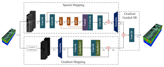
Figure 1.
Workflow of the proposed G-RDN.
In order to facilitate the discussion, we clarify the notations of some frequently used terms. The input the LR HSI and the desired HR HSI are represented as and , where w and h denote the width and height of the input LR HSI. s and n denote the scaling factor and the number of bands, respectively. denotes the super-resolved HR HSI.
2.2. Mapping between the LR HSI and the HR HSI
In the super-resolving process, the low-resolution HSI is the exclusive input, and even some prior information can be imported into the process. It still cannot be denied that the spatial information the LR HSI occupies the largest part of all the input information. In this way, the proposed method super-resolves the HSI by utilizing the spatial information in the first module. Because the bands in the HSI can be regarded as a collection of images, they were treated independently to make a full exploitation of their spatial information and gradient information and to achieve an acceptable super-resolution performance. In this way, learning the spatial mapping between the LR HSI and its HR image was the most direct way to utilize the information. In this paper, there were four parts designed in the RDN, including the shallow feature extraction (SFE) module, the local feature fusion (LFF) module, the global feature fusion (GFF) module, and the upsampling (UP) module.
Specifically, the SFE module is composed of two convolutional layers, which can be expressed by:
where is the convolutional operation and denotes the activation function achieved by the ReLU layer. is the output of the SFE module. With these shallow features obtained, they are sent into several cascaded residual dense blocks (RDBs) to extract the local features of the scene. This cascaded learning process can be expressed as:
where denotes the extraction achieved by a residual dense block. represents the output of i cascaded RDBs.
Then, the hierarchical local features extracted by each of the RDBs are merged via a concatenate layer, which can be denoted as:
where means appending the features extracted by the cascaded RDBs. is utilized to represent the output of the merged features. Meanwhile, the original input with a simple convolutional extraction is injected into the merged features to obtain the global feature, which is expressed as:
where represents the extracted feature of the original input via a shallow convolutional layer. is the output of the injection. It is noted that all the aforementioned features were extracted on the basis of the LR input HSI, whose spatial resolution was different from the desired size. In this way, an upsampling operation was applied to , and to achieve the resulting feature map with the desired size. The optimization function of this spatial mapping can be formulated as:
in which can be treated as:
2.3. Learning Gradient Mapping by the ResNet
The gradient statistics characterizes the abundance of the boundary and edge for an image, which conveys important prior information about the scene. In this paper, we imported the gradient information as the guidance for the super-resolving process via a ResNet. In order to achieve the gradient of the input HSI, both the horizontal differential kernel and the vertical differential kernel were utilized, which can be denoted as:
which is the operation occupied in the gradient-computing block in Figure 1. In this way, the gradient information of the pixel whose location is can be expressed as:
The magnitude of the gradient can be expressed as:
In Figure 2, a visual exhibition of the original Washington DC Mall and its corresponding gradient magnitude are demonstrated. As shown in Figure 2, the gradient image contains the detail information, such as the textures, the boundaries, and so on. Hence, it is rational that the gradient magnitude image can be utilized to enhance the SR performance.
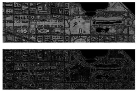
Figure 2.
Visual exhibition of the 70th band of the Washington DC Mall and its corresponding gradient magnitude.
During the learning process of the gradient, upsampling is firstly operated to obtain the gradient with the desired size:
in which is the gradient map of the input LR HSI.
Once having achieved the gradient with the desired size, a residual network with two layers is further connected to extract the features for the gradient. Meanwhile, a leaky ReLU layer acts as the activation function to represent the nonlinear mapping, which can be denoted as a function . The entire process is formulated by the expression:
For the residual network, the original upsampled gradient is injected into the output of the leaky ReLU, which can be formulated as:
In this way, the optimization function of this gradient mapping can be formulated as:
in which can be treated as:
2.4. Combination of Gradient and the Spatial Information
With the deep learning gradient and the spatial information, the final output of the G-RDN can be expressed as:
in which depicts the nonlinear mapping expressed by the G-RDN. In this way, the loss of the whole network can be formulated as follows:
in which and are the weights of the spatial information and the gradient information, respectively. The optimization of the proposed G-RDN can be expressed as:
In the experiment, the values of and were analyzed according to the performance and to determine the optimal arrangement. With the guidance of the gradient information, the super-resolving performance was improved, which will be described in detail in the following section.
3. Results
Extensive experiments were conducted to evaluate the performance of the proposed G-RDN, for which different datasets were exploited. The details of the training process and the parameter setting are introduced in this section.
3.1. Implementation Details
3.1.1. Datasets and Evaluation Metrics
We utilized three different datasets including both indoor scenes and outdoor scenes, which are described in detail as follows:
CAVE dataset: The CAVE dataset (https://www.cs.columbia.edu/CAVE/databases/multispectral, accessed on 19 May 2021) contains 32 indoor HSIs of high quality, which were obtained by a cooled CCD camera at 10 nm steps from 400–700 nm. The dataset covers a wide range of scenes including hair, food, paints, and other items. In this way, there are 31 bands for each HSI. The number of pixels is .
Pavia Center dataset: The Pavia Center dataset (http://www.ehu.eus/ccwintco/index.php/Hyperspectral_Remote_Sensing_Scenes#Pavia_Centre_and_University, accessed on 19 May 2021) was collected via the Reflective Optics System Imaging Spectrometer (ROSIS) sensor at a 1.3 m spatial resolution over Pavia, Northern Italy. There are 115 bands with a spatial size of for the scene. By removing the poor-quality area of the image and the bands with a low SNR, the size of the final HSI was .
Washington DC Mall dataset: The Washington DC Mall dataset (http://engineering.purdue.edu/~biehl/MultiSpec/hyperspectral.html, accessed on 19 May 2021) was gathered by the HYDICE sensor. There are pixels with 191 bands covering the wavelength range of 400–2400 nm. The scene contains abundant information including roof, street, grass etc.
Visual exhibitions of some typical scenes in these three datasets are demonstrated in Figure 3. All the HSIs in the CAVE dataset were captured at the ground, which makes them have comparatively finer spatial detail and a smaller scale. The other two datasets were spaceborne HSIs, and they have larger scales, but poorer spatial information, bringing a greater difficulty to the super-resolution process. By utilizing all three datasets in the experiment, the effectiveness of the proposed method on both indoor scenes with finer spatial detail and outdoor scenes with poorer spatial detail could be comprehensively evaluated, which was the same operation as described in [18,29].
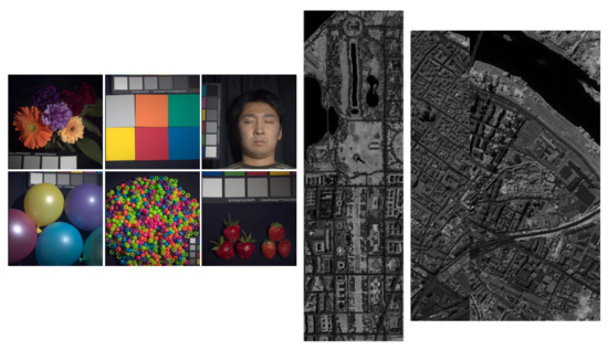
Figure 3.
Visual exhibition of some typical scenes of the three datasets utilized in this paper.
Six objective evaluation metrics were used to evaluate the effectiveness of the proposed method and the competitors. These six evaluations metrics were the root mean-squared error (RMSE), the peak-signal-to-noise ratio (PSNR), the structural similarity (SSIM), the correlation coefficient (CC), the spectral angle mapping (SAM), and the Erreur Relative Globale Adimensionnelle De Synthese (ERGAS). These six metrics can be generally classified into three categories, depending on whether they attempt to measure the spatial, spectral, or global quality of the estimated image [35]. The CC is a spatial measurement. The SAM is a spectral measurement. The RMSE, PSNR, SSIM, and ERGAS are global metrics. Specifically, among these six measurements, the RMSE, CC, PSNR, and SSIM are universal measurement matrices for image quality assessment, so their detailed descriptions were omitted in this article. The SAM evaluates the spectral preservation for all the pixels. The optimal value of the SAM is zero. The ERGAS is a global statistical measure of the SR quality whose best value is also zero. Generally speaking, the larger the CC, PSNR, and SSIM are, the better the reconstruction quality is. The RMSE, SAM, and ERGAS are exactly the opposite. To perform a comprehensive performance evaluation of the proposed G-RDN, all the datasets were downsampled by a factor of 2, 3, and 4 to achieve the LR input.
The competitors included the classical bicubic interpolation method, the pioneering SR HSI work SRCNN, and the RDN without the guidance of the gradient. Meanwhile, we also compared two fusion-based SR HSI methods, which are the NSSR [36] and the LTTR [37]. It should be noted that in order to ensure all the models shared the same input information, the auxiliary HR images required by the NSSR and LTTR were firstly averaged among all the bands, and then, an upsampling operation was applied to the average result.
3.1.2. Training Details
It is noted that for the CAVE dataset, there were 26 HSIs randomly selected as the training set, 3 HSIs were as the validation set, and the remaining 3 HSIs as the test set. Since there was only a single HSI in both Pavia Center and Washington DC Mall, spatial segmentation was utilized to achieve the three sets for the learning process. Specifically, for Pavia Center, the first 600 columns were used as the training set, and the 601st to the 665th columns were gathered as the validation set, while the remaining 50 columns acted as the test set. For the Washington DC Mall dataset, the first 1024 rows were used as the training set, the 1025th to the 1152nd rows as the validation set, and the rest 128 rows as the test set.
During the training process, the original HSI were divided into small patches whose size was , and the stride was set as one. Meanwhile, both the slide operation and the rotation operation of 90, 180, and 270 were carried to enrich the training set.
All the experiments were run on a desktop with an Intel Core i9 10850k 3.6 GHz CPU, 16 GB memory, and NVIDIA RTX 3070. The epochs for these three datasets were respectively set as 300, 200, and 200.
3.2. Parameters’ Sensitivity
In the proposed G-RDN, the gradient information of the HSI was used to constrain the SR process. Specifically, in the loss function (16), there and were set for the loss of the spatial mapping RDN and the gradient loss achieved by the ResNet, respectively.
As mentioned in Section 2.2, the spatial mapping always plays an important role in the SR process. Hence, was set to a comparatively high value during the experiment. Experimental data on the three datasets with different weight setting are demonstrated in Figure 4, at the scaling factor of two. We gradually increased the value of by a step of 0.05. It was demonstrated that when and were respectively set as 0.95 and 0.05, the performance of the G-RDN was poorer than the G-RDN with and set as 0.9 and 0.1. Meanwhile, if and were set as one and zero, the G-RDN would be the same as the RDN, whose performance was also worse than the proposed G-RDN, which will be presented in the next subsection. In addition, once the ratio of became greater, the performance of the G-RDN became worse, as demonstrated in the last three columns of Figure 4. With the growth of , the performance of the G-RDN became more worse. All the involved measure metrics including the PSNR, SSIM, and SAM exhibited the same tendency. In this way, we set and as 0.9 and 0.1 as the final weight values.
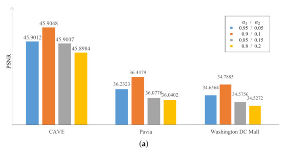
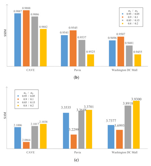
Figure 4.
Variation of the (a) PSNR, (b) SSIM, and (c) SAM with different and values.
4. Discussion
The discussion of both the objective visual comparison and the subjective measurement metrics is presented in this section.
4.1. CAVE Dataset
The HSIs in the CAVE dataset were all captured based on ground imagery sensors. The spatial information of all these HSIs is comparatively richer than that of the other two datasets. Table 1 lists the objective measurement metrics on this dataset, among which the optimal values are highlighted in bold, and the second values are also highlighted by underlines. The proposed G-RDN achieved the best value on most measurements. For the SSIM, at the scaling factor of four, our proposed G-RDN also achieved the optimal value on the PSNR, SAM, CC, RMSE, and ERGAS, and the SSIM was less than the optimal one, only 0.0001. Specifically, at the scaling factors of 2, 3, and 4, the global metric PSNR of the proposed the G-RDN achieved a 0.1 dB, 0.01 dB, and 0.04 dB improvement over the RDN, respectively. Meanwhile, it achieved nearly a 2.3 dB, 1.7 dB, and 2.7 dB improvement over the classical bicubic methods at the scaling factors of 2, 3, and 4. When it comes to the spatial metric CC, the proposed G-RDN always achieved the optimal values regardless of the scaling factor. For the spectral metric SAM, the spectral distortion brought by the proposed G-RDN was always the smallest.

Table 1.
Average measurement metrics for the three test HSIs for the CAVE dataset.
To further validate the effectiveness of the proposed G-RDN from the subjective measurement, a visual comparison of the 30th band reconstructed by different methods is demonstrated in Figure 5, Figure 6 and Figure 7, which correspond to the case with the scaling factors of 2, 3, and 4. As shown in Figure 5, the reconstructed letters in the first test HSI are clearer than those achieved by the other methods. For the second test HSI in Figure 5, the boundary of the ellipse palette reconstructed by the proposed method is sharper than those of the other methods. When it comes to the apple in the third test, it is noted that the amplified rectangle region achieved by the proposed G-RDN still owned a sharper boundary when compared with the other methods. The same phenomenon is demonstrated in Figure 6 and Figure 7. Meanwhile, for the apple region in the third test HSI in Figure 5, there were grid artifacts in the HSIs achieved by the NSSR and LTTR, which demonstrated their high dependency on the other high-resolution RGB image. It was demonstrated that rectangles reconstructed by the proposed G-RDN were always much sharper than those of the other methods. The boundary of the ellipse was also much more continuous than those reconstructed by the other methods. As for the apples in the last two rows, it is seen that the apples reconstructed by the G-RDN were closest to that in the reference image.
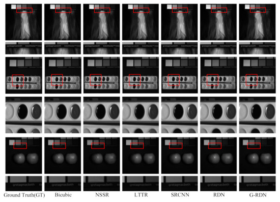
Figure 5.
Visual exhibition of the reconstructed test HSIs for the CAVE dataset at the scaling factor of 2.
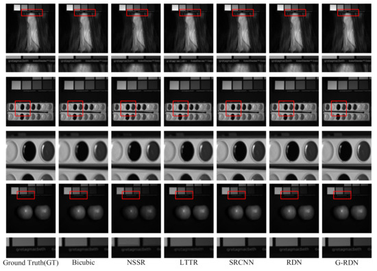
Figure 6.
Visual exhibition of the reconstructed test HSIs for the CAVE dataset at the scaling factor of 3.
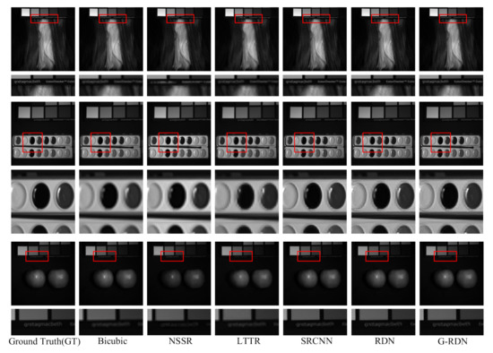
Figure 7.
Visual exhibition of the reconstructed test HSIs for the CAVE dataset at the scaling factor of 4.
To further evaluate the spectral discrimination ability of the reconstructed HSIs, we randomly selected a pixel from the reconstructed HSIs named “paints_ms” (the second scene in Figure 5) and plot the corresponding spectral curves reconstructed by different methods in Figure 8, in which Subfigure (a), (b), and (c) correspond to the scaling factors of 2, 3, and 4, respectively. It can be seen that the curve reconstructed by the proposed G-RDN was always the closest to the ground truth. Meanwhile, as the scaling factor grew, the advantage of the proposed G-RDN method was more obvious in the spectral preservation, which further proved the effectiveness of the gradient guidance.
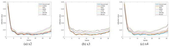
Figure 8.
Visual exhibition of the spectral curves of a randomly selected pixel in the reconstructed test HSIs.
4.2. The Pavia Center Dataset
The Pavia Center dataset covers a wider range of ground object information within a limited spatial resolution, which makes it more difficult to achieve an acceptable super-resolution performance. The objective measurements for this dataset with the scaling factors of 2, 3, and 4 are listed in Table 2. It is noted that the comparative correlation was the same as that for the CAVE dataset. All the measurements were optimal, besides the SSIM at the largest scaling factor of four. The optimal SSIM was only superior to that of the G-RDN with a gap of 0.0001, but the G-RDN outperformed it on both the PSNR and the SAM measurements. Specifically, compared with the second-best method, the CC, RMSE, and ERGAS increased by 0.0009, 0.0004, and 0.0237, respectively. Meanwhile, at the scaling factors of 2, 3, and 4, the global metric PSNR of the proposed G-RDN always achieved the optimal value. As for the metric ERGAS, it achieved a 0.026, 0.0087, and 0.0237 improvement compared with the second-best method, the RDN, when the scaling factors were 2, 3, and 4, respectively.
Table 2.
Average measurement metrics for the Pavia Center dataset.
Visualizations of the reconstructed dataset by different methods at the scaling factors of 2, 3, and 4 are displayed in Figure 9, Figure 10 and Figure 11, respectively. For the visual comparison of Pavia Center, we also selected two additional small regions with comparative rich boundary information to emphasize the spatial difference. As seen from the amplified gap in the figures, the boundaries of the gaps reconstructed by the bicubic, NSSR, and LTTR were vague, and the gap reconstructed by the proposed G-RDN was the closest to that of the ground truth. The proposed G-RDN method always restored more structural information for the roof edge in the enlarged image, and a better spatial enhancement was obtained regardless of the scaling factor.
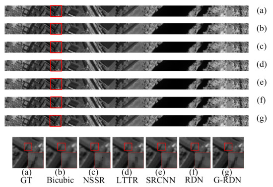
Figure 9.
Visual exhibition of the reconstructed Pavia Center at the scaling factor of 2.
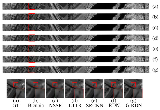
Figure 10.
Visual exhibition of the reconstructed Pavia Center at the scaling factor of 3.
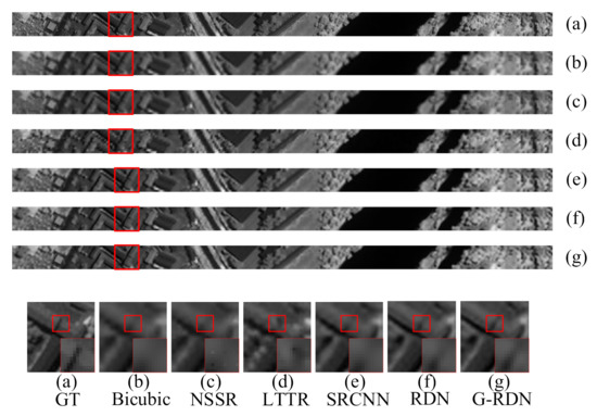
Figure 11.
Visual exhibition of the reconstructed Pavia Center at the scaling factor of 4.
In addition, to present the spectral distortion of the reconstructed image, we randomly selected one pixel from the scene and drew the corresponding spectral curves reconstructed by different methods, as shown in Figure 12. It can be clearly seen that the RDN and the G-RDN methods were obviously superior to the other methods in the spectral preservation. When compared with the RDN, the spectral curve achieved by the proposed G-RDN was closer to that of the ground truth, resulting in less spectral loss.
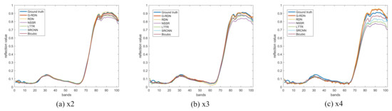
Figure 12.
Visual exhibition of the spectral curves of a randomly selected pixel in the reconstructed Pavia Center.
4.3. The Washington DC Mall Dataset
Just as Pavia Center, the Washington DC Mall dataset is also a spaceborne HSI, which had a relatively low spatial resolution when compared with the CAVE dataset. The low spatial resolution makes it more difficult in the super-resolution process. Table 3 lists the average quantitative results of different methods on the testing set from this dataset. A seen from Table 3, the proposed method still obtained the best values on both the spatial assessment metric PSNR and the spectral assessment SAM and the other metrics, except the SSIM, being superior to the other approaches and ranking first. Our SSIM was less than that of the RDN with a gap of 0.0002 when the scaling factor was three. Our PSNR achieved a 0.086 dB improvement, and the performances of the CC, RMSE, and ERGAS were improved by 0.0004, 0.0004, and 0.0844, respectively. Meanwhile, all metrics achieved the top value at the scaling factors of two and four. Specifically, the global metric PSNR of the proposed G-RDN achieved nearly 0.2 dB and 0.02 dB when the scaling factors were two and four, respectively. For the spectral metric SAM, the spectral distortion of the proposed G-RDN always achieved the best value under different scaling factors. It should be noted that the band number of Washington DC Mall was larger than that of the other two datasets. In this way, the spectral preservation was more difficult, and the SAM measurement was larger than those of the other two datasets overall.
Table 3.
Average measurement metrics for the Washington DC Mall dataset.
Figure 13, Figure 14 and Figure 15 exhibit the visualization of the reconstructed Washington DC Mall at the scaling factors of 2, 3, and 4, respectively. Seen from the amplified rectangle regions, the proposed G-RDN had advantages in restoring the structural information of the building and the surrounding details. For the reconstructed HSIs, the shape of the selected trapezoid region in the HSI achieved by the proposed method was still the clearest. When it comes to the visual figures, the shape of the selected trapezoid region was still the clearest, which further validated the effectiveness of the proposed method. Meanwhile, other competitive methods were not clear enough in the reconstruction of the edge information, and there was a visible visual gap with the proposed method. Meanwhile, to verify the spectral discrimination ability of the reconstructed HSIs, Figure 16 displays the spectral curves of a randomly selected pixel in the reconstructed HSIs, also at the scaling factors of 2, 3, and 4. The spectral curve reconstructed by the proposed method was still superior to those of the other algorithms.
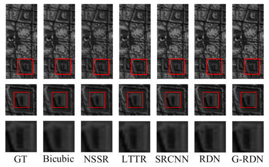
Figure 13.
Visual exhibition of the reconstructed Washington DC Mall at the scaling factor of 2.
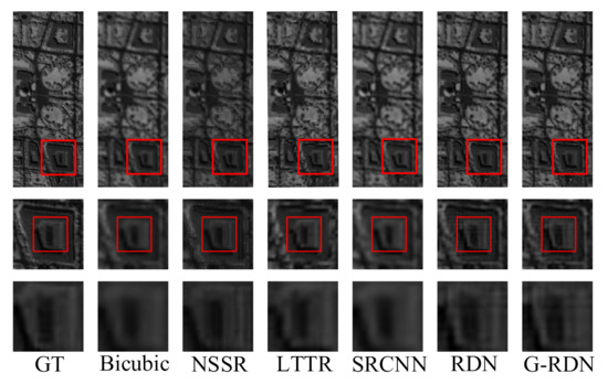
Figure 14.
Visual exhibition of the reconstructed Washington DC Mall at the scaling factor of 3.
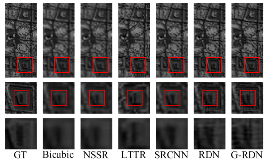
Figure 15.
Visual exhibition of the reconstructed Washington DC Mall at the scaling factor of 4.
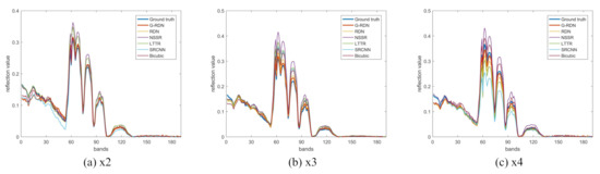
Figure 16.
Visual exhibition of the spectral curves of a randomly selected pixel in the reconstructed Washington DC Mall.
Data comparison between the RDN and the proposed G-RDN further validated the significance of the gradient guidance. Experimental results on both subjective visual effects and objective evaluation indexes verified the effectiveness of the proposed G-RDN for both ground-based HSIs and the spaceborne HSIs with poorer spatial information.
5. Conclusions
In this paper, a novel G-RDN was proposed for SR HSIs based on an end-to-end mapping between low- and high-spatial-resolution HSIs under the guidance of gradient information. Specifically, the spatial information was learned via several residual dense blocks in a hierarchical to extract the spatial feature at different levels. Meanwhile, the gradient information was learned via a ResNet and acted as a guidance for the SR process, which further improved the reconstruction performance. The spatial mapping and the gradient information were subtlety fused with an empirical weight setting. The main contribution of this paper was that, for the the first time, the gradient detail was imported to super-resolve the HSIs. Experimental results and data analysis on both the ground-based HSIs and the spaceborne HSIs with different scaling factors proved the effectiveness of the proposed G-RDN. In our future work, we will focus on how to more deeply utilize the gradient information and achieve better super-resolution performance.
Author Contributions
All of the authors made significant contributions to the manuscript. M.Z. supervised the framework design and analyzed the results. J.N. designed the research framework and wrote the manuscript. J.H. assisted in the preparation work and the formal analysis. T.L. also assisted in the formal analysis. All of the authors contributed to the editing and review of the manuscript. All authors read and agreed to the published version of the manuscript.
Funding
This work was supported by the National Natural Science Foundation of China under Grant 61901362, the Natural Science Basic Research Plan in Shaanxi Province of China under Program 2019JQ-729, the “Chunhui Plan” of the Ministry of Education of China under Grant 112-425920021, and the PhD research startup foundation of Xi’an University of Technology (Program No.112/256081809).
Institutional Review Board Statement
Not applicable.
Informed Consent Statement
Not applicable.
Data Availability Statement
The data and the details regarding the data supporting the reported results in this paper are available from the corresponding author.
Acknowledgments
The authors would like to take this opportunity to thank the Editors and the reviewers for their detailed comments and suggestions.
Conflicts of Interest
The authors declare no conflict of interest.
References
- Bioucas-Dias, J.M.; Plaza, A.; Camps-Valls, G.; Scheunders, P.; Nasrabadi, N.; Chanussot, J. Hyperspectral Remote Sensing Data Analysis and Future Challenges. IEEE Geosci. Remote Sens. Mag. 2013, 1, 6–36. [Google Scholar] [CrossRef]
- Khan, M.J.; Khan, H.S.; Yousaf, A.; Khurshid, K.; Abbas, A. Modern Trends in Hyperspectral Image Analysis: A Review. IEEE Access 2018, 6, 14118–14129. [Google Scholar] [CrossRef]
- Tratt, D.M.; Buckland, K.N.; Keim, E.R.; Johnson, P.D. Urban-industrial emissions monitoring with airborne longwave-infrared hyperspectral imaging. In Proceedings of the 2016 8th Workshop on Hyperspectral Image and Signal Processing: Evolution in Remote Sensing (WHISPERS), Los Angeles, CA, USA, 21–24 August 2016; pp. 1–5. [Google Scholar] [CrossRef]
- Yang, J.; Zhao, Y.Q.; Chan, J.C.W.; Kong, S.G. Coupled Sparse Denoising and Unmixing With Low-Rank Constraint for Hyperspectral Image. IEEE Trans. Geosci. Remote Sens. 2016, 54, 1818–1833. [Google Scholar] [CrossRef]
- Yu, H.; Shang, X.; Song, M.; Hu, J.; Jiao, T.; Guo, Q.; Zhang, B. Union of Class-Dependent Collaborative Representation Based on Maximum Margin Projection for Hyperspectral Imagery Classification. IEEE J. Sel. Top. Appl. Earth Obs. Remote Sens. 2021, 14, 553–566. [Google Scholar] [CrossRef]
- Lei, J.; Fang, S.; Xie, W.; Li, Y.; Chang, C.I. Discriminative Reconstruction for Hyperspectral Anomaly Detection with Spectral Learning. IEEE Trans. Geosci. Remote Sens. 2020, 58, 7406–7417. [Google Scholar] [CrossRef]
- Wang, Q.; Yuan, Z.; Du, Q.; Li, X. GETNET: A General End-to-End 2-D CNN Framework for Hyperspectral Image Change Detection. IEEE Trans. Geosci. Remote Sens. 2019, 57, 3–13. [Google Scholar] [CrossRef]
- Li, J.; Li, Y.; Song, R.; Mei, S.; Du, Q. Local Spectral Similarity Preserving Regularized Robust Sparse Hyperspectral Unmixing. IEEE Trans. Geosci. Remote Sens. 2019, 57, 7756–7769. [Google Scholar] [CrossRef]
- Hu, J.; Jia, X.; Li, Y.; He, G.; Zhao, M. Hyperspectral Image Super-Resolution via Intrafusion Network. IEEE Trans. Geosci. Remote Sens. 2020, 58, 7459–7471. [Google Scholar] [CrossRef]
- Li, S.; Dian, R.; Fang, L.; Bioucas-Dias, J.M. Fusing Hyperspectral and Multispectral Images via Coupled Sparse Tensor Factorization. IEEE Trans. Image Process. 2018, 27, 4118–4130. [Google Scholar] [CrossRef]
- Xu, Y.; Wu, Z.; Chanussot, J.; Wei, Z. Hyperspectral Images Super-Resolution via Learning High-Order Coupled Tensor Ring Representation. IEEE Trans. Neural Netw. Learn. Syst. 2020, 31, 4747–4760. [Google Scholar] [CrossRef] [PubMed]
- Yi, C.; Zhao, Y.Q.; Chan, C.W. Hyperspectral Image Super-Resolution Based on Spatial and Spectral Correlation Fusion. IEEE Trans. Geosci. Remote Sens. 2018, 56, 4165–4177. [Google Scholar] [CrossRef]
- Fang, L.; Zhuo, H.; Li, S. Super-Resolution of Hyperspectral Image via Superpixel-Based Sparse Representation. Neurocomputing 2017, 273, 171–177. [Google Scholar] [CrossRef]
- Fu, Y.; Zheng, Y.; Huang, H.; Sato, I.; Sato, Y. Hyperspectral Image Super-Resolution With a Mosaic RGB Image. IEEE Trans. Image Process. 2018, 27, 5539–5552. [Google Scholar] [CrossRef]
- Li, Y.; Hu, J.; Zhao, X.; Xie, W.; Li, J.J. Hyperspectral image super-resolution using deep convolutional neural network. Neurocomputing 2017, 266, 29–41. [Google Scholar] [CrossRef]
- Yuan, Y.; Zheng, X.; Lu, X. Hyperspectral Image Superresolution by Transfer Learning. IEEE J. Sel. Top. Appl. Earth Obs. Remote Sens. 2017, 10, 1963–1974. [Google Scholar] [CrossRef]
- Xie, W.; Jia, X.; Li, Y.; Lei, J. Hyperspectral Image Super-Resolution Using Deep Feature Matrix Factorization. IEEE Trans. Geosci. Remote Sens. 2019, 57, 6055–6067. [Google Scholar] [CrossRef]
- Mei, S.; Yuan, X.; Ji, J.; Zhang, Y.; Wan, S.; Du, Q. Hyperspectral Image Spatial Super-Resolution via 3D Full Convolutional Neural Network. Remote Sens. 2017, 9, 1139. [Google Scholar] [CrossRef]
- Li, Q.; Wang, Q.; Li, X. Mixed 2D/3D Convolutional Network for Hyperspectral Image Super-Resolution. Remote Sens. 2020, 12, 1660. [Google Scholar] [CrossRef]
- Xu, X.; Zhong, Y.; Zhang, L.; Zhang, H. Sub-Pixel Mapping Based on a MAP Model With Multiple Shifted Hyperspectral Imagery. IEEE J. Sel. Top. Appl. Earth Obs. Remote Sens. 2013, 6, 580–593. [Google Scholar] [CrossRef]
- Wang, X.; Ma, J.; Jiang, J. Hyperspectral Image Super-Resolution via Recurrent Feedback Embedding and Spatial-Spectral Consistency Regularization. IEEE Trans. Geosci. Remote Sens. 2021, 1–13. [Google Scholar] [CrossRef]
- Mei, S.; Jiang, R.; Li, X.; Du, Q. Spatial and Spectral Joint Super-Resolution Using Convolutional Neural Network. IEEE Trans. Geosci. Remote Sens. 2020, 58, 4590–4603. [Google Scholar] [CrossRef]
- Liu, D.; Li, J.; Yuan, Q. A Spectral Grouping and Attention-Driven Residual Dense Network for Hyperspectral Image Super-Resolution. IEEE Trans. Geosci. Remote Sens. 2021, 1–15. [Google Scholar] [CrossRef]
- Wang, Q.; Li, Q.; Li, X. Hyperspectral Image Super-Resolution Using Spectrum and Feature Context. IEEE Trans. Ind. Electron. 2020. [Google Scholar] [CrossRef]
- Dong, C.; Loy, C.C.; He, K.; Tang, X. Image Super-Resolution Using Deep Convolutional Networks. IEEE Trans. Pattern Anal. Mach. Intell. 2016, 38, 295–307. [Google Scholar] [CrossRef] [PubMed]
- Jia, J.; Ji, L.; Zhao, Y.; Geng, X. Hyperspectral image super-resolution with spectral–spatial network. Int. J. Remote Sens. 2018, 39, 7806–7829. [Google Scholar] [CrossRef]
- Yokoya, N.; Yairi, T.; Iwasaki, A. Coupled Nonnegative Matrix Factorization Unmixing for Hyperspectral and Multispectral Data Fusion. IEEE Trans. Geosci. Remote Sens. 2012, 50, 528–537. [Google Scholar] [CrossRef]
- Wang, Q.; Li, Q.; Li, X. Spatial-Spectral Residual Network for Hyperspectral Image Super-Resolution. arXiv 2020, arXiv:2001.04609. [Google Scholar]
- Li, Q.; Wang, Q.; Li, X. Exploring the Relationship Between 2D/3D Convolution for Hyperspectral Image Super-Resolution. IEEE Trans. Geosci. Remote Sens. 2021, 1–11. [Google Scholar] [CrossRef]
- Ledig, C.; Theis, L.; Huszar, F.; Caballero, J.; Cunningham, A.; Acosta, A.; Aitken, A.; Tejani, A.; Totz, J.; Wang, Z. Photo-Realistic Single Image Super-Resolution Using a Generative Adversarial Network. IEEE Comput. Soc. 2016. [Google Scholar]
- Kim, J.; Lee, J.K.; Lee, K.M. Accurate Image Super-Resolution Using Very Deep Convolutional Networks. In Proceedings of the 2016 IEEE Conference on Computer Vision and Pattern Recognition (CVPR), Las Vegas, NV, USA, 27–30 June 2016; pp. 1646–1654. [Google Scholar] [CrossRef]
- Lim, B.; Son, S.; Kim, H.; Nah, S.; Lee, K.M. Enhanced Deep Residual Networks for Single Image Super-Resolution. In Proceedings of the 2017 IEEE Conference on Computer Vision and Pattern Recognition Workshops (CVPRW), Honolulu, HI, USA, 21–26 July 2017. [Google Scholar]
- Tong, T.; Li, G.; Liu, X.; Gao, Q. Image Super-Resolution Using Dense Skip Connections. In Proceedings of the IEEE International Conference on Computer Vision, Venice, Italy, 22–29 October 2017. [Google Scholar]
- Zhang, Y.; Tian, Y.; Kong, Y.; Zhong, B.; Fu, Y. Residual Dense Network for Image Super-Resolution. In Proceedings of the 2018 IEEE/CVF Conference on Computer Vision and Pattern Recognition, Salt Lake City, UT, USA, 18–22 June 2018. [Google Scholar]
- Loncan, L.; de Almeida, L.B.; Bioucas-Dias, J.M.; Briottet, X.; Chanussot, J.; Dobigeon, N.; Fabre, S.; Liao, W.; Licciardi, G.A.; Simões, M.; et al. Hyperspectral Pansharpening: A Review. IEEE Geosci. Remote Sens. Mag. 2015, 3, 27–46. [Google Scholar] [CrossRef]
- Dong, W.; Fu, F.; Shi, G.; Cao, X.; Wu, J.; Li, G.; Li, X. Hyperspectral Image Super-Resolution via Non-Negative Structured Sparse Representation. IEEE Trans. Image Process. 2016, 25, 2337–2352. [Google Scholar] [CrossRef]
- Dian, R.; Li, S.; Fang, L. Learning a Low Tensor-Train Rank Representation for Hyperspectral Image Super-Resolution. IEEE Trans. Neural Netw. Learn. Syst. 2019, 30, 2672–2683. [Google Scholar] [CrossRef]


Publisher’s Note: MDPI stays neutral with regard to jurisdictional claims in published maps and institutional affiliations. |
© 2021 by the authors. Licensee MDPI, Basel, Switzerland. This article is an open access article distributed under the terms and conditions of the Creative Commons Attribution (CC BY) license (https://creativecommons.org/licenses/by/4.0/).