Article

Studying the Feasibility of Assimilating Sentinel-2 and PlanetScope Imagery into the SAFY Crop Model to Predict Within-Field Wheat Yield

1
Agricultural Research Organization, Volcani Institute, Institute of Soil, Water and Environmental Sciences, HaMaccabim Road 68, P.O. Box 15159, Rishon LeZion 7528809, Israel
2
Amrita School of Agricultural Sciences, Amrita Vishwa Vidyapeetham, J. P. Nagar, Arasampalayam, Myleripalayam, Coimbatore 642 109, Tamil Nadu, India
3
School of Earth, Atmosphere and Environment, Monash University, Clayton, VIC 3800, Australia
4
Field Crops and Natural Resources Department, Agricultural Research Organization, Gilat Research Center, M.P. Negev 8531100, Israel
*
Author to whom correspondence should be addressed.
Remote Sens. 2021, 13(12), 2395; https://doi.org/10.3390/rs13122395
Submission received: 19 April 2021 / Revised: 9 June 2021 / Accepted: 15 June 2021 / Published: 19 June 2021

Abstract

:
Spatial information embedded in a crop model can improve yield prediction. Leaf area index (LAI) is a well-known crop variable often estimated from remote-sensing data and used as an input into crop models. In this study, we evaluated the assimilation of LAI derived from high-resolution (both spatial and temporal) satellite imagery into a mechanistic crop model, a simple algorithm for yield estimate (SAFY), to assess the within-field crop yield. We tested this approach on spring wheat grown in Israel. Empirical LAI models were derived from the biophysical processor for Sentinel-2 LAI and spectral vegetation indices from Sentinel-2 and PlanetScope images. The predicted grain yield obtained from the SAFY model was compared against the harvester’s yield map. LAI derived from PlanetScope and Sentinel-2 fused images achieved higher yield prediction (RMSE = 69 g/m2) accuracy than that of Sentinel-2 LAI (RMSE = 88 g/m2). Even though the spatial yield estimation was only moderately correlated to the ground truth (R2 = 0.45), this is consistent with current studies in this field, and the potential to capture within-field yield variations using high-resolution imagery has been demonstrated. Accordingly, this is the first application of PlanetScope and Sentinel-2 images conjointly used to obtain a high-density time series of LAI information to model within-field yield variability.

1. Introduction

A priori knowledge of crop yield is useful for stakeholders along the value chain and policymakers in their decision-making process [1]. Early studies on crop yield prediction used climate variables (e.g., precipitation, air temperature, solar radiation) to develop empirical models using historical crop yield data. However, these empirical relationships between crop yield and climate variables vary from region to region. Thus, the models are not general enough, and their applicability to new regions is limited [2,3]. The technological advancement in sensors, computational tools, and remote sensing science provide a vast volume of digital data to monitor and assess the spatial variability of crop yield [4]. For instance, earth observation satellites monitor land cover changes at short intervals [5]. Spectral vegetation indices derived from satellite images were found to be well correlated with crop variables, including leaf area index (LAI) and yield [6,7,8]. However, many traditional vegetation indices (VI) suffer from saturation, i.e., VI values remain almost the same at higher LAI values (LAI >3) in dense crop canopies [6,7]. In addition, yield estimations based on spectral vegetation indices alone do not account for other yield-contributing factors, namely crop management operations (e.g., irrigation, fertilization), variability in weather, and soil types [8,9].
Mechanistic crop models consist of a set of equations that model crop physiological processes to predict crop yield. Crop models simulate the complex interaction of crop growth with varying soil, water, and climatic conditions. Moreover, these models have been applied to a wide range of growing conditions across the globe [10]. However, crop models simulate a unit area for which the conditions are assumed homogeneous. Because of this assumption, within-field spatial variability of soil conditions and management operations is often disregarded. However, satellite images can capture this variability in the field when it affects crop growth, and when coupled with crop models, they introduce a spatial component to the models. Previous attempts to embed such information from earth observation into crop models included estimations of the fraction of absorbed photosynthetically active radiation, LAI, canopy cover, biomass, soil moisture, and evapotranspiration [11].
LAI is one of the most commonly used variables in agronomic crop models that can be estimated from remote-sensing imagery [3,12,13,14]. Previously, LAI data from an external source has been assimilated into various crop models, namely DSSAT, WOFOST, and STICS, to improve yield predictions [13,15,16,17,18,19]. However, some crop models are complicated to run since they require many input parameters and variables. Among various crop models, the Simple Algorithm For Yield estimate (SAFY) [20] requires few inputs (including from remote-sensing) for operational yield prediction. Since SAFY does not have a water and nutrient component, the model assumes that the stress-induced growth reduction affects the LAI values and ultimately determines the yield. The SAFY model has been validated for wheat [21,22,23,24,25] and maize [26,27] under different climatic conditions. Moreover, vegetation indices derived from satellite imagery were found to be related quasi-linearly (enhanced vegetation index; EVI) or non-linearly (normalized difference vegetation index; NDVI) to LAI [28]. Thus, using information from spaceborne sensors or proximal sensing to update growth information in a crop model is a promising approach to improving yield predictions while considering spatial crop heterogeneity [8,29].
The growing number of satellite observations at finer spatial resolution facilitates continuous crop monitoring and yield prediction at the field and subfield scales. However, until recently, this approach was stalled by the lack of satellite images at an adequate revisiting time with a high spatial resolution [30]. Nowadays, high-quality public domain earth observation data such as Landsat-8 and Sentinel-2 are widely available. Moreover, a new generation of nano-satellites, such as Planet Labs’ PlanetScope CubeSat constellation, provides cost-effective high spatial and temporal resolution images [31,32]. However, PlanetScope images tend to suffer from cross-sensor inconsistencies that introduce noise to the time series of observations acquired from these sensors [33,34]. This cross-sensor noise hinders the use of PlanetScope for precise crop monitoring applications [31]. To overcome this limitation, the fusion of PlanetScope images with a consistent and reliable dataset, such as Sentinel-2, can eliminate the noise in PlanetScope data [35]. Additionally, this fusion can be used to create a high spatio-temporal dataset that benefits from the short revisit time and high spatial resolution of PlanetScope, together with the radiometric consistency of Sentinel-2.
Previously, a few studies explored the use of satellite images to study yield variability. These field-scale studies used high-resolution public domain images [36], commercial satellite images [37], and a combination of images from different sensors [38]. Recent studies produced empirical models at both field/plot and sub-plot levels between crop yield and vegetation indices derived from satellite images, namely Sentinel-2 [36,39,40,41,42], Landsat 8 [40,41], and HJ-CCD images [43]. Furthermore, it would be interesting to explore the assimilation of high-resolution satellite imagery such as PlanetScope images from spaceborne sensors into mechanistic crop models for within-field yield variability estimations [44]. The potential of high-resolution images such as Sentinel-2 and PlanetScope to estimate the yield at field scale was previously explored in a few studies [27,45,46]. Thus, assessing the accuracies of the public domain (Sentinel-2) as well as commercial (PlanetScope) satellite data to study the within-field yield production is a hot topic since these open data sources can be used for low-cost yield forecasting [36].
The overarching aim of this research was to improve yield prediction by integrating high-resolution satellite imagery into the SAFY crop model. Since ongoing earth observation missions (e.g., PlanetScope and Sentinel-2) can produce a time series of spectral vegetation indices, LAI estimations can be derived based on these indices and integrated into the SAFY model to replace the model’s own LAI state variable. This enables to model each pixel (i.e., within-field regions) to study the yield variation. Subsequently, the usefulness of incorporating high spatial and temporal resolution data from Sentinel-2 and PlanetScope images into the mechanistic crop model SAFY was tested to improve within-field wheat yield prediction. The specific objectives of the study were to (1) test the impact of different LAI estimation models from remote sensing data on the yield estimation; (2) explore the impact of spatial and temporal resolution on yield prediction.

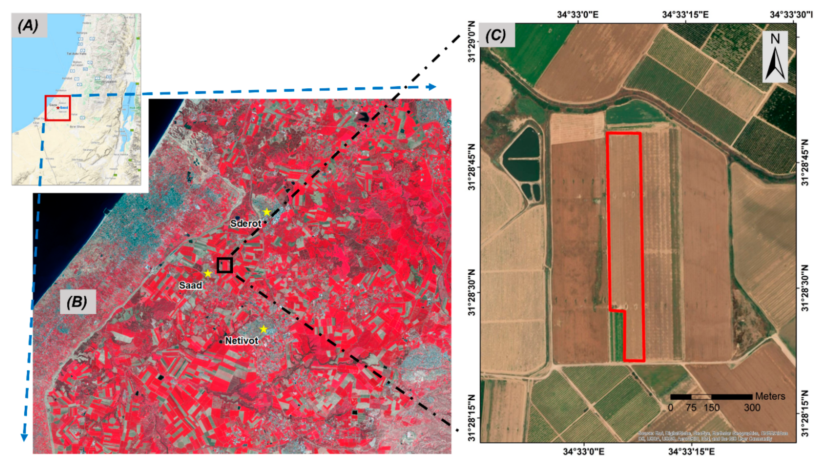
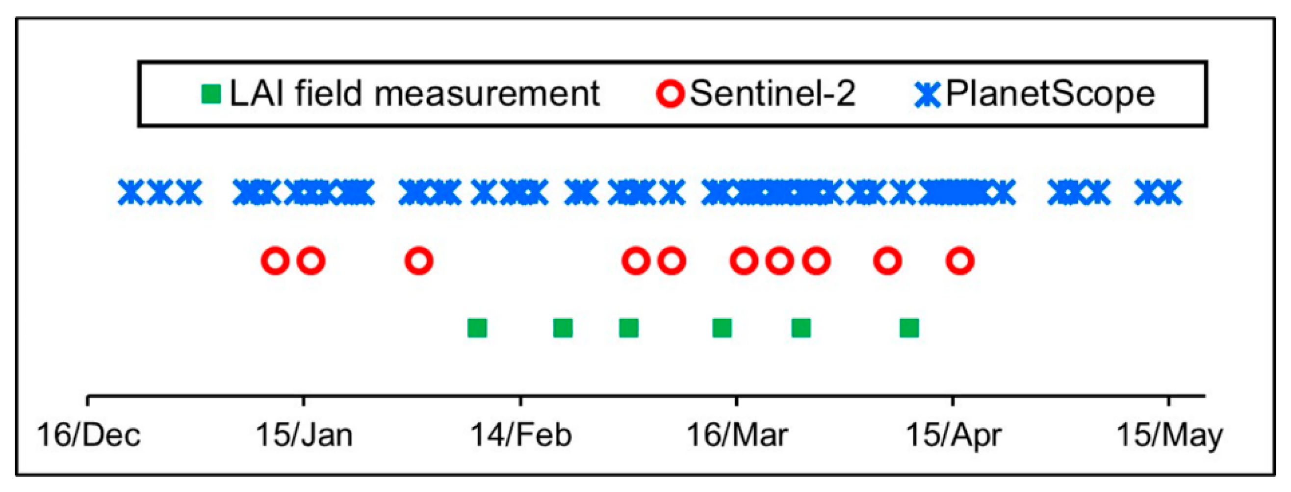
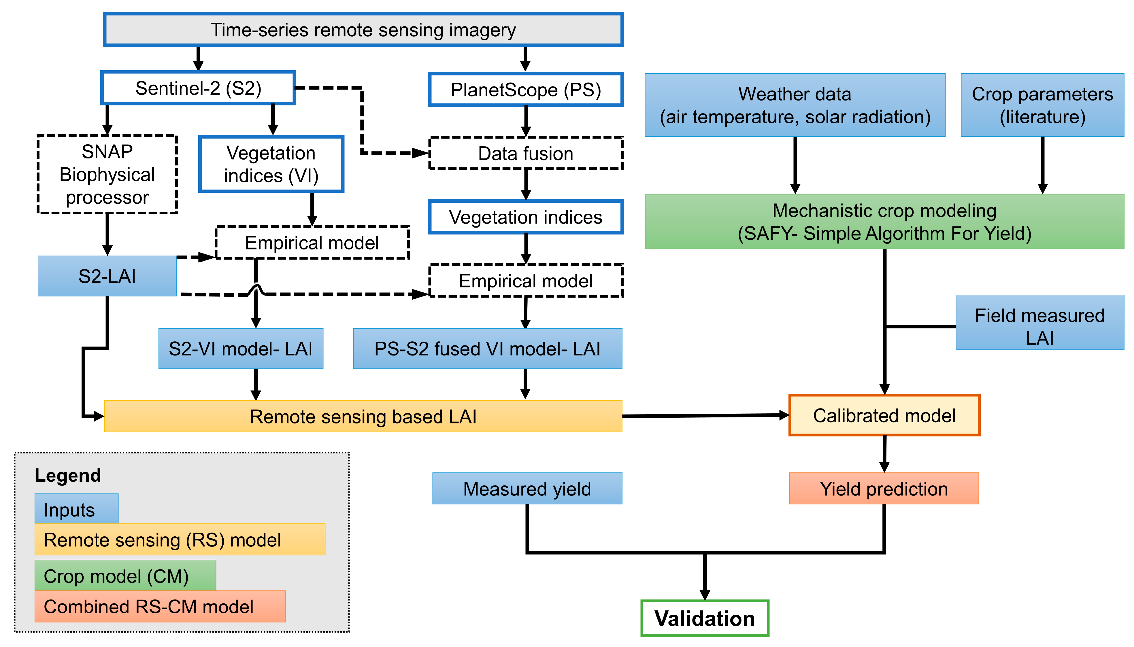
2. Materials and Methods

A commercial wheat field covering an area of 52,000 m2 near Saad in Israel was chosen for this study (Figure 1). Spring wheat (cv. Amit) was cultivated as a rainfed winter crop, sown on 22 December 2017, and harvested on 23 May 2018. LAI values were measured using the SunScan Canopy Analysis System (SS1 developed by Delta-T Company, Cambridge, United Kingdom) [47]. A time series of cloud-free Sentinel-2 (S2) and PlanetScope (PS) images were acquired throughout the wheat growing season (Figure 2). Sentinel-2 data were downloaded from the European Space Agency’s Copernicus Open Access Hub website (https://scihub.copernicus.eu/dhus/#/home, accessed on 19 April 2021). The cloud-free PlanetScope images were downloaded using Planet’s API (https://api.planet.com, accessed on 19 April 2021). Level-2 atmospherically corrected Sentinel-2 and PlanetScope surface reflectance products were used in the analysis [48].

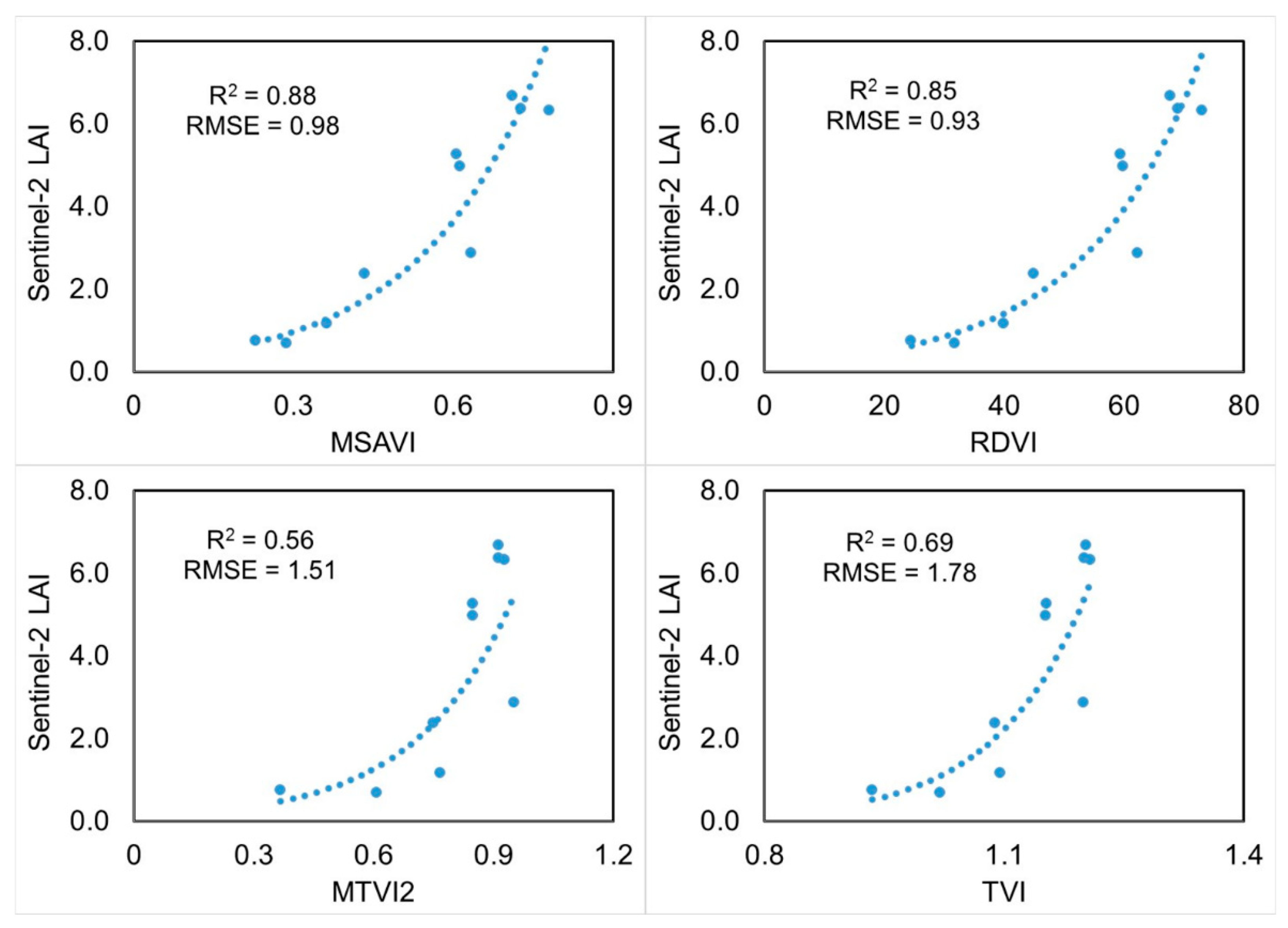
2.1. LAI Maps Creation

First, the Biophysical Processor module [49] embedded in the SentiNel Application Platform (SNAP) [50] was used to derive LAI estimations from Sentinel-2 Level-2A Bottom of Atmosphere (BOA) reflectance. This processor uses top-of-canopy reflectance data to estimate a number of biophysical variables, including LAI. These estimations will henceforward be referred to as S2-LAI images. PlanetScope (55 images) and Sentinel-2 (10 images) images were fused to obtain high spatial and temporal resolution images following the work of Sadeh et al. [35]. These fused images were used to derive 13 vegetation indices (Table A1) from which high-resolution LAI images were created. Further, this spatial LAI dataset was compared against field-measured LAI and the indices that showed the best LAI estimations for wheat, namely, MTVI2, MSAVI, RDVI, and TVI [35]. In addition, empirical functions were also derived between the spectral indices from Sentinel-2 images and the S2-LAI. All three remote-sensing-based LAI maps were used as an external spatial input into a crop model (Figure 3).
Ten cloud-free Sentinel-2 images (Figure 2) covering the entire wheat-growing season were used for deriving the S2-LAI product (biophysical processor). The empirical relationship between the S2-LAI and spectral indices based on Sentinel-2 and PlanetScope images was derived.

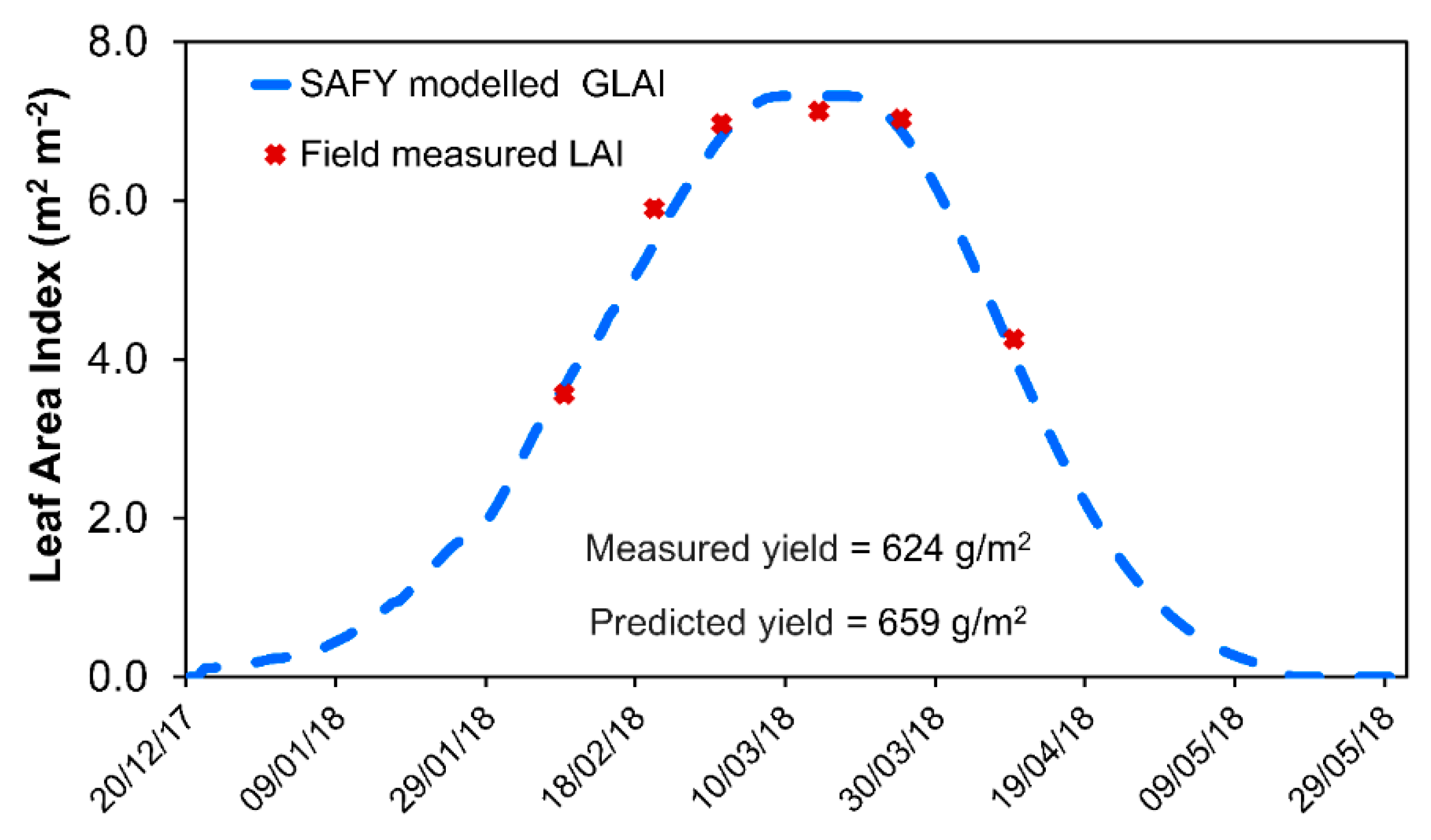
2.2. Simple Algorithm for Yield Estimate (SAFY) Model

The SAFY crop model was employed to simulate the basic biophysical processes of leaf growth and senescence using semi-empirical functions [20]. The SAFY model calculates the increase in dry, above-ground biomass by accounting for the influence of temperature and the dynamics of green leaves (Figure 4). SAFY requires weather and crop variables as inputs. The air temperature and solar irradiance were available from the agricultural meteorology unit of the Israel Ministry of Agriculture and Rural Development at http://www.meteo.co.il/, accessed on 19 April 2021 (temperature and solar radiation data from Dorot and Mavkiim stations, respectively). Most of the crop parameters (Table 1) for SAFY were available in the literature, obtained through remote-sensing data, or otherwise optimized through calibration [20,22,23].
ΔDAM = Rg × εC × εI × ELUE × FT(Ta)
εI = 1 − e(−k × GLAI)
where DAM = dry above-ground mass (g m−2), Rg = daily incoming global radiation (MJ m−2 d−1), εC = climatic efficiency (unitless), εI = light-interception efficiency (a function of leaf area index and a light-interception coefficient) (g MJ−1), ELUE = effective light-use efficiency (the ratio of photochemical energy produced as DAM from APAR) (unitless), Ta = daily mean air temperature (°C), k = light-interception coefficient (unitless), and GLAI = green leaf area index (m2 m−2).
The MATLAB version of SAFY [20] was modified to receive LAI externally from earth observation data (Figure 4). The external LAI is the product of a time series of spectral vegetation indices from Sentinel-2 and PlanetScope images; LAI estimations can be derived based on these indices. Prior to LAI integration, an initial model simulation was performed to calibrate the model to the field conditions: The default wheat parameter dataset (provided with the original SAFY version) was used as the starting basis to establish a modified parameter set for wheat yield simulation. Planting and harvesting dates were collected from the field. Wheat parameters were modified using values from the literature to account for the local context. Crop parameters were calibrated by comparing the SAFY-modeled LAI with in-situ values of field-measured LAI [25]. The parameters were optimized to receive the lowest root mean square error (RMSE) between field-measured LAI and the SAFY-modeled LAI values (Figure 5), as well as SAFY-modeled yield, which was as close as possible to the average observed yield. The final crop parameters are listed in Table 1. A pixel-wise model simulation was carried out using satellite images as an external input in the calibrated SAFY model (Figure 4).
The LAI values derived from the S2, PS, and S2 fused images were used as an input into the SAFY model in this study. LAI maps were generated from these daily vegetation indices. The time series of LAI data were smoothed using a quadratic polynomial Savitzky–Golay filter to reduce the noise [51]. The smoothed LAI at the pixel level was linearly interpolated to fill the gaps daily and then assimilated using a forcing strategy to replace the SAFY model LAI (Figure 3).
Yield prediction using SAFY was performed for every pixel in the field. Several different remote-sensing based LAI estimations were used for yield prediction, namely (i) S2-LAI; (ii) LAI derived from Sentinel-2 MSAVI and S2-LAI model; (iii) LAI derived from Sentinel-2 MSAVI and field-measured LAI, and (iv) LAI derived from fused PS-S2 MSAVI and S2-LAI model. Further, we tested three scenarios to study the impact of spatial and temporal resolution, i.e., (i) reduced revisit time, (ii) reduced revisit time and spatial resolution, and (iii) reduced spatial resolution.

2.3. Pre-Processing of Yield Monitor Data
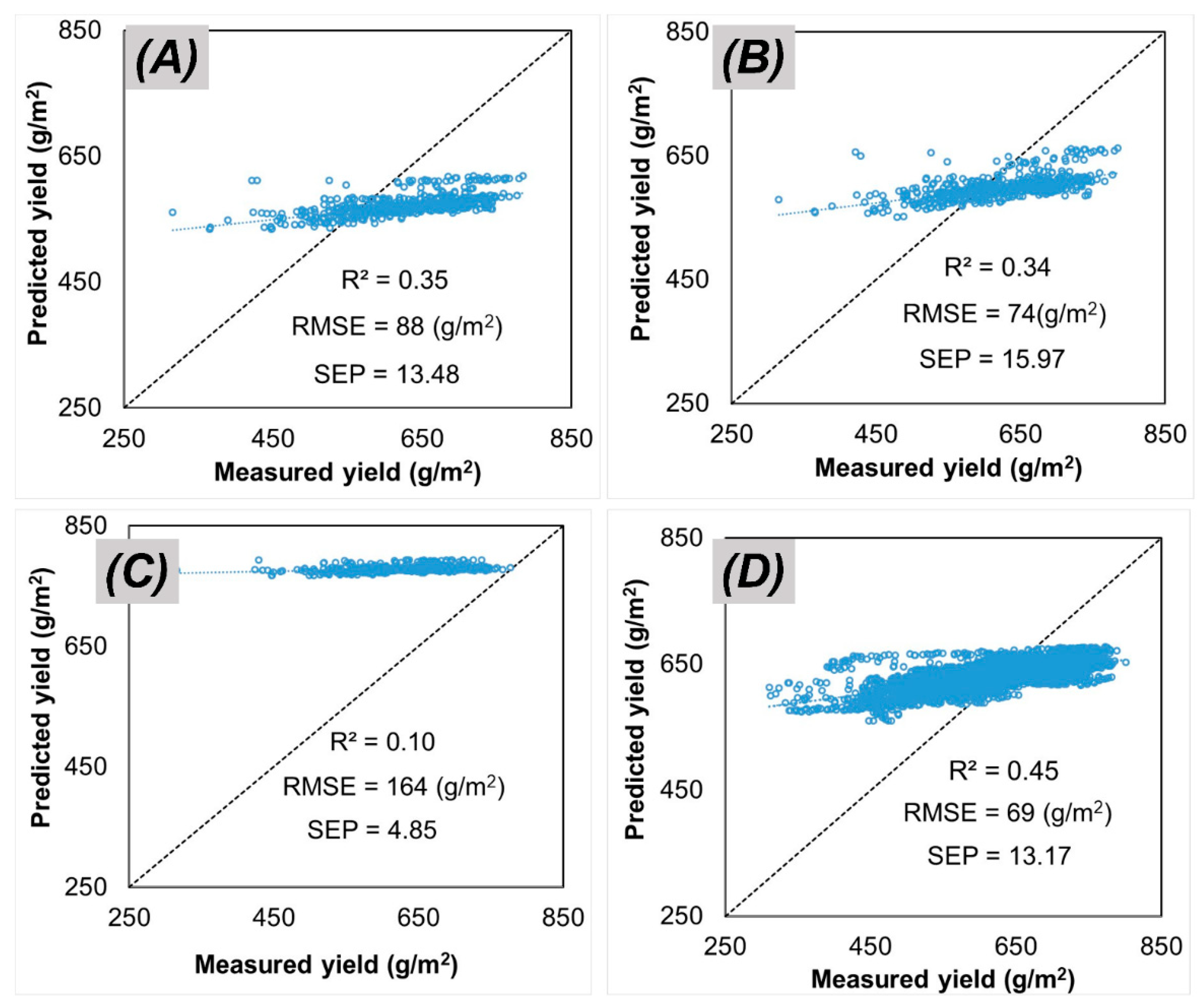
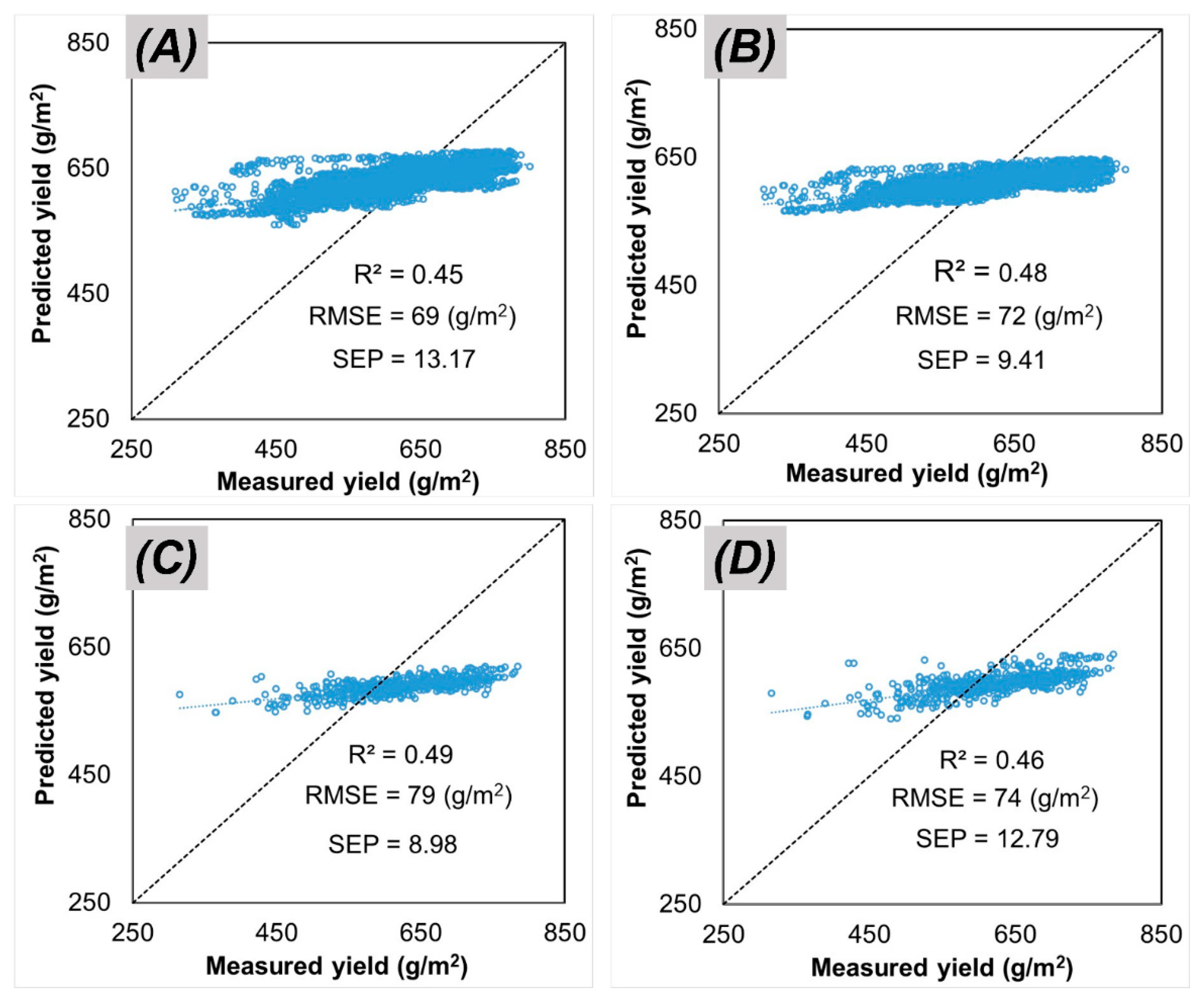
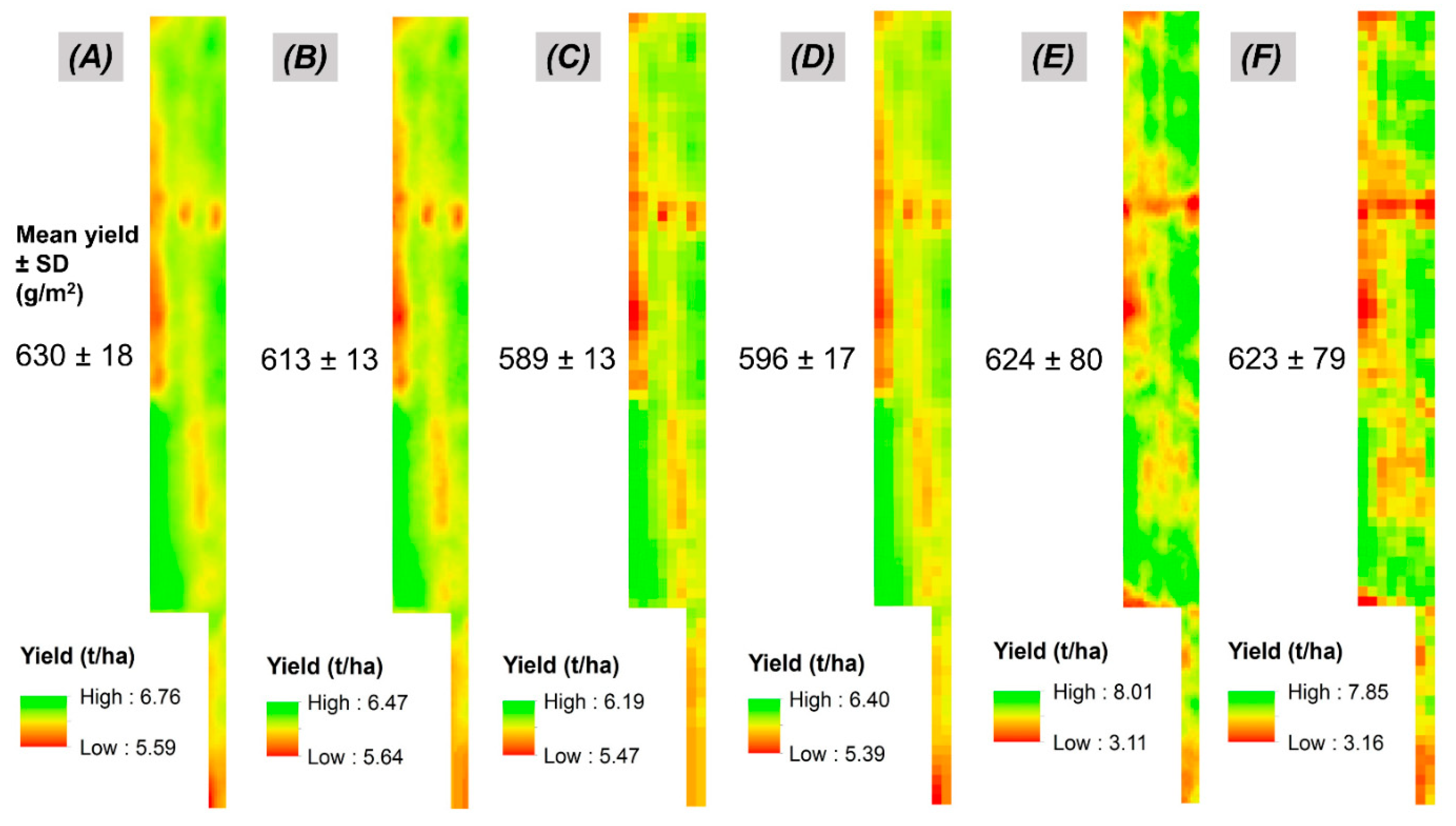
SAFY yield estimates were compared against the measured grain yield obtained from a harvester equipped with a yield monitoring system that records the grain yield at high spatial resolution. This yield data was used to assess the potential of fine-resolution images to estimate crop yield [36,42]. First, the yield point map was pre-processed: Yield points of less than 0.1 t ha−1 were omitted, a buffer of 10 m from the edge was ignored to avoid edge effects, and, in addition, yield values larger than mean ± three standard deviations were excluded as outliers [52,53]. Next, ordinary kriging interpolation was performed to generate the final yield map. The yield data points were interpolated to the standard grid of 3 × 3 m and 10 × 10 m, coincident with PlanetScope and Sentinel-2 images. In this study, LAI derived from satellite images was the sole input for the crop model other than weather data. The field-measured LAI was used for SAFY model calibration and to derive an empirical relation with Sentinel-2 MSAVI.

3. Results

Out of four indices that were found to best estimate LAI in Sadeh et al. [35], MSAVI showed the strongest correlation with S2-LAI (R2 = 0.88, RMSE = 0.98), followed by RDVI (R2 = 0.85, RMSE = 0.93) (Figure 6). Since MSAVI showed better prediction performance, subsequent results are based on MSAVI-based LAI.
Among four LAI models, PS-S2 fused images showed better yield estimation compared to S2, owing to the high spatial and temporal resolution (PS-S2 fused images) (Figure 7d). The predicted average yield (572–630 g/m2) showed acceptable bias from the observed yield (624 g/m2). Even though the predicted yield showed a narrower range of variation than the observed yield, the observed yield’s spatial pattern was well captured in the predicted yield maps (Figure 8).
Deviations between simulated and observed yield occurred mainly when the model predicted higher yields (Figure 7). These higher predicted yields correspond to the lower-left corner of the image (Figure 8A–D) that failed to capture the observed yield (Figure 8E). The superior spatial resolution of the PS images the small details shown in the yield prediction map (Figure 8D).
The impact of spatial and temporal resolution on yield prediction was explored using three different scenarios, as shown in Figure 9B–D. The prediction error (RMSE) was found to be sensitive to the revisit time when the high PS spatial resolution was retained (Figure 9A), and the error increased as the spatial and temporal resolutions were reduced to those of S2 (Figure 9B–D). Resampling to lower resolution (both spatial and temporal; Figure 10B–D) increased average crop yield bias. However, the low-resolution images (both spatial and temporal; Figure 10D) still captured the spatial pattern very well. Thus, PlanetScope and Sentinel-2 images are capable of capturing the dynamics of crop growth.

4. Discussion

Crop models mostly adopt the LAI-based radiation use efficiency approach to simulate crop biomass since the rate of LAI changes shows crop growth development. In addition, many studies have attempted to assimilate remotely sensed LAI into crop models [11]. This research found that the LAI maps derived from high-resolution images are good for continuous updates during crop development. High spatial resolution images deliver more accurate details of the spatial variations. Similarly, a sufficient number of images with good temporal distribution throughout the growing season is desired in order to capture crop growth well [54]. PlanetScope images offer higher spatial and temporal information that facilitates monitoring within-field variation [55]. This is the first study, to our knowledge, to use PlanetScope images in wheat yield modeling. In addition, the ongoing earth observation missions, Sentinel-2 and Landsat-8, as well as their cross-sensor harmonized products, provide a potential source for continuous observations throughout the crop-growing season [56,57].
The range of observed grain yield was between 311 and 801 g/m2, while the estimated yield range was between 533 and 793 g/m2 (Figure 8). Therefore the model did not well capture the range of variability in the observed yield. Figure 11 explains this failure: The changes in final biomass are quite low, even after a 50% reduction in LAI (due to the LAI and DAM relationship; Equation (2)). Thus, the model failed to predict low- and high-yield values. Certain modifications to the SAFY model are required to improve the within-field yield prediction. For example, the LUE parameter used in the SAFY model (Equation (1)) can vary within-field depending on factors such as temperature, the nitrogen concentration in leaves, and water availability to the crop. Instead of using LUE as a constant (i.e., ELUE; Table 1), LUE’s spatial distribution can be included as a function, which serves as a yield-limiting factor to capture the within-field variability [44]. Furthermore, factors such as LAI saturation in wheat, mixed pixels, and other biotic and abiotic stress effects on crop yield that are not accounted for in the model may contribute to underperformance of model prediction on the low- and high-yield values [9].
The yield estimation was only moderately correlated to the ground truth in this study (R2 = 0.45). A recent study from Deines et al. [58] also highlighted that the prediction accuracy is moderate at the pixel level (R2 = 0.40) compared to the county scale (R2 = 0.69) and field-level (R2 = 0.45), even after using fine-scale yield monitor data for model calibration. Although the SAFY model failed to capture the within-field variability, this study’s prediction error showed better performance compared to previous studies that used the same model for wheat yield prediction (Table 2). Although this simple model does not consider factors such as water and nutrient-induced stress, the dynamics of green leaves (times series of LAI) seems to account for much of the external stress [20].
This study demonstrated for the first time that PlanetScope and Sentinel-2 provide high-resolution dense time-series information from which the crop variable (LAI) can be derived and embedded in the SAFY model to produce a within-field yield variability map. These types of studies can be useful for web-based services in the future. Since both the satellite imagery and the crop models come at no cost, a Google Earth Engine-based web application has the potential to serve as a low-cost crop yield monitoring tool for growers’ farm management operations and policymakers at the government level [8]. Another advantage of this simplified approach is the ease of implementation of new regions. Further, a validated model can be used to predict the in-season as well as final crop yield using real-time satellite images along with weather forecast data.
This study used high-resolution yield data for validation. However, the yield monitor data were not perfect ground truth but rather were pre-processed to exclude some of the significant errors; not all bias was removed, which affected the validation. Specifically, the remaining bias increased the deviation between observed and predicted yield since the high-resolution image pixels were insufficient to discern small features in the field. The within-field variability analysis can benefit growers by facilitating site-specific farm management operations [60]. Further, developing the spatial variability yield model at the sub-plot level remains challenging due to the following reasons: (i) a lack of high-resolution yield information at a sufficient scale, (ii) affordability and accessibility of digital data at the sub-plot level, (iii) a lack of a comprehensive crop monitoring system to coordinate and access the various field dataset in real-time [32].
Similar to previous studies [11], this study showed that spatial LAI is an effective input to crop models. However, our results (Figure 11) showed that SAFY must be improved, e.g., by developing a LUE function, to successfully model within-field variability. Similarly, spatial modeling at the sub-plot level should be tested with other crop models in future studies.
Overall, combining the high-resolution PS-S2 LAI products with the SAFY model is easy, owing to their simplicity. However, the poor performance of the SAFY model, demonstrated by the low R2, could be attributed to multiple factors such as (i) LAI in the SAFY model was replaced by a time-series of S2/PS LAI product that represents the dynamics of green leaves, and thus accounting for the field conditions (e.g., stress) at each pixel. However, uncertainties related to LAI estimation from satellite images necessitates further examination in future studies; (ii) The compatibility of SAFY to various spatial scales requires further investigation as the model may not adequately describe important processes at some spatial scales (e.g., SAFY does not account for nutrient variability content at a higher resolution [44]); (iii) Additional studies can perform a sensitivity analysis to identify the most influencing SAFY model parameters on yield prediction; (iv) We used the forcing method, i.e., direct replacement approach to integrating S2/PS LAI products into the SAFY model. Future studies could examine well-known data assimilation algorithms such as Ensemble Kalman Filter (EnKF) and Four-Dimensional Variational Data Assimilation (4DVAR) to reduce the bias between remote sensing observation and simulated values.

5. Conclusions

This study showed the potential of current high-resolution earth observation satellite missions to create dense time-series of crop variables (LAI) and predict the yield at high resolution. We tested four different LAI models as an external input to the SAFY model to predict wheat yield. Among all, LAI derived from PS-S2 fused images showed higher accuracy for yield estimation than did S2 images alone (RMSE = 69 and 88 g/m2, respectively). Three scenarios were employed to study the impact of spatial and temporal resolution. Both PlanetScope and Sentinel-2 can capture the spatial pattern well. The high-resolution PS-S2 fused images showed a very low average crop yield bias (6 g/m2) compared to low-resolution S2 images (34 g/m2).
Conversely, the high-resolution images showed a moderate correlation (R2 = 0.45) with the within-field variability. Lower values of R2 could result from factors such as operational error from yield monitor harvester data and inherent limitations in the SAFY model LAI-biomass relationship function. Nevertheless, this approach showed the potential to estimate the crop yield at the plot level and could be used to predict crop biomass before harvest. Furthermore, the proposed method demonstrated the benefit of using high-resolution images from spaceborne sensors to estimate within-field yield variability.

Author Contributions

Conceptualization, V.S.M. and O.R.; methodology, V.S.M. and O.R.; software, V.S.M., Y.S., and G.K.; formal analysis, V.S.M. and Y.S.; investigation, V.S.M. and O.R.; fieldwork, G.K., D.J.B., and O.R.; writing-original draft preparation, V.S.M. and O.R.; writing—review and editing, V.S.M., Y.S., G.K., D.J.B., and O.R.; visualization, V.S.M., Y.S., G.K., D.J.B., and O.R.; supervision, O.R.; project administration, O.R.; funding acquisition, O.R. All authors have read and agreed to the published version of the manuscript.

Funding

V.S. Manivasagam was supported by the ARO Postdoctoral Fellowship Program from the Agriculture Research Organization, Volcani Center, Israel. This study was partially supported by an ARO Start-Up Grant held by Offer Rozenstein. Field measurements were funded by the Ministry of Science, Technology, and Space, Israel, under grant no. 3-14559. Gregoriy Kaplan was supported by an absorption grant for new immigrant scientists provided by the Israeli Ministry of Immigrant Absorption.

Data Availability Statement

Weather data can be accessed on https://meteo.co.il/, accessed on 19 April 2021. Sentinel-2 level-2A data were obtained from the ESA Copernicus Open Access Hub website (https://scihub.copernicus.eu/dhus/#/home, accessed on 19 April 2021). PlanetScope images were downloaded using Planet’s API (https://api.planet.com, accessed on 19 April 2021).

Acknowledgments

We thank Victor Lukyanov and Nitai Haymann for their technical support with the field measurements. We thank Planet Labs, Inc., for the PlanetScope imagery used in this study.

Conflicts of Interest

The authors declare no conflict of interest.

Appendix A

Table A1. Multispectral vegetation indices investigated in this study.
Vegetation IndexEquationReference
Simple ratio (SR) N I R R e d Jordan [61]
Enhanced vegetation index 2 (EVI2) 2.5 ( N I R R e d ) ( N I R + 2.4 R e d + 1 ) Jiang et al. [62]; Nguy-Robertson et al. [63]
Green chlorophyll vegetation index (GCVI) ( N I R G r e e n ) 1 Gitelson et al. [64];
Gitelson et al. [65]
Normalized difference vegetation index (NDVI) N I R R e d N I R + R e d Rouse et al. [66]
Modified triangular vegetation index 2 (MTVI2) 1.5   [ 1.2 ( N I R G r e e n ) 2.5 ( R e d G r e e n ) ] ( 2 N I R + 1 ) 2 ( 6 N I R 5 R e d ) 0.5 Haboudane et al. [67]
Modified soil-adjusted vegetation index (MSAVI) 0.5 2 N I R + 1 ( 2 N I R + 1 ) 2 8 ( N I R R e d ) Haboudane et al. [67];
Qi et al. [68]
Wide dynamic range vegetation index (WDRVI) α   · N I R R e d α   · N I R + R e d + 1 α 1 + α Gitelson [69]; Nguy-Robertson et al. [14]
Green wide dynamic range vegetation index (Green-WDRVI) α   · N I R G r e e n α   · N I R + G r e e n + 1 α 1 + α Nguy-Robertson et al. [14];
Peng and Gitelson [70]
Optimized soil-adjusted vegetation index (OSAVI) N I R R e d N I R + R e d + 0.16 Rondeaux et al. [71]
Green simple ratio (GSR) N I R G r e e n Sripada et al. [72]
Green NDVI (GNDVI) N I R G r e e n N I R + G r e e n Gitelson and Merzlyak [73]
Renormalized difference vegetation index (RDVI) N I R R e d N I R + R e d Roujean et al. [74]
Transformed vegetative index (TVI) N I R R e d N I R + R e d + 0.5 Rouse et al. [66];
Haas et al. [75]
* α in WDRVI and Green-WDRVI = 0.1 following Nguy-Robertson et al. [14].

References

  1. Basso, B.; Liu, L. Seasonal crop yield forecast: Methods, applications, and accuracies. In Advances in Agronomy; 2019; Volume 154, pp. 201–255. [Google Scholar]
  2. Lobell, D.B.; Burke, M.B. On the use of statistical models to predict crop yield responses to climate change. Agric. For. Meteorol. 2010, 150, 1443–1452. [Google Scholar] [CrossRef]
  3. Lobell, D.B.; Thau, D.; Seifert, C.; Engle, E.; Little, B. A scalable satellite-based crop yield mapper. Remote Sens. Environ. 2015, 164, 324–333. [Google Scholar] [CrossRef]
  4. Kamilaris, A.; Kartakoullis, A.; Prenafeta-Boldú, F.X. A review on the practice of big data analysis in agriculture. Comput. Electron. Agric. 2017, 143, 23–37. [Google Scholar] [CrossRef]
  5. Rozenstein, O.; Karnieli, A. Comparison of methods for land-use classification incorporating remote sensing and GIS inputs. Appl. Geogr. 2011, 31, 533–544. [Google Scholar] [CrossRef]
  6. Duchemin, B.; Hadria, R.; Erraki, S.; Boulet, G.; Maisongrande, P.; Chehbouni, A.; Escadafal, R.; Ezzahar, J.; Hoedjes, J.C.B.; Kharrou, M.H.; et al. Monitoring wheat phenology and irrigation in Central Morocco: On the use of relationships between evapotranspiration, crops coefficients, leaf area index and remotely-sensed vegetation indices. Agric. Water Manag. 2006, 79, 1–27. [Google Scholar] [CrossRef]
  7. Kaplan, G.; Rozenstein, O. Spaceborne Estimation of Leaf Area Index in Cotton, Tomato, and Wheat Using Sentinel-2. Land 2021, 10, 505. [Google Scholar] [CrossRef]
  8. Manivasagam, V.S.; Rozenstein, O. Practices for upscaling crop simulation models from field scale to large regions. Comput. Electron. Agric. 2020, 175, 105554. [Google Scholar] [CrossRef]
  9. Bonfil, D.J. Wheat phenomics in the field by RapidScan: NDVI vs. NDRE. Isr. J. Plant Sci. 2017, 64, 41–54. [Google Scholar] [CrossRef]
  10. Di Paola, A.; Valentini, R.; Santini, M. An overview of available crop growth and yield models for studies and assessments in agriculture. J. Sci. Food Agric. 2016, 96, 709–714. [Google Scholar] [CrossRef]
  11. Jin, X.; Kumar, L.; Li, Z.; Feng, H.; Xu, X.; Yang, G.; Wang, J. A review of data assimilation of remote sensing and crop models. Eur. J. Agron. 2018, 92, 141–152. [Google Scholar] [CrossRef]
  12. Azzari, G.; Jain, M.; Lobell, D.B. Towards fine resolution global maps of crop yields: Testing multiple methods and satellites in three countries. Remote Sens. Environ. 2017, 202, 129–141. [Google Scholar] [CrossRef]
  13. Ines, A.V.M.; Das, N.N.; Hansen, J.W.; Njoku, E.G. Assimilation of remotely sensed soil moisture and vegetation with a crop simulation model for maize yield prediction. Remote Sens. Environ. 2013, 138, 149–164. [Google Scholar] [CrossRef] [Green Version]
  14. Nguy-Robertson, A.L.; Peng, Y.; Gitelson, A.A.; Arkebauer, T.J.; Pimstein, A.; Herrmann, I.; Karnieli, A.; Rundquist, D.C.; Bonfil, D.J. Estimating green LAI in four crops: Potential of determining optimal spectral bands for a universal algorithm. Agric. For. Meteorol. 2014, 192–193, 140–148. [Google Scholar] [CrossRef]
  15. Ma, G.; Huang, J.; Wu, W.; Fan, J.; Zou, J.; Wu, S. Assimilation of MODIS-LAI into the WOFOST model for forecasting regional winter wheat yield. Math. Comput. Model. 2013, 58, 634–643. [Google Scholar] [CrossRef]
  16. Jégo, G.; Pattey, E.; Liu, J. Using Leaf Area Index, retrieved from optical imagery, in the STICS crop model for predicting yield and biomass of field crops. Field Crop. Res. 2012, 131, 63–74. [Google Scholar] [CrossRef]
  17. Huang, J.; Tian, L.; Liang, S.; Ma, H.; Becker-Reshef, I.; Huang, Y.; Su, W.; Zhang, X.; Zhu, D.; Wu, W. Improving winter wheat yield estimation by assimilation of the leaf area index from Landsat TM and MODIS data into the WOFOST model. Agric. For. Meteorol. 2015, 204, 106–121. [Google Scholar] [CrossRef] [Green Version]
  18. Tripathy, R.; Chaudhari, K.N.; Mukherjee, J.; Ray, S.S.; Patel, N.K.; Panigrahy, S.; Parihar, J.S. Forecasting wheat yield in Punjab state of India by combining crop simulation model WOFOST and remotely sensed inputs. Remote Sens. Lett. 2013, 4, 19–28. [Google Scholar] [CrossRef]
  19. Thorp, K.R.; Hunsaker, D.J.; French, A.N. Assimilating Leaf Area Index Estimates from Remote Sensing into the Simulations of a Cropping Systems Model. Trans. ASABE 2010, 53, 251–262. [Google Scholar] [CrossRef]
  20. Duchemin, B.; Maisongrande, P.; Boulet, G.; Benhadj, I. A simple algorithm for yield estimates: Evaluation for semi-arid irrigated winter wheat monitored with green leaf area index. Environ. Model. Softw. 2008, 23, 876–892. [Google Scholar] [CrossRef] [Green Version]
  21. Zhang, C.; Liu, J.; Dong, T.; Pattey, E.; Shang, J.; Tang, M.; Cai, H.; Saddique, Q. Coupling hyperspectral remote sensing data with a crop model to study winter wheat water demand. Remote Sens. 2019, 11, 1684. [Google Scholar] [CrossRef] [Green Version]
  22. Silvestro, P.C.; Pignatti, S.; Pascucci, S.; Yang, H.; Li, Z.; Yang, G.; Huang, W.; Casa, R. Estimating wheat yield in China at the field and district scale from the assimilation of satellite data into the Aquacrop and simple algorithm for yield (SAFY) models. Remote Sens. 2017, 9, 509. [Google Scholar] [CrossRef] [Green Version]
  23. Silvestro, P.C.; Pignatti, S.; Yang, H.; Yang, G.; Pascucci, S.; Castaldi, F.; Casa, R. Sensitivity analysis of the Aquacrop and SAFYE crop models for the assessment of water limited winter wheat yield in regional scale applications. PLoS ONE 2017, 12, e0187485. [Google Scholar] [CrossRef] [PubMed] [Green Version]
  24. Dong, T.; Liu, J.; Qian, B.; Zhao, T.; Jing, Q.; Geng, X.; Wang, J.; Huffman, T.; Shang, J. Estimating winter wheat biomass by assimilating leaf area index derived from fusion of Landsat-8 and MODIS data. Int. J. Appl. Earth Obs. Geoinf. 2016, 49, 63–74. [Google Scholar] [CrossRef]
  25. Chahbi, A.; Zribi, M.; Lili-Chabaane, Z.; Duchemin, B.; Shabou, M.; Mougenot, B.; Boulet, G. Estimation of the dynamics and yields of cereals in a semi-arid area using remote sensing and the SAFY growth model. Int. J. Remote Sens. 2014, 35, 1004–1028. [Google Scholar] [CrossRef] [Green Version]
  26. Claverie, M.; Demarez, V.; Duchemin, B.; Hagolle, O.; Ducrot, D.; Marais-Sicre, C.; Dejoux, J.F.; Huc, M.; Keravec, P.; Béziat, P.; et al. Maize and sunflower biomass estimation in southwest France using high spatial and temporal resolution remote sensing data. Remote Sens. Environ. 2012, 124, 844–857. [Google Scholar] [CrossRef]
  27. Battude, M.; Al Bitar, A.; Morin, D.; Cros, J.; Huc, M.; Sicre, C.M.; Le Dantec, V.; Demarez, V. Estimating maize biomass and yield over large areas using high spatial and temporal resolution Sentinel-2 like remote sensing data. Remote Sens. Environ. 2016, 184, 668–681. [Google Scholar] [CrossRef]
  28. Kang, Y.; Özdoğan, M.; Zipper, S.C.; Román, M.O.; Walker, J.; Hong, S.Y.; Marshall, M.; Magliulo, V.; Moreno, J.; Alonso, L.; et al. How universal is the relationship between remotely sensed vegetation indices and crop leaf area index? A global assessment. Remote Sens. 2016, 8, 597. [Google Scholar] [CrossRef] [PubMed] [Green Version]
  29. Helman, D.; Lensky, I.M.; Bonfil, D.J. Early prediction of wheat grain yield production from root-zone soil water content at heading using Crop RS-Met. Field Crop. Res. 2019, 232, 11–23. [Google Scholar] [CrossRef]
  30. Waldner, F.; Horan, H.; Chen, Y.; Hochman, Z. High temporal resolution of leaf area data improves empirical estimation of grain yield. Sci. Rep. 2019, 9, 1–14. [Google Scholar] [CrossRef] [Green Version]
  31. Sadeh, Y.; Zhu, X.; Chenu, K.; Dunkerley, D. Sowing date detection at the field scale using CubeSats remote sensing. Comput. Electron. Agric. 2019, 157, 568–580. [Google Scholar] [CrossRef]
  32. Helman, D.; Bahat, I.; Netzer, Y.; Ben-Gal, A.; Alchanatis, V.; Peeters, A.; Cohen, Y. Using time series of high-resolution planet satellite images to monitor grapevine stem water potential in commercial vineyards. Remote Sens. 2018, 10, 1615. [Google Scholar] [CrossRef] [Green Version]
  33. Houborg, R.; McCabe, M.F. High-Resolution NDVI from planet’s constellation of earth observing nano-satellites: A new data source for precision agriculture. Remote Sens. 2016, 8, 768. [Google Scholar] [CrossRef] [Green Version]
  34. Houborg, R.; McCabe, M.F. Daily retrieval of NDVI and LAI at 3 m resolution via the fusion of CubeSat, Landsat, and MODIS data. Remote Sens. 2018, 10, 890. [Google Scholar] [CrossRef] [Green Version]
  35. Sadeh, Y.; Zhu, X.; Dunkerley, D.; Walker, J.P.; Zhang, Y.; Rozenstein, O.; Manivasagam, V.S.; Chenu, K. Fusion of Sentinel-2 and PlanetScope time-series data into daily 3 m surface reflectance and wheat LAI monitoring. Int. J. Appl. Earth Obs. Geoinf. 2021, 96, 102260. [Google Scholar] [CrossRef]
  36. Hunt, M.L.; Blackburn, G.A.; Carrasco, L.; Redhead, J.W.; Rowland, C.S. High resolution wheat yield mapping using Sentinel-2. Remote Sens. Environ. 2019, 233, 111410. [Google Scholar] [CrossRef]
  37. Burke, M.; Lobell, D.B. Satellite-based assessment of yield variation and its determinants in smallholder African systems. Proc. Natl. Acad. Sci. USA 2017, 114, 2189–2194. [Google Scholar] [CrossRef] [Green Version]
  38. Jin, Z.; Azzari, G.; Burke, M.; Aston, S.; Lobell, D.B. Mapping smallholder yield heterogeneity at multiple scales in eastern Africa. Remote Sens. 2017, 9, 931. [Google Scholar] [CrossRef] [Green Version]
  39. Zhao, Y.; Potgieter, A.B.; Zhang, M.; Wu, B.; Hammer, G.L. Predicting wheat yield at the field scale by combining high-resolution Sentinel-2 satellite imagery and crop modelling. Remote Sens. 2020, 12, 1024. [Google Scholar] [CrossRef] [Green Version]
  40. Fieuzal, R.; Bustillo, V.; Collado, D.; Dedieu, G. Combined use of multi-temporal Landsat-8 and Sentinel-2 images for wheat yield estimates at the intra-plot spatial scale. Agronomy 2020, 10, 327. [Google Scholar] [CrossRef] [Green Version]
  41. Gilardelli, C.; Stella, T.; Confalonieri, R.; Ranghetti, L.; Campos-Taberner, M.; García-Haro, F.J.; Boschetti, M. Downscaling rice yield simulation at sub-field scale using remotely sensed LAI data. Eur. J. Agron. 2019, 103, 108–116. [Google Scholar] [CrossRef]
  42. Kayad, A.; Sozzi, M.; Gatto, S.; Marinello, F.; Pirotti, F. Monitoring within-field variability of corn yield using Sentinel-2 and machine learning techniques. Remote Sens. 2019, 11, 2873. [Google Scholar] [CrossRef] [Green Version]
  43. Zhang, P.P.; Zhou, X.X.; Wang, Z.X.; Mao, W.; Li, W.X.; Yun, F.; Guo, W.S.; Tan, C.W. Using HJ-CCD image and PLS algorithm to estimate the yield of field-grown winter wheat. Sci. Rep. 2020, 10, 1–10. [Google Scholar] [CrossRef] [PubMed] [Green Version]
  44. Gaso, D.V.; Berger, A.G.; Ciganda, V.S. Predicting wheat grain yield and spatial variability at field scale using a simple regression or a crop model in conjunction with Landsat images. Comput. Electron. Agric. 2019, 159, 75–83. [Google Scholar] [CrossRef]
  45. Skakun, S.; Vermote, E.; Roger, J.-C.; Franch, B. Combined Use of Landsat-8 and Sentinel-2A Images for Winter Crop Mapping and Winter Wheat Yield Assessment at Regional Scale. AIMS Geosci. 2017, 3, 163–186. [Google Scholar] [CrossRef]
  46. Lambert, M.J.; Blaes, X.; Traore, P.S.; Defourny, P. Estimate yield at parcel level from S2 time series in sub-Saharan smallholder farming systems. In Proceedings of the 2017 9th International Workshop on the Analysis of Multitemporal Remote Sensing Images (MultiTemp), Brugge, Belgium, 27–29 June 2017. [Google Scholar]
  47. Kaplan, G.; Fine, L.; Lukyanov, V.; Manivasagam, V.S.; Malachy, N.; Tanny, J.; Rozenstein, O. Estimating Processing Tomato Water Consumption, Leaf Area Index, and Height Using Sentinel-2 and VENµS Imagery. Remote Sens. 2021, 13, 1046. [Google Scholar] [CrossRef]
  48. Planet Team. Planet Surface Reflectance Product, version 2.0; Planet Labs, Inc.: San Francisco, CA, USA, 2020; Available online: https://assets.planet.com/marketing/PDF/Planet_Surface_Reflectance_Technical_White_Paper.pdf (accessed on 30 November 2020).
  49. Weiss, M.; Baret, F. S2ToolBox Level 2 Products: LAI, FAPAR, FCOVER, version 1.1; 2016, p. 53. Available online: http://step.esa.int/docs/extra/ATBD_S2ToolBox_L2B_V1.1.pdf (accessed on 19 April 2021).
  50. Gascon, F.; Ramoino, F.; Deanos, Y. Sentinel-2 data exploitation with ESA’s Sentinel-2 Toolbox. In Proceedings of the 19th EGU General Assembly, EGU2017, Vienna, Austria, 23–28 April 2017; p. 19548. [Google Scholar]
  51. Pan, Z.; Hu, Y.; Cao, B. Construction of smooth daily remote sensing time series data: A higher spatiotemporal resolution perspective. Open Geospat. Data Softw. Stand. 2017, 2, 1–11. [Google Scholar] [CrossRef] [Green Version]
  52. Toscano, P.; Castrignanò, A.; Di Gennaro, S.F.; Vonella, A.V.; Ventrella, D.; Matese, A. A precision agriculture approach for durum wheat yield assessment using remote sensing data and yield mapping. Agronomy 2019, 9, 437. [Google Scholar] [CrossRef] [Green Version]
  53. Vega, A.; Córdoba, M.; Castro-Franco, M.; Balzarini, M. Protocol for automating error removal from yield maps. Precis. Agric. 2019, 20, 1030–1044. [Google Scholar] [CrossRef]
  54. Curnel, Y.; De Wit, A.J.W.; Duveiller, G.; Defourny, P. Potential performances of remotely sensed LAI assimilation in WOFOST model based on an OSS Experiment. Agric. For. Meteorol. 2011, 151, 1843–1855. [Google Scholar] [CrossRef]
  55. Huang, J.; Ma, H.; Sedano, F.; Lewis, P.; Liang, S.; Wu, Q.; Su, W.; Zhang, X.; Zhu, D. Evaluation of regional estimates of winter wheat yield by assimilating three remotely sensed reflectance datasets into the coupled WOFOST–PROSAIL model. Eur. J. Agron. 2019, 102, 1–13. [Google Scholar] [CrossRef]
  56. Manivasagam, V.S.; Kaplan, G.; Rozenstein, O. Developing Transformation Functions for VENμS and Sentinel-2 Surface Reflectance over Israel. Remote Sens. 2019, 11, 1710. [Google Scholar] [CrossRef] [Green Version]
  57. Claverie, M.; Ju, J.; Masek, J.G.; Dungan, J.L.; Vermote, E.F.; Roger, J.-C.; Skakun, S.V.; Justice, C. The Harmonized Landsat and Sentinel-2 surface reflectance data set. Remote Sens. Environ. 2018, 219, 145–161. [Google Scholar] [CrossRef]
  58. Deines, J.M.; Patel, R.; Liang, S.-Z.; Dado, W.; Lobell, D.B. A million kernels of truth: Insights into scalable satellite maize yield mapping and yield gap analysis from an extensive ground dataset in the US Corn Belt. Remote Sens. Environ. 2020, 253, 112174. [Google Scholar] [CrossRef]
  59. Bellakanji, A.C.; Zribi, M.; Lili-Chabaane, Z.; Mougenot, B. Forecasting of cereal yields in a semi-arid area using the simple algorithm for yield estimation (SAFY) agro-meteorological model combined with optical SPOT/HRV images. Sensors 2018, 18, 2138. [Google Scholar] [CrossRef] [PubMed] [Green Version]
  60. Monaghan, J.M.; Daccache, A.; Vickers, L.H.; Hess, T.M.; Weatherhead, E.K.; Grove, I.G.; Knox, J.W. More “crop per drop”: Constraints and opportunities for precision irrigation in European agriculture. J. Sci. Food Agric. 2013, 93, 977–980. [Google Scholar] [CrossRef]
  61. Vicent, J.; Verrelst, J.; Sabater, N.; Alonso, L.; Rivera-caicedo, J.P.; Martino, L.; Muñoz-marí, J.; Moreno, J. Comparative analysis of atmospheric radiative transfer models using the Atmospheric Look-up table Generator (ALG) toolbox (version 2.0). Geosci. Model Dev. 2019, 13, 1945–1957. [Google Scholar] [CrossRef] [Green Version]
  62. Jiang, Z.; Huete, A.R.; Didan, K.; Miura, T. Development of a two-band enhanced vegetation index without a blue band. Remote Sens. Environ. 2008, 112, 3833–3845. [Google Scholar] [CrossRef]
  63. Nguy-Robertson, A.; Gitelson, A.; Peng, Y.; Viña, A.; Arkebauer, T.; Rundquist, D. Green leaf area index estimation in maize and soybean: Combining vegetation indices to achieve maximal sensitivity. Agron. J. 2012, 104, 1336–1347. [Google Scholar] [CrossRef] [Green Version]
  64. Gitelson, A.A.; Vina, A.; Arkebauer, T.J.; Rundquist, D.C.; Keydan, G.; Leavitt, B. Remote estimation of leaf area index and green leaf biomass in maize canopies. Geophys. Res. Lett. 2003, 30, 4–7. [Google Scholar] [CrossRef] [Green Version]
  65. Gitelson, A.A.; Viña, A.; Ciganda, V.; Rundquist, D.C.; Arkebauer, T.J. Remote estimation of canopy chlorophyll content in crops. Geophys. Res. Lett. 2005, 32, L08403. [Google Scholar] [CrossRef] [Green Version]
  66. Rouse, J.W.; Haas, R.H.; Schell, J.A.; Deering, D.W. Monitoring Vegetation Systems in the Great Plains with ERTS; NASA SP-351; NASA: Washington, DC, USA, 1974; pp. 309–317. [Google Scholar]
  67. Haboudane, D.; Miller, J.R.; Pattey, E.; Zarco-Tejada, P.J.; Strachan, I.B. Hyperspectral vegetation indices and novel algorithms for predicting green LAI of crop canopies: Modeling and validation in the context of precision agriculture. Remote Sens. Environ. 2004, 90, 337–352. [Google Scholar] [CrossRef]
  68. Qi, J.; Chehbouni, A.; Huete, A.R.; Kerr, Y.H.; Sorooshian, S. A Modified Soil Adjusted Vegetation Index. Remote Sens. Environ. 1994, 48, 119–126. [Google Scholar] [CrossRef]
  69. Gitelson, A.A. Wide Dynamic Range Vegetation Index for Remote Quantification of Biophysical Characteristics of Vegetation. J. Plant Physiol. 2004, 161, 165–173. [Google Scholar] [CrossRef] [Green Version]
  70. Peng, Y.; Gitelson, A.A. Application of chlorophyll-related vegetation indices for remote estimation of maize productivity. Agric. For. Meteorol. 2011, 151, 1267–1276. [Google Scholar] [CrossRef]
  71. Rondeaux, G.; Steven, M.; Baret, F. Optimization of soil-adjusted vegetation indices. Remote Sens. Environ. 1996, 55, 95–107. [Google Scholar] [CrossRef]
  72. Sripada, R.P.; Heiniger, R.W.; White, J.G.; Meijer, A.D. Aerial color infrared photography for determining early in-season nitrogen requirements in corn. Agron. J. 2006, 98, 968–977. [Google Scholar] [CrossRef]
  73. Gitelson, A.; Merzlyak, M.N. Spectral Reflectance Changes Associated with Autumn Senescence of Aesculus hippocastanum L. and Acer platanoides L. Leaves. Spectral Features and Relation to Chlorophyll Estimation. J. Plant Physiol. 1994, 143, 286–292. [Google Scholar] [CrossRef]
  74. Roujean, J.L.; Breon, F.M. Estimating PAR absorbed by vegetation from bidirectional reflectance measurements. Remote Sens. Environ. 1995, 51, 375–384. [Google Scholar] [CrossRef]
  75. Haas, R.H.; Deering, D.W.; Rouse, J.W.; Schell, J.A. Monitoring vegetation conditions from LANDSAT for use in range management. In Proceedings of the NASA Earth Resources Survey Symposium, Houston, TX, USA, 1 June 1975; pp. 43–52. [Google Scholar]
Figure 1. (A) Google terrain map of Israel; (B) Sentinel-2 false-color image covering part of Israel (RGB = bands 8, 4, 3) acquired on 25 July 2018. The black square represents the footprint of the image in C; (C) a blow-up of the research area near Saad (Source: ESRI base map). The experimental field is demarked in red.
Remotesensing 13 02395 g001
Figure 2. Wheat LAI field measurement (green), Sentinel-2 observations (red), and PlanetScope observations (blue) observation dates of Saad field from December 2017 to May 2018.
Remotesensing 13 02395 g002
Figure 3. The processing chain for yield modeling through the assimilation of high-resolution satellite images into the SAFY model.
Remotesensing 13 02395 g003
Figure 4. Schematic overview of the physiological processes modeled in SAFY. The assimilation of remote-sensing information to estimate the leaf area index (LAI) is highlighted in red.
Remotesensing 13 02395 g004
Figure 5. SAFY-modeled GLAI (blue line) and field-measured LAI (brown dot) after model calibration.
Remotesensing 13 02395 g005
Figure 6. The relationship between S2-LAI (biophysical processor) and vegetation indices derived from Sentinel-2 images for the wheat field from December 2017 to May 2018.
Remotesensing 13 02395 g006
Figure 7. Comparison of measured and predicted wheat yield. The SAFY model used different remote sensing-based LAI estimations for yield prediction. Yield predicted using (A) S2-LAI; (B) LAI derived from S2 MSAVI and S2-LAI model; (C) LAI derived from S2 MSAVI and field-measured LAI model; (D) LAI derived from PS-S2 fused image MSAVI and S2-LAI model. R2 denotes the coefficient of determination, RMSE denotes root mean square error, and SEP denotes the standard error of prediction.
Remotesensing 13 02395 g007
Figure 8. Predicted wheat yield from SAFY crop model using different remote sensing-based LAI inputs: (A) yield predicted using S2-LAI; (B) yield predicted using LAI derived from Sentinel-2 MSAVI and S2-LAI models; (C) yield predicted using LAI derived from Sentinel-2 MSAVI and field-measured LAI models; (D) yield predicted using LAI derived from PS-S2 fused image MSAVI and S2-LAI models; (E) observed yield interpolated to 3 m resolution; (F) observed yield interpolated to 10 m resolution.
Remotesensing 13 02395 g008
Figure 9. Comparison of predicted and measured wheat yield representing three scenarios evaluating the impact of spatial and temporal resolution. (A) original PS-S2 MSAVI fused image (55 images throughout the season); (B) reduced temporal resolution: The number of images used was reduced to resemble the Sentinel-2 revisit time (10 images throughout the season); (C) reduced temporal and spatial resolution: the number of images used was reduced to resemble the Sentinel-2 revisit time (n = 10), and images were resampled to the Sentinel-2 spatial resolution of 10 m; (D) reduced spatial resolution (n = 55): The images were resampled to the Sentinel-2 spatial resolution of 10 m.
Remotesensing 13 02395 g009
Figure 10. Spatial wheat yield map predicted by the SAFY model for four scenarios: (A) predicted yield using LAI derived from PS-S2 MSAVI fused image (55 images throughout the season); (B) reduced revisit time: the number of images was reduced to resemble the Sentinel-2 revisit time (10 images throughout the season); (C) reduced revisit time and spatial resolution: the number images were reduced to resemble the Sentinel-2 revisit time (n = 10), and images were resampled to the Sentinel-2 spatial resolution of 10 m; (D) reduced spatial resolution (n = 55): the images were resampled to the Sentinel-2 spatial resolution of 10 m; (E) observed yield interpolated to 3 m resolution; (F) observed yield interpolated to 10 m resolution.
Remotesensing 13 02395 g010
Figure 11. Light-interception efficiency (εI) response curve to change in the green leaf area index (GLAI) for normal (green line) and a 50% reduction in LAI (red line) based on Equation (2).
Remotesensing 13 02395 g011
Table 1. SAFY model parameters used in this study.
ParametersUnitRangeCalibrated ValueSource
Climate efficiency- 0.48[20]
Initial dry above-ground massg m2 5.3Calibrated
Light-interception coefficient-0.3–10.53Calibrated
Temperature for growth (minimal, Tmin; maximal, Tmax; and optimal, Topt)°C 0, 18, 26Calibrated
Specific leaf area (SLA)m2 g−1 0.022[20]
Partition-to-leaf function: parameter a (PLa)-0.01–0.30.056Calibrated
Partition-to-leaf function: parameter b (PLb)-10−5–10−20.0024Calibrated
Sum of temperature for senescence (STT)°C800–20001350Calibrated
Rate of senescence (Rs)°C day0–1058500Calibrated
Effective light-use efficiency (ELUE)g MJ−11.5– 3.52.5Calibrated
Table 2. Comparison of prediction error performance in this study with previous studies. The reported studies also used the SAFY model for wheat.
ReferencesSatelliteIndicesRMSE (g/m2)
This studySentinel-2S2-LAI88
MSAVI74
PlanetScope and Sentinel-2 fused dataMSAVI69
Chahbi et al. [25]SPOT5NDVI90
Dong et al. [24]Fusion of Landsat-8 and MODIS (MOD09Q1)EVI2176–231
Silvestro et al. [22]Landsat-8, HJ1A, and HJ1BSR109
Chahbi Bellakanji et al. [59]SPOT4 and SPOT5NDVI80
Gaso et al. [44]Landsat-7 and Landsat-8NDVI and CI153
Publisher’s Note: MDPI stays neutral with regard to jurisdictional claims in published maps and institutional affiliations.

