A Compressed and High-Accuracy Star Tracker with On-Orbit Deployable Baffle for Remote Sensing CubeSats

Abstract

CubeSats have been widely used in remote sensing applications such as global coverage, hotspots revisited, etc. However, due to the strict size limitation, the high-accuracy measuring instruments such as star tracker are too large to be applied in CubeSat, thus causing insufficient accuracy in satellite attitude and image positioning. In order to reduce the volume of star tracker without compromising the performance, the relationship between the volume and pointing accuracy or dynamic performance is studied and an optimization model of star tracker with a minimum volume is proposed. Compared with the traditional star tracker, a deployable star tracker with a novel deployable baffle and surrounded circuit structure is designed. The baffle consists of nested three-stage sub-baffles with a scientifically analyzed and verified taper to achieve smooth deployment and compression. The special circuit structure surrounds the lens and can be compressed in the inner sub-baffle. Therefore, the deployable star tracker can be compressed to the smallest volume and the sub-baffles can be deployed to the accurate position without self-lock risk. The experimental results verify its deployment accuracy and reliability as well as space environmental adaptability. The deployable star tracker has almost the same results on stray light suppression ability, pointing accuracy (better than 3″ $\left(3\sigma \right)$) and dynamic performance (up to 3°/s) with the traditional star tracker. Furthermore, an integrated attitude determination and control system based on the deployable star tracker for CubeSat is further designed and implemented to support high-accuracy remote sensing.

1. Introduction

Satellite remote sensing images significantly contribute to the study of the relevant phenomena and changes in the earth’s surface, such as agriculture or agronomy, geology, coast, oceanography, urban development, climate and the environment [1,2,3,4,5,6]. Due to the low cost [7], numerous CubeSats proposed by Stanford University [8] can compose a constellation to achieve global coverage and hotspots revisited. A growing number of technology companies launched CubeSats to provide low-cost remote sensing images of earth for scientific research. It is estimated that remote sensing applications have become the main sector of CubeSats, accounting for about 45% of all applications [9]. Planet company launched a large number of CubeSat groups to build a constellation photographing the earth with unprecedented frequency [10]. Other companies such as Aistech Space, SatRevolution, SpaceTY, etc., [11] have also launched CubeSats to provide remote sensing service in recent years. In general, the image positioning accuracy of CubeSat is always not high due to the limitation of the star tracker. The star tracker can provide the highest attitude accuracy of an arcsecond or even less [12,13] among all measurement devices of the satellite. However, high-accuracy star trackers are usually large in size with a total length well over 100 mm, which is the standard size constraint of 1U CubeSat. In addition, more than one star tracker with different directions is needed to ensure the high attitude accuracy for remote sensing satellites [14]. Therefore, it is difficult to use the star trackers in CubeSat.

In order to apply the high-accuracy star tracker in CubeSats, the volume of the star tracker must be reduced. Since the star tracker is mainly composed of baffle, lens and imaging system, the volume can be reduced from these three aspects. Firstly, the most direct method is to reduce the aperture and focal length of the lens and then the size of baffle and circuit will be reduced correspondingly. The star tracker ASTRO-15 [15] developed by the JenaOptronik company has an aperture of $\mathsf{\varphi }50\mathrm{mm}$ and focal length of 55 mm, for which its volume is up to $\mathsf{\varphi }192\mathrm{mm}\times 552\mathrm{mm}$ with ${25}^{°}$ baffle. The star tracker ST-16 developed by the Sinclair Interplanetary company is widely used in CubeSats [16,17]. Compared with the ASTRO-15, the aperture and focal length of ST-16 are reduced to $\mathsf{\varphi }$10 mm and 16 mm, respectively, so the volume of ST-16 is only $\mathsf{\varphi }90\mathrm{mm}\times 120\mathrm{mm}$ with ${22}^{°}$ baffle and $62\mathrm{mm}\times 56\mathrm{mm}\times 38\mathrm{mm}$ without the baffle. It can be concluded that the baffle is an important factor leading to the enlargement of the star tracker’s volume. However, the smaller the baffle, the more stray light will enter the optical system, which will have a serious impact on the star images and result in poor accuracy or malfunction of the star tracker. In order to reduce the volume of the star tracker baffle without affecting the stray light suppression ability, some techniques are proposed. In [18,19], a two-stage baffle is developed by setting a near hemisphere lens in front of the lens as an angle filtering method, which reduces the baffle’s length to two-thirds of that of the traditional baffle. In [20], an inclined vanes baffle design method is proposed to reduce the volume of the baffle. Meanwhile, it also possesses better stray light suppression ability than traditional baffles. The aforementioned methods could not significantly reduce the volume of star tracker. In [21,22], a composed method of multiple small star tracker without the baffle for CubeSats is proposed, which renders at least two star trackers in CubeSats remain unaffected by sunlight at any time. This method abandons the baffle, but it also takes up a large volume due to the large number of star trackers needed in the given task. The last method is to reduce the volume of the imaging system, which includes an imaging detector and signal processing circuit. Charge coupled device (CCD) and CMOS image sensor (CIS) have been widely used for imaging detector. However, CISs are more popular than CCDs in space applications due to their superior radiation tolerance, lower power and smaller size. Benefitting from the back-illuminated stacked technology, the CISs can achieve higher sensitivity and lower noise with smaller pixel size in low-light conditions [23,24,25], which provides a method or possibility to reduce the volume of star tracker. However, the smaller the detector, the smaller the aperture and focal length of the lens, which may cause the accuracy and dynamic performance to decline. In conclusion, the aforementioned methods and techniques fail to balance the volume and accuracy of the star tracker perfectly.

In this paper, an on-orbit DST with small volume and high accuracy is proposed after analyzing the relationship between volume and accuracy or dynamic performance. The DST adopts the structure of three-stage deployable baffles with an analyzed and verified taper and the special surrounded circuit structure. Simulation and experiments show that the DST has a very small volume when compressed, which is theoretically independent of its baffle. The DST can accurately deploy the baffle without self-lock risk and even be deployed in extreme temperature. The deployable baffle has nearly the same excellent stray light suppression ability as the traditional baffle. Compared with the large TST, the proposed DST has almost the same accuracy (better than 3″ $\left(3\sigma \right)$) under different incident angles of strong stray light and dynamic performance (up to 3°/s).

2. The Difficulty and Solution for High-Accuracy Remote Sensing CubeSats

As shown in Figure 1a, the height of a high-accuracy (better than 3″ $\left(3\sigma \right)$) and large-volume TST usually exceeds that of a 1U CubeSat and its volume also takes up a large space of the CubeSat, causing the CubeSat to have less space for other satellite components. For normal CubeSats, it is unnecessary to use high-accuracy star trackers. However, for remote sensing, the high-accuracy star tracker is required to realize high positioning accuracy for observed images. A star tracker usually consists of baffle, lens, imaging detector and its signal processing circuits. If the size of some parts is changed according to the overall size limit of CubeSat, the star tracker’s accuracy and dynamic performance will be reduced.

It was observed that no matter how the parameters of star tracker are changed, its volume and accuracy will always be contradictory. Whether it comes to improving the accuracy or dynamic performance, the aperture of the lens must be increased. Figure 1b shows the relationship between the volume and the aperture.

Therefore, without decreasing the accuracy and dynamic performance of the star tracker, a deployable model for the star tracker is proposed, as shown in Figure 1c. On the one hand, the lens and imaging detector are not changed to theoretically render the DST to possess the same pointing accuracy and dynamic performance with TST. On the other hand, by using the deployable structure design, the technology of system-on-chip (SoC), the optimization of PCBs and the baffle of DST can be compressed and deployed. The volume of the electrical cabin can also be reduced. It should be explained that the power consumption of the proposed DST is very low (about 0.7 W) and so less heat will be produced. The heat will also be transferred to the satellite structure through the shell, which further reduces the temperature inside the DST. Additionally, the temperature changes of the lens can be corrected by on-orbit recalibration. Consequently, the proposed model can be adapted to minimize the size of the star tracker and make it related only to the lens.

Compared with TST, the proposed DST has similar accuracy under different incident angles of strong stray light, which is preferred 3″ $\left(3\sigma \right)$ with cross-boresight axis in Figure 1d. The product of an IADCS designed for CubeSat is shown in Figure 1e. The IADCS includes not only the basic components for attitude measurement and control but also two DSTs, which is incredible for traditional ADCS. When the CubeSat is with the IADCS in orbit, the DSTs will be deployed to provide the high-accuracy attitude data for CubeSat.

3. The Relationship between Volume and Accuracy or Dynamic Performance

3.1. The Measuring Principle of Star Tracker

Figure 2 shows the measuring principle of star tracker. When the star tracker is in a certain attitude matrix $A$ in the celestial coordinate system, the navigation star $s_i$ can be measured by using the pinhole imaging principle. The direction vector corresponding to the celestial coordinate system is denoted as $v_i$ in Figure 2a. The direction vector in the star tracker coordinate system is $w_i$, as shown in Figure 2b.

The coordinate of the optical axis center on the detector is $\left(x_0,y_0\right)$. The coordinate of navigation star $s_i$ on the detector is $\left(x_i,y_i\right)$. Assume the focal length is $f$, the expression of the vector $w_i$ can be obtained [26] as Equation (1).

$$w_i=\frac{1}{\sqrt{{\left(x_i-x_0\right)}^2+{\left(y_i-y_0\right)}^2+f^2}}\left[\begin{array}{c}-\left(x_i-x_0\right)\\ -\left(y_i-y_0\right)\\ f\end{array}\right]$$

(1)

In the ideal case, the relationship can be expressed as the following equation.

$$w_i=A{v}_i$$

(2)

When more than two stars are observed, the attitude matrix $A$ of star tracker can be directly solved by quaternion optimal estimation QUEST [27] or other methods. The optimal attitude matrix $A_q$ can be obtained so that objective function $J\left(A_q\right)$ can reach the minimum value as is described in Equation (3):

$$J\left(A_q\right)=\frac{1}{2}{\displaystyle \sum }_{i=1}^n{\alpha }_i\parallel w_i-A_q{v}_i{\parallel }^2$$

(3)

where ${\alpha }_i$ denotes the weighting coefficient and satisfies ${\sum }_{i=1}^n{\alpha }_i=1$. The optimal estimation, $A_q,$ of the star tracker attitude matrix in inertial space can be obtained.

3.2. The Analysis of Accuracy and Dynamic Performance

The key in achieving high-accuracy star tracker is the size of star spot on the detector. If the size of the star spot imaging on the detector occupies not less than $3\times 3$ pixels, the star spot extraction accuracy, ${\delta }_{pix},$ can reach sub-pixel levels [28]. The constraint relationship between the accuracy index, ${\alpha }_{design}$, of star tracker and related optical parameters is described in Equation (4):

$$f\times tan{\alpha }_{design}={\delta }_{pix}$$

(4)

where Figure 2c, ${\alpha }_{design}$, denotes the $3\sigma$ design accuracy and ${\delta }_{pix}=0.1l_{pix}$ denotes the 0.1 pixel length of the detector. According to Equation (4), long focal length and small detector size will result in a small $\alpha$, thus achieving high accuracy of the star tracker. However, changing the focal length will also affect the angle of field of view ${\theta }_{FOV}$. The mathematical expression of ${\theta }_{FOV}$ is described as follows:

$${\theta }_{FOV}=2\times arctan\left(\frac{N_{pixel}{l}_{pix}}{2f}\right)$$

(5)

where $N_{pixel}$ denotes the number of pixels in one direction of the detector. If the ${\theta }_{FOV}$ is too small, the number of navigation stars in the field of view will be reduced to further decrease the accuracy of the star tracker. However, if the ${\theta }_{FOV}$ is too large, too many navigation stars will be obtained and this affects the computing time of the processor. Therefore, the focal length and the detector size need to be balanced.

However, the star spots imaging will be affected by many factors and mainly by spatial stray light and satellite dynamic rotation. As shown in Figure 3, spatial stray light and satellite rotation will separately cause star spots to be corrupted and observed to be trailing, thus leading to failure in obtaining star spot coordinates and further attitude problems. In order to achieve highly-accurate star spot extraction, it is necessary to ensure that stars can be imaged accurately. Therefore, the factors affecting star spot imaging should be analyzed.

It is assumed that the image size of a star spot is $3\times 3$. The average star energy $E_1$ collected by a single pixel of star tracker detector can be expressed by Equation (6) in the following:

$$E_1={\eta }_1\frac{\pi {\left(\frac{d}{2}\right)}^2\times I_{star}t}{3\times 3}$$

(6)

where ${\eta }_1$ denotes the correction factor related to the lens, $I_{star}$ denotes the intensity of starlight, $d$ denotes the aperture of the lens and $t$ denotes the exposure time of the detector.

Due to sunlight and the earth-atmosphere light in space, the stray light will be imaged on the detector through the lens. The stray light can be regarded as a surface light source, then the average stray light energy, $E_2$, received by a single pixel of the detector is approximately expressed as Equation (7) in the following:

$$E_2={\eta }_2{\xi }_{\left(\theta \right)}{B}_{sl}\frac{\pi {\left(\frac{d}{2}\right)}^2}{f^2}{l}_{pix}^{2}t$$

(7)

where ${\eta }_2$ denotes the correction coefficient related to the imaging system, ${\xi }_{\left(\theta \right)}$ denotes the stray light suppression rate of the baffle and $B_{sl}$ denotes the luminance of stray light. In order to extract star spot coordinates from stray light, it is guaranteed that $E_1>E_2$.

When the satellite rotates, the star tracker will rotate at a certain angular velocity ${\omega }_{sat}$. At this time, the average star energy $E_3$ received by a single pixel of the detector can be expressed as Equation (8) in the following:

$$E_3=\frac{E_{3\_total}}{A_{star}}={\eta }_1\frac{\pi {\left(\frac{d}{2}\right)}^2\times I_{star}t}{{\omega }_{sat}t\times \overline{N}+{\overline{N}}^2}$$

(8)

where $E_{3\_total}$ denotes the total energy on the detector, $A_{star}$ denotes the region of star spots imaging and $\overline{N}$ denotes average star spot imaging width on the detector. In order to image the star spot at a higher angular velocity, it is known from Equation (8) that a decrease in exposure time is required to reduce the area of star spots imaging. However, the total energy received by the detector will also be decreased as the exposure time becomes smaller. Therefore, a larger lens aperture, $d$, is needed to ensure the sufficient star energy.

Whatever the angular velocity, the energy of star spots is far less than that of stray light. If there is no baffle, the star spot would be corrupted by the stray light to further affect the star identification. Therefore, a baffle must be installed in front of the lens to suppress the stray light. The baffle design for length and outer aperture diameter is shown in Figure 4. According to the geometric principle of the baffle design, the length of the baffle is calculated as described in Equation (9):

$$L=\frac{d}{tan\psi -tan\vartheta }=\frac{d}{k_1}$$

(9)

where $\psi$ denotes the earth aspect angle of the baffle to prevent weak stray light, especially the earth-atmosphere light, from entering the aperture directly and $\vartheta =0.5{\theta }_{FOV}$ denotes the half-FOV angle of the star tracker. The calculation of the outer aperture, $D$, of the baffle can be expressed as Equation (10) combined with Equation (9).

$$D=d+2\times L\times tan\vartheta =k_{2}d$$

(10)

As shown in Figure 5, when the earth aspect angle is fixed, the length of the baffle and the outer aperture will increase with increased half-FOV angle. When the half-FOV angle is fixed, the ability of the star tracker to suppress stray light is enhanced but the baffle length and the outer aperture increase with the decreased earth aspect angle. Therefore, the TST usually has a longer baffle due to the small earth aspect angle.

According to the structure of the star tracker and combining Equations (9) and (10), the theoretical volume of the TST can be expressed in Equation (11) as follows:

$$V_{trad}=\pi {\left(\frac{k_{d}D}{2}\right)}^2\left(L+k_{f-TST}f\right)=\frac{\pi k_d^2{k}_2^2\left(1+k_1{k}_{f-TST}{F}_{lens}\right)}{4k_1}{d}^3$$

(11)

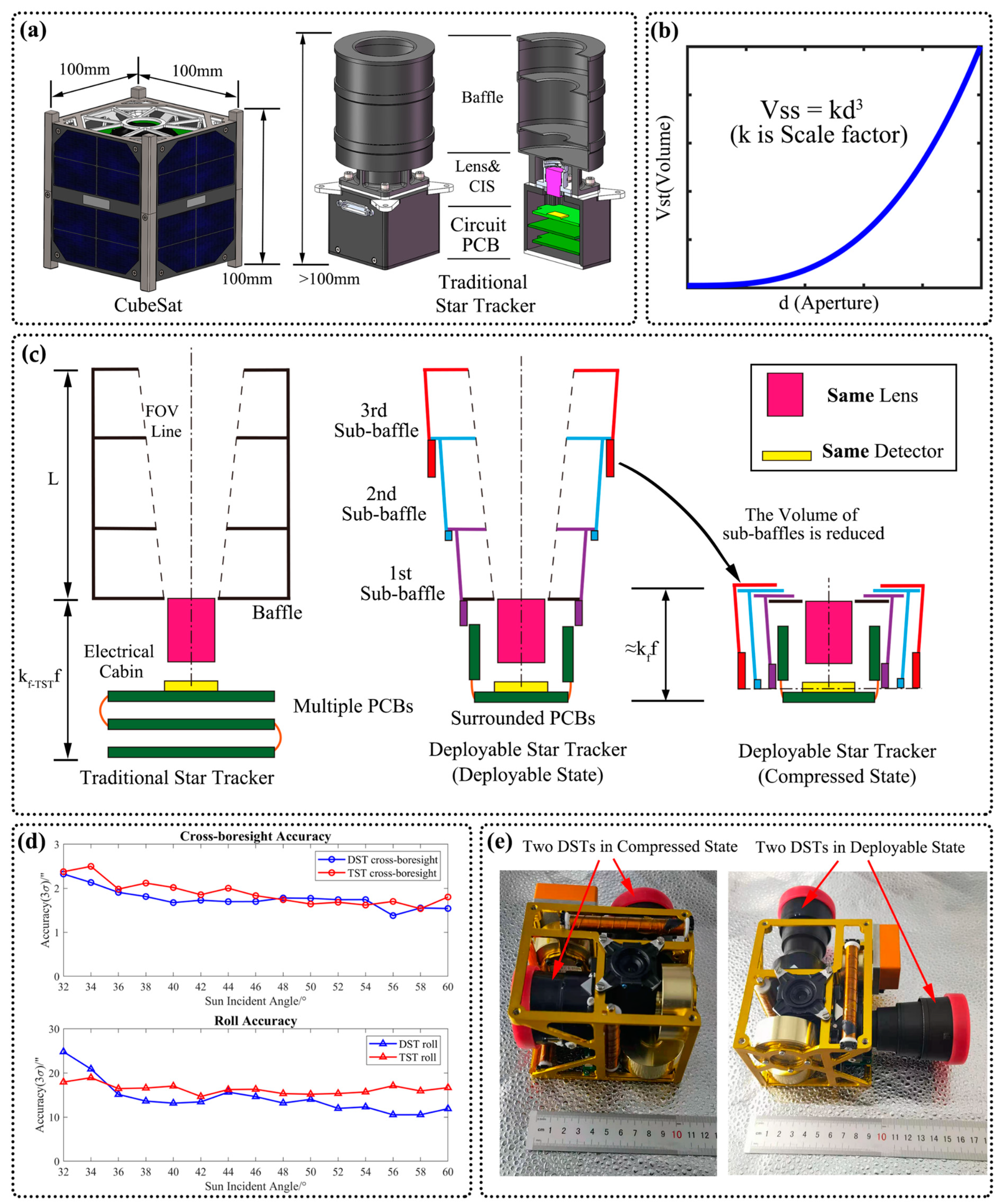
where $F_{lens}$ denotes the F-number of lens, $k_d$ denotes the ratio between the manufacturing diameter and the outer aperture diameter and $k_{f-TST}$ denotes the coefficient describing the relationship between the focal length and the length of the electronic cabin. It is obvious from the Equation (11) that the volume of traditional star tracker is cubic with the aperture of the lens.

To sum up, as is shown Figure 6, improving the pointing accuracy and dynamic performance of the star tracker will increase the aperture, which will further increase the length of the baffle and eventually increase the volume of the star tracker. If the volume of the baffle can be compressed by using an optimization model according to Equation (11), the length of the star tracker will be independent of the baffle no matter how the aperture is increased.

4. The Optimization Model and Analysis for the Deployable Star Tracker

4.1. Structure Design and Volume Analysis

The biggest difference between the DST and the TST is the deployable baffle structure. Given the aperture of lens and the half-FOV, the theoretical length of the baffle and the outer aperture can be calculated. The baffle of DST is divided into sub-baffles with different diameters by the vanes based on the geometrograph method [29]. Therefore, each sub-baffle can be nested with one another to achieve deployment and compression. The design method of deployable baffle is as follows.

In Figure 7, the positions of point A$\left(0,d/2\right)$, A’$\left(0,-d/2\right)$, B$\left(L,D/2\right)$ and B’$\left(L,-D/2\right)$ are known. Each theoretical sub-baffle’s diameter, $d_i^{\prime }\left(i=1,2,3\right),$ should be determined first. In order to reduce the diameter of DST in practical manufacturing, two vanes are employed in the proposed deployable baffle. The position point, $C\left(x_C,y_C\right)$, of first vane and the position point, $G\left(x_G,y_G\right)$, of the second vane can be determined by the geometrograph method. Point $H\left(x_H,y_H\right)$ is the intersection of line $A^{\prime }G$ and the outer aperture. Point $F\left(x_F,y_F\right)$ is the intersection of line $A^{\prime }C$ and line $B^{\prime }G$. The linear equations of line $AB$, line $B^{\prime }C$, line $A^{\prime }C$, line $B^{\prime }G$ and line $A^{\prime }G$ are as follows.

$$\{\begin{array}{l}{y}_{AB}=\frac{D-d}{2L}x+\frac{d}{2}\hfill \\ y_{B^{\prime }C}=-xtan\omega +Ltan\omega -\frac{D}{2}\hfill \\ y_{A^{\prime }C}=\frac{2y_c+d}{2x_c}x-\frac{d}{2}\hfill \\ y_{B^{\prime }G}=\frac{D+2y_F}{2\left(x_F-L\right)}x-\frac{2y_{F}L+D{x}_F}{2\left(x_F-L\right)}\hfill \\ y_{A^{\prime }G}=\frac{\left(2y_G+d\right)}{2x_G}x-\frac{d}{2}\hfill \end{array}$$

(12)

Point $H$ must satisfy Equation (13) to cancel the third vane.

$$y_H=\frac{L\left(2y_G+d\right)-d{x}_G}{2x_G}\le \frac{d_3^{\prime }}{2}$$

(13)

Each designed sub-baffle sidewall is different from the traditional baffle, which has a certain taper $\alpha$. The three important deployable baffle position parameters (point C, G and F) can be derived by Equation (12). Equation (14) represents the coordinates of point $C\left(x_C,y_C\right)$.

$$\{\begin{array}{l}{x}_c=\frac{2L^{2}tan\omega -L\left(D+d\right)}{D-d+2Ltan\omega }\hfill \\ y_c=\frac{\left(Dd-D^2+2DLtan\omega \right)}{2\left(D-d+2Ltan\omega \right)}\hfill \end{array}$$

(14)

Equation (15) represents the coordinates of point $G\left(x_G,y_G\right)$.

$$\{\begin{array}{l}{x}_G=\frac{L\left[L{d}_2^{\prime }+D{x}_F+d\left(x_F-L\right)\right]}{L\left(D+d_2^{\prime }\right)-\left(x_F-L\right)\left(D-d\right)}\hfill \\ y_G=\frac{D+d_2^{\prime }}{2\left(x_F-L\right)}{x}_G-\frac{L{d}_2^{\prime }+D{x}_F}{2\left(x_F-L\right)}\hfill \end{array}$$

(15)

Equation (16) represents the coordinates of point $F\left(x_F,y_F\right)$ in the following:

$$\{\begin{array}{l}{x}_F=\frac{d_2^{\prime }+d}{2y_c+d}{x}_c\hfill \\ y_F=\frac{d_2^{\prime }}{2}\hfill \end{array}$$

(16)

where $\omega$ denotes the sun aspect angle, $L$ denotes the theoretical length of the baffle and $D$ denotes the diameter of the outer aperture.

Any sub-baffle is independent with one another and driven by the springs. The springs are placed between the sub-baffles, as shown in Figure 8. The sub-baffles can be compressed by the external binding device and the springs are compressed between the sub-baffles. When the binding device is released, the sub-baffles will pop out and be deployed by the drive of the springs.

As shown in Figure 8a, each sub-baffle is divided into main body part $A_i$ and connection part $B_i$, $i=1,2,3$. $B_i$ is used to prevent the sub-baffle from being deployed excessively. As shown in Figure 8b, $B_i$ can make each sub-baffle coincide with the bottom to improve the stability after compression. The diameter and height of $A_i$ and $B_i$ must satisfy the constraint given by Equation (17) in the following:

$$tan\alpha =\frac{D_i-d_i}{2H_i}=\frac{D_{Bi}-d_{Bi}}{2p_i}$$

(17)

where α denotes the taper of the sub-baffle wall, $D_i$ denotes the inner diameter for the big end of $A_i$, $d_i$ denotes the inner diameter for the small end of $A_i$, $H_i$ denotes the distance between adjacent sub-baffle in the deployable state, $D_{Bi}=D_{i-1}$ denotes the inner diameter of the big end of $B_i$, $d_{Bi}$ denotes the inner diameter of the small end of $B_i$ and $p_i$ denotes the contact length between $B_i$ and $A_{i-1}$.

The most important parameters of the deployable baffle are the diameter and length of each sub-baffle. The structural parameters of $A_i$ satisfies the constraint as described in Equation (18):

$$U_{structure}=U_{theory}+\phi U_{baffle}$$

(18)

where $U_{structure}={\left[\begin{array}{cccccc}{d}_1& d_2& d_3& H_1& H_2& H_3\end{array}\right]}^T$ denotes the structure parameter of the deployable baffle, $U_{theory}={\left[\begin{array}{cccccc}{d}_1^{\prime }& d_2^{\prime }& d_3^{\prime }& 0& 0& 0\end{array}\right]}^T$ denotes the theoretical parameter of deployable baffle, $U_{baffle}={\left[\begin{array}{cccc}{x}_C& x_F& x_G& L\end{array}\right]}^T$ denotes design the parameter of deployable baffle and $\phi$ denotes the deign matrix of deployable baffle as is shown in Equation (19).

$$\phi =\left[\begin{array}{cccc}0& 0& 0& 0\\ -2tan\alpha & 2tan\alpha & 0& 0\\ 0& 0& 0& 0\\ 1& 0& 0& 0\\ -1& 0& 1& 0\\ 0& 0& -1& 1\end{array}\right]$$

(19)

To ensure that the $D_{Bi}$ of each sub-baffle can come into contact with the bottom surface due to the springs, each sub-baffle needs to satisfy the constraint as described in Equation (20) in the compressed state:

$$L_M+{\displaystyle \sum }_{k=1}^i{h}_k=H_i+l_i$$

(20)

where $L_M$ denotes the height of the lens mount, $h_i$ denotes the distance between adjacent sub-baffle in the suppression state, $l_i$ denotes the length of $B_i$, $l_i=l_{xi}+l_{yi}$, $l_{xi}$ denotes the length of $B_i$ with each sub-baffle and $l_{yi}$ is used to ensure that the bottom end of $B_i$ coincides with the bottom, respectively. In the actual mechanical design and processing, $h_i$ could be short by the design. When the signal processing circuit PCBs are complex, the PCBs are surrounded outside the lens to make full use of the space, as shown in Figure 8. Moreover, using SoC technology for signal processing can further reduce the number of circuit PCBs. Under the extreme and ideal conditions, the deployable length $L_d$ and compressed length $L_c$ of the deployable star tracker can be expressed as described in Equation (21):

$$\{\begin{array}{l}{L}_d=k_{f}f+L\hfill \\ L_c=k_{f}f\hfill \end{array}$$

(21)

where $k_f$ is similar to $k_{f-TST}$ in describing the DST. Combining with Equations (9) and (10), the volume of DST under deployable state and compressed state can be expressed as described in Equation (22).

$$\{\begin{array}{l}{V}_{DST-c}=\pi {\left(\frac{k_{d}D}{2}\right)}^{2}L=\frac{\pi k_d^2{k}_2^2{k}_f{F}_{lens}}{4}{d}^3\hfill \\ V_{DST-d}=\pi {\left(\frac{k_{d}D}{2}\right)}^2\left(L+k_{f}f\right)=\frac{\pi k_d^2{k}_2^2\left(1+k_1{k}_f{F}_{lens}\right)}{4k_1}{d}^3\hfill \end{array}$$

(22)

The volume ratio $\kappa$ of compression to deployment is as described in Equation (23).

$$\kappa =\frac{V_{DST-c}}{V_{DST-d}}=\frac{k_1{k}_f{F}_{lens}}{1+k_1{k}_f{F}_{lens}}$$

(23)

Therefore, compared with the TST, the DST can effectively reduce its volume in a special manner.

4.2. Analysis of Reliability

When the baffle is being deployed, the deploying time of the same sub-baffle with different edges may be different. The springs will be deformed so that the driving force is not along the optical axis. No matter how much driving force the springs produce, the sub-baffles cannot continue in its deployment, which is named as the baffle self-lock phenomenon. In order to solve the self-lock problem, it is assumed that the sub-baffle $i$ inclines for some reason during the deployment with $\beta$ angle relative to the sub-baffle $i-1$. Additionally, it is assumed that the spring driving force $T$ is along the optical axis of the sub-baffle $i$ and the stress model of the sub-baffle is shown in Figure 9.

When the sub-baffle $i$ is stationary, the stress relationship is as described in Equation (24):

$$\{\begin{array}{c}{f}_{2}cos\left(\alpha +\beta \right)+f_{1}cos\left(\beta -\alpha \right)=Tcos\beta \\ f_{2}sin\left(\alpha +\beta \right)+f_{1}sin\left(\beta -\alpha \right)=Tsin\beta \end{array}$$

(24)

where $f_1$ and $f_2$ denote the friction force on the upper and lower edge of the sub-baffle $i$ as Figure 9. The definition of friction is given by $f_1=\mu N_1$ and $f_2=\mu N_2$ (μ is the friction coefficient between the sub-baffle). $N_1$ and $N_2$ are the positive pressures of the sub-baffle $i$ on the upper and lower edge of the sub-baffle $i-1$, respectively. $F_1$ and $F_2$ are the positive pressures of the sub-baffle $i-1$ on the upper and lower edge of the sub-baffle $i$, respectively. According to the geometric relationship of the force, Equation (25) can be derived.

$$F_1=F_2=F=\frac{T}{2sin\alpha }$$

(25)

Combined with Equations (24) and (25), the critical condition of self-lock can be derived as Equation (26).

$$tan\alpha =\mu$$

(26)

Therefore, in order to prevent the self-lock during deployment, the taper and friction coefficient of the sub-baffle must satisfy $tan\alpha >\mu$, which can be considered to possess high reliability.

4.3. Analysis of Deployment Accuracy

The inclination between sub-baffles may occur after deployment because the spring force is not completely along the optical axis. If the adjacent sub-baffle inclines after full deployment, the imaging and stray light suppression ability for the star tracker will be affected due to the incorrect position of the sub-baffles.

In the worst case, with a force perpendicular to the sidewall in the deployable state, the fit clearance error in the manufacturing process will cause the relative inclination of adjacent sub-baffle. The material of the baffle will deform to cause further inclination. It is assumed that the fit clearance between adjacent sub-baffle is $\Delta m\ge 0$ and the adjacent sub-baffles are inclined relatively under the action of external forces as shown in Figure 10.

If the fit clearance satisfies $\Delta m=0$, it must be considered that the angle between the sub-baffle and the radius of the rotating circle is greater than ${90}^{°}$. Otherwise, the sub-baffles would also be inclined under $\Delta m=0$. Therefore, the contact length $p_i$ must satisfy Equation (27).

$$p_i>D_{i}sin\alpha$$

(27)

If Equation (27) is satisfied, it can ensure zero inclination when achieving full deployment without applying force. Only when this condition is satisfied will the influence of the fit clearance $\Delta m$ on the inclination be considered.

When the fit clearance satisfies $\Delta m>0$ and Equation (27), respectively, the sub-baffle $i$ inclines relative to the sub-baffle $i-1$ under the action of external force as shown in Figure 10b. In triangle ACG, Equation (28) can be derived by the cosine theorem described as follows:

$$S^2+{\left(R-\Delta \right)}^2-2S\left(R-\Delta \right)cos\left(90+\beta -\alpha \right)=R^2$$

(28)

where $S$ denotes the length of line CG, $R$ denotes the length of line AG and AC, $\Delta =\frac{R}{\left(D+\Delta m\right)}\Delta m$ denotes the length of line BC and $\beta$ is angle of $\mathrm{CAF}$. Therefore, the S is derived as described in Equation (29).

$$S=\left(R-\Delta \right)sin\left(\alpha -\beta \right)+\sqrt{{\left(R-\Delta \right)}^{2}si{n}^2\left(\alpha -\beta \right)+\Delta \left(2R-\Delta \right)}$$

(29)

The maximum inclination angle ${\gamma }_i$ can be derived as described in Equation (30).

$$sin{\gamma }_i=\frac{S}{R}cos\left(\beta -\alpha \right)$$

(30)

To simplify the expression of ${\gamma }_i$, the $R$ and $\beta$ must be reduced. In triangle ACF, the Equation (31) can be derived by the sine theorem.

$$\frac{p_i}{sin\beta }=\frac{R}{sin\left(90-\alpha \right)}=\frac{D_i+\Delta m}{sin\left(90+\alpha -\beta \right)}$$

(31)

Therefore, $sin\beta$ and $cos\beta$ can be derived as described by Equation (32).

$$\{\begin{array}{l}sin\beta =\frac{p_{i}cos\alpha }{R}\hfill \\ cos\beta =\frac{D_i+\Delta m-psin\alpha }{R}\hfill \end{array}$$

(32)

In triangle ACF, the Equation (33) can be derived by the cosine theorem.

$$R^2=p^2+{\left(D+\Delta m\right)}^2-2p\left(D+\Delta m\right)sin\alpha$$

(33)

Combining Equations (29), (30), (32) and (33), the maximum inclination angle ${\gamma }_i$ between adjacent sub-baffles can be derived as described in Equation (34):

$${\gamma }_i=arcsin\left({\delta }_i{\lambda }_i{\xi }_i+{\xi }_i\sqrt{{\delta }_i{\lambda }_i^2+\left(1-{\delta }_i^2\right)}\right)$$

(34)

where the following equations apply as described.

$${\delta }_i=\frac{D_i}{D_i+\Delta m}$$

(35)

$${\lambda }_i=\frac{\left(D_i+\Delta m\right)sin\alpha -p_i}{\sqrt{p_i^2+{\left(D_i+\Delta m\right)}^2-2p_i\left(D_i+\Delta m\right)sin\alpha }}$$

(36)

$${\xi }_i=\frac{\left(D_i+\Delta m\right)cos\alpha }{\sqrt{p_i^2+{\left(D_i+\Delta m\right)}^2-2p_i\left(D_i+\Delta m\right)sin\alpha }}$$

(37)

The total maximum inclination angle $\gamma$ of the three-stage sub-baffle relative to the lens center is described in Equation (38).

$$\gamma ={\displaystyle \sum }_{i=1}^3{\gamma }_i$$

(38)

With the external force, the three sub-baffles can be regarded as interference joints when the fit clearance satisfies $\Delta m=0$. The whole deployable baffle can be regarded as a rigid body and cantilever structure. When the fit clearance satisfies $\Delta m>0$, the three sub-baffles will incline first. Then the material deformation occurs and each sub-baffle can be regarded as a cantilever structure separately. Due to the irregular shape of the sub-baffles, the finite element method (FEM) software will be used to analyze the material deformation of the deployable baffle under the two fit conditions.

5. Results

5.1. Volume Ratio

Table 1. The key values of the DST and the ideal ratios value for volume.

Index	Value
$F_{lens}$	1.7453
$k_1$	0.187643
$k_f$	2.00
${\kappa }_{ideal}$	0.40
${\kappa }_{real}$	0.44

lists the key values related to the volume ratio and the calculated ratio values according to the Equation (22). Due to the requirements of manufacturing technology and space radiation protection, the length of the deployable baffle with a small focal length after compression cannot be completely ignored. Therefore, the real volume ratio ${\kappa }_{real}$ is slightly larger than the ${\kappa }_{ideal}$.

If the focal length is larger, then the two values of volume ratio will be closer. The DST can be smaller and closer to the volume limitation by optimizing the structure in the future.

5.2. Deployment Accuracy and Reliability

The deployment accuracy of the DST is mainly affected by the inclination and material deformation of the sub-baffles. The relevant design parameters of the practical DST are shown in

Table 2. The relevant design parameters of sub-baffles.

Index	${\mathit{p}}_{\mathit{i}}/\mathbf{mm}$	${\mathit{D}}_{\mathit{i}}/\mathbf{mm}$
The 1st sub-baffle	3.007	31.11
The 2nd sub-baffle	3.649	37.41
The 3rd sub-baffle	3.007	44.37

. It is explained that the simulations are based on the parameters of practical DST.

The relationship between the relative maximum inclination angle and the clearance for each sub-baffle of the proposed DST is calculated by Equation (34), as shown in Figure 11. The simulation results show that the relative maximum inclination angle between the sub-baffles can be greatly reduced with the smaller clearance value.

As shown in Figure 12, the material deformation analysis with $\Delta m=0$ and $\Delta m=0.1 \mathrm{mm}$ after deployment of the practical DST is realized by the FEM software, ANSYS. A vertical force of 100 Mpa is applied to the edge of the third sub-baffle. The relevant simulation parameters and results are shown in

Table 3. The relevant simulation parameters and results for deployable baffle with $\Delta m=0$ and $\Delta m=0.1\mathrm{mm}$.

Index	$\mathbf{\Delta }\mathit{m}=0$	$\mathbf{\Delta }\mathit{m}=0.1\mathbf{mm}$
Material	AL 2024-T4	AL 2024-T4
Young’s modulus	73,000 Mpa	73,000 Mpa
Poisson’s ratio	0.33	0.33
Max deformation	$6.98\times {10}^{-4}$	$4.11\times {10}^{-4}$ m

. The simulation results show that the material deformation can be ignored because the values of two $\Delta m$ are both less than 1 mm. Therefore, for the sake of deployment accuracy, only the influence of inclination for sub-baffles needs to be considered.

In order to avoid self-lock, the taper of the designed sub-baffles must satisfy $\mathsf{\alpha }>{2.86}^{°}$ as described in Equation (26) by polytetrafluoroethylene (PTFE) with $\mu =0.05$. The practical design of the sub-baffles has a taper of $4^{°}$. However, by conducting deployment experiments 50 times for the practical DST without PTFE as shown in Figure 13, the experimental results show that each sub-baffle can be deployed to the appropriate position without self-lock and the average height error of the DST is 0.0284 mm within the allowable error range. Therefore, the inclination between adjacent sub-baffles can be approximately ignored.

5.3. Environmental Adaptability

The space temperature will be extreme when the DST is deploying. The deploying device system requires heat to release the sub-baffles. It is necessary to consider whether the DST can be deployed at extremely low temperatures. Thus, ten experiments were carried out at extremely low temperatures ($-40$ °C) and room temperature ($25$ °C), respectively. The experiment results show that the DST can be deployed at extremely low temperature, which takes ${\overline{t}}_{-40{ }^{°}\mathrm{C}}=243.6 \mathrm{s}$ from the moment of sending the deployment command to full deployment. However, it only takes ${\overline{t}}_{25{ }^{°}\mathrm{C}}=32.3 \mathrm{s}$ at room temperature. Although the deployment time of the DST at extremely low temperatures is much longer than that at room temperature, it proves that the deployable baffle can finally be deployed in space environment.

Due to the satellite attitude, the top and circumferential direction of the star tracker will be directly illuminated by the sun during a certain period of time after the satellite enters the sunlight area. If the black anodizing process is adopted, the sun absorption rate of the baffle is high and the temperature will rise rapidly. After entering the shadow area, the temperature will decrease rapidly, resulting in a great temperature fluctuation. In practical satellite applications, as shown in Figure 14, silvered fluorinated ethylene propylene film (also known as F46/Ag film) is pasted on the surface of the deployable baffle because it has much lower sun absorptance.

According to the mass and heat capacity of the satellite as shown in Figure 14,

Table 4. The temperature changes of black anodizing process and F46/Ag film in an orbital cycle.

Index	Black Anodizing	F46/Ag Film
DST-1	$-2~48$(°C)	$-4~24$(°C)
DST-2	$-1~49$(°C)	$-2~29$(°C)

shows the results of temperature changes relative to whether or not the DST has F46/Ag film pasted in an orbital cycle. The F46/Ag film can greatly reduce the influence of the sun on DSTs, rendering the DSTs with better environmental adaptability.

5.4. Stray Light Suppression Ability

For the DST, the deployable structure does not affect its optical performance. The point light transmittance (PST) is usually used to measure the ability of the baffle to suppress stray light. The PST is defined as the ratio of the illuminance $E_o\left(\theta \right)$ generated on the imaging surface of the optical detector and the illuminance $E_i\left(\theta \right)$ on the input aperture perpendicular to the point source as described in Equation (31), when a light source with an off-axis angle of $\theta$ passes through the optical system.

$$PS{T}_{\theta }=\frac{E_o\left(\theta \right)}{E_i\left(\theta \right)}$$

(39)

For the star tracker, the illuminance of the sunlight at the entrance of the baffle is constant except in the shadow areas of Earth. The simulation results of the deployable baffle and the traditional baffle with the same optical parameters are shown in Figure 15. The optical absorbance of the coating material on the inner surface is set to 95%. The design sunlight suppression angle is ${28}^{°}$.

The simulation results show that the stray light suppression ability of the deployable baffle is as good as a traditional baffle. In order to achieve the practical PST performance of the baffle, an experiment was carried out, as shown in the Figure 16a. The ultrablack film with absorbance up to $95\%$ is coated on the inner surface of sub-baffles. The practical DST was rotated to create a certain angle with the fixed sun simulator to simulate the stray light incident angle. The stray light incident angle is set to 28° to 60° (interval of 2°). At different stray light incident angles, the average background gray values of the 1000 images are recorded, respectively.

According to the average gray values of the images under different sun incident angles, the normalized test result of PST was achieved and the simulation result was also normalized as Figure 16b. The experiment results possess a similar curve as the simulations, which means the deployable baffle has good stray light suppression ability.

5.5. Accuracy and Dynamic Performance

As shown in Figure 16a, in order to acquire the accuracy of star trackers at different sun incident angles, the 1000 quaternion data are calculated by the star tracker in real time at each sun incident angle. Due to the weather, only 32° to 60° experimental data are adopted. According to the quaternion differential equation as described in Equation (40), the three-axis angular velocity of star tracker can be calculated as follows:

$$\frac{dQ}{dt}=\frac{1}{2}Q\otimes {\omega }_{Rb}^b$$

(40)

where $Q={\left[\begin{array}{cccc}{q}_0& q_1& q_2& q_3\end{array}\right]}^T$ denotes the attitude quaternion and ${\omega }_{Rb}^b$ denotes the rotational angular velocity of the star tracker, respectively. Due to the short sampling time for calculations, the three-axis rotation angle of the star tracker can be calculated by using Equation (41):

$${\theta }^{\left(k\right)}\approx \frac{1}{2}{Q}^{\left(k\right)}\otimes \left(Q^{\left(k+1\right)}-Q^{\left(k\right)}\right)$$

(41)

where $Q^{\left(k\right)}$ denotes the quaternion at time k and ${\theta }^{\left(k\right)}$ denotes the three-axis rotation angle of the star tracker between time k and time k − 1. Since the star tracker does not rotate on the tripod, the three-axis rotation angle should be zero, theoretically. However, the measured three-axis rotation angle is not zero. The triple standard deviation ($3\sigma$) method is adopted to evaluate the accuracy of the star tracker. It should be explained that because the calculated rotation angle is positive, its probability density function is different from that of Gaussian distribution [30]. The result must be divided by the $\sqrt{2}$.

The predicted accuracy ($3\sigma$) of star trackers can be expressed by the noise equivalent angle (NEA). The calculation equations of NEA are described as Equation (42) [31]. The roll axis error angle of the star tracker will be affected by the focal length. Therefore, the NEA of roll axis will be worse than that of cross-boresight. The equation is described as follows:

$$\{\begin{array}{l}{E}_{cross-boresight}=\frac{{\theta }_{FOV}·E_{centroid}}{N_{e\_pixel}·\sqrt{N_{star}}}\hfill \\ E_{roll}=atan\left(\frac{E_{centroid}}{0.3825·N_{e\_pixel}}\right)·\frac{1}{\sqrt{N_{star}}}\hfill \end{array}$$

(42)

where $N_{e\_pixel}$ denotes the number of effective pixels, $E_{centroid}$ denotes the average centering accuracy and $N_{star}$ denotes the average number of recognized stars. The design parameters and predicted accuracy of the DST are shown in

Table 5. The design parameters and predicted accuracy of the DST.

Index	Value
${\theta }_{FOV}$	${20}^{°}$
$E_{centroid}$	$0.1 pixel$
$N_{e\_pixel}$	$1292 pixel$
$N_{star}$	$12$
$E_{cross-brosight}$	${1.61}^{″} \left(3\sigma \right)$
$E_{roll}$	${12.05}^{″}\left(3\sigma \right)$

.

The practical accuracy ($3\sigma$) variation between the proposed DST and TST with the same lens and detector under different sun incident angles is shown in Figure 17. The three-axis average accuracy ($3\sigma$) is shown in

Table 6. The cross-boresight and roll axis average accuracy ($3\sigma$) for two star trackers.

Index	Cross-Boresight $\left(3\mathit{\sigma }\right)$	Roll $\left(3\mathit{\sigma }\right)$
DST average	${1.76}^{″}$	${14.38}^{″}$
TST average	${1.89}^{″}$	${16.36}^{″}$

.

The average accuracy of the DST is better than 2″ $\left(3\sigma \right)$. However, in the whole experiment, the accuracy of the DST is better than 3″ $\left(3\sigma \right)$. Due to the influence of weather and the installation in the experiment, the accuracy of the two star trackers is somewhat different. However, it is within the allowable error range. When the sun incident angle is close to the designed sunlight suppression angle, the accuracy of DST and TST becomes simultaneously worse. Although the energy of the stars is greater than the stray light, the gray values of the stars becomes higher. The centroid method for extracting the stars would result in the offset of the star coordinates. This problem can be solved if a more advanced star extraction algorithm is adopted.

It should be explained that the accuracy of the DST is the measurement accuracy of the instrument at that time and environment. If the absolute attitude data of the star tracker needs to be obtained, some important factors such as chromatic aberration, temperature, stellar aberrations and proper motion should be further considered [32]. The lens of the DST has completed the correction of distortion and chromatic aberration. Bulk thermal changes can be corrected by on-orbit recalibration. Stellar aberrations and proper motion can be corrected by an accurate real-time clock and orbital ephemeris.

The remote sensing CubeSats usually do not regard the dynamic performance as important and so the designed parameters about the lens and detector are mainly focused on accuracy. The DST and TST are fixed on a uniaxial turntable without stray light and the turntable rotates at a constant slew rate within $\pm {10}^{°}$, as shown Figure 18. The rotation angular velocity of the star tracker can be calculated by Equation (40). The slew rate is constant and so the angular calculated by Equation (41) increased and decreased uniformly. The triple standard deviation ($3\sigma$) of the angular is adopted to evaluate the accuracy.

The uniaxial turntable is rotated at 0.5, 1.0, 1.5, 2.0, 2.5 and 3.0°/s in dynamic performance experiments. The calculated slew rate by two star trackers is shown in Figure 19. The average accuracy ($3\sigma$) under different slew rates is shown in

Table 7. The average accuracy ($3\sigma$) for DST and TST under slew rate of 0.5, 1.0, 1.5, 2.0, 2.5 and 3.0°/s.

Slew Rate (°/s)	DST Average Accuracy $\left(3\mathit{\sigma }\right)$	TST Average Accuracy $\left(3\mathit{\sigma }\right)$
0.5	3.38″	3.84″
1.0	6.08″	6.07″
1.5	9.87″	9.06″
2.0	11.43″	11.66″
2.5	16.88″	17.50″
3.0	27.16″	27.34″

.

The dynamic performance experiments show that the DST and the TST with same lens and detector are similar. The DST and the TST can both identify the stars under the maximum slew rate of 3°/s. The reason why the accuracy of the star trackers decreases with the increase in slew rate is that the star spots are trailing as shown in Figure 3, which results in the offset of star spots centroid.

6. Discussion

In this paper, an on-orbit DST is proposed. The DST with high accuracy and small volume is realized by the deployable baffle and surrounding circuit structure. On the one hand, any large and high-accuracy star tracker such as ASTRO-15 can use the proposed model to reduce its volume. On the other hand, the designers can only focus on the volume of the lens and detector to make star trackers smaller and more accurate.

If there is difficulty in deploying the DST due to extreme space temperature, the satellite could send the deployment command for a longer period of time to allow the heating resistors to fuse the nylon wire. The satellite could also rely on other attitude sensors, such as sun sensors, when the DST could not be deployed. If the space temperature is appropriate, the satellite could send deployment commands. Actually, a satellite is usually equipped with more than two star trackers. If one of them could not be deployed, the others could be deployed successfully. If all the DSTs are not deployed for some reason, it does not mean that the DSTs cannot work. The result of this impact is that the ability of the baffle to suppress stray light will be weakened. The satellite requires readjustment to their attitude to ensure that stray light does not enter the FOV of the DST.

The DST can be used in IADCS designed for CubeSats. Compared with the IADCS400 [33] designed by Hyperion Technologies, the example IADCS can equip two DSTs as shown in Figure 20 such that the occupation of TST is greatly reduced. Moreover, the attitude determination accuracy with 3″ (3σ) of the example IADCS is much higher than IADCS400 with 30″ (3σ). Additionally, the DST can further reduce the rocket launch volume occupied by the star tracker. After the CubeSat enters the orbit, it can be deployed to release the space. The CubeSat would be subjected to certain spring forces during deployment, which can cause the satellite to rotate or deviate from its orbit. However, the IADCS can drive the reaction wheels or the propellers to solve that problem at this moment.

With future optimizations, the volume of DST can be further reduced to the volume limit. Thus, the high-accuracy satellite could be much smaller to reduce the launch volume and cost significantly. More and more organizations and companies would launch CubeSats to build their own constellation for scientific research or commercial viability.

7. Conclusions

By analyzing the relationship between volume and accuracy or dynamic performance, this paper proposed an on-orbit DST. The deployable baffles with a scientifically analyzed and verified taper and surrounding circuit structure are designed to minimize the volume of the star tracker. The experiment results show that the practical DST has a volume ratio close to the theoretical value. The simulations and experiments show that it can be deployed with an error close to zero and without self-locking risk due to the taper and a series of strategies. Furthermore, the DST can even be deployed in extreme temperatures so that the DST would not be affected by the temperatures common to space environments. Compared to the TST with same lens and detector, the stray light suppression ability, accuracy (better than 3″ $\left(3\sigma \right)$) and dynamic performance (up to 3°/s) are nearly equal. More than one DST can easily be integrated in IADCS for CubeSats to provide high-accuracy attitude data for remote sensing applications.

References

1. Van der Meer, F.D.; Van der Werff, H.M.; Van Ruitenbeek, F.J.; Hecker, C.A.; Bakker, W.H.; Noomen, M.F.; Van Der Meijde, M.; Carranza, E.J.M.; De Smeth, J.B.; Woldai, T. Multi-and hyperspectral geologic remote sensing: A review. Int. J. Appl. Earth Obs. Geoinf. 2012, 14, 112–128. [Google Scholar] [CrossRef]
2. Ma, Y.; Xu, R. Remote sensing monitoring and driving force analysis of urban expansion in Guangzhou City, China. Habitat Int. 2010, 34, 228–235. [Google Scholar] [CrossRef]
3. Sei-Ichi, S.; Robinson, M.; Nyoman, R.I.; Shinsuke, A.; Fumihiro, T.; Toru, H.; Yoichi, I.; Toshiyuki, A.; Teiji, I.; Shigeki, S. Some operational uses of satellite remote sensing and marine GIS for sustainable fisheries and aquaculture. ICES J. Mar. Sci. 2011, 68, 687–695. [Google Scholar]
4. Ayad, Y.M. Remote sensing and GIS in modeling visual landscape change: A case study of the northwestern arid coast of Egypt. Landsc. Urban Plan. 2005, 73, 307–325. [Google Scholar] [CrossRef]
5. Atzberger, C. Advances in remote sensing of agriculture: Context description, existing operational monitoring systems and major information needs. Remote Sens. 2013, 5, 949–981. [Google Scholar] [CrossRef] [Green Version]
6. Weng, Q. Thermal infrared remote sensing for urban climate and environmental studies: Methods, applications, and trends. ISPRS J. Photogramm. Remote Sens. 2009, 64, 335–344. [Google Scholar] [CrossRef]
7. Mahmoud, A.A.; Elazhary, T.T.; Zaki, A. Remote sensing cubesat. In Sensors, Systems, and Next-Generation Satellites XIV, Proceedings of the Spie Remote Sensing, Toulouse, France, 20–23 September 2010; SPIE: Bellingham, WA, USA, 2010; p. 78262. [Google Scholar]
8. Puig-Suari, J.; Turner, C.; Ahlgren, W. Development of the standard CubeSat deployer and a CubeSat class PicoSatellite. In Proceedings of the 2001 IEEE Aerospace Conference Proceedings (cat. No. 01TH8542), Big Sky, MT, USA, 10–17 March 2001; Volume 1, pp. 1/347–1/353. [Google Scholar]
9. Villela, T.; Costa, C.A.; Brandão, A.M.; Bueno, F.T.; Leonardi, R. Towards the thousandth Cubesat: A statistical overview. Int. J. Aerosp. Eng. 2019, 2019, 1–13. [Google Scholar] [CrossRef]
10. Foster, C.; Hallam, H.; Mason, J. Orbit determination and differential-drag control of planet LABS Cubesat constellations. In Astrodynamics 2015; Majji, M., Turner, J.D., Wawrzyniak, G.G., Cerven, W.T., Eds.; Univelt: Escondido, CA, USA, 2016; Volume 156, pp. 645–657. [Google Scholar]
11. Nagel, G.W.; Novo, E.M.L.d.M.; Kampel, M. Nanosatellites applied to optical earth observation: A review. Rev. Ambient. Água 2020, 15, 2513. [Google Scholar] [CrossRef]
12. Wang, H.; Zhou, W.; Cheng, X.; Lin, H. Image smearing modeling and verification for strapdown star sensor. Chin. J. Aeronaut. 2012, 25, 115–123. [Google Scholar] [CrossRef] [Green Version]
13. Eisenman, A.R.; Liebe, C.C.; Joergensen, J.L. New generation of autonomous star trackers. Proc. SPIE Int. Soc. Opt. Eng. 1997, 3221, 524–535. [Google Scholar] [CrossRef]
14. Mortari, D.; Romoli, A.; Ieee, I. StarNav III: A three fields of view star tracker. In Proceedings of the 2002 IEEE Aerospace Conference Proceedings, Big Sky, MT, USA, 9–16 March 2002; Volumes 1–7, pp. 47–57. [Google Scholar]
15. Schmidt, U. Autonomous star tracker based on active pixel sensors (APS). In Proceedings of the 5th International Conference on Space Optics, Toulouse, France, 30 March–2 April 2004; Warmbein, B., Ed.; European Space Agency: Pairs, France, 2004; Volume 554, pp. 355–358. [Google Scholar]
16. Dzamba, T.; Enright, J.; Sinclair, D.; Amankwah, K.; Votel, R.; Jovanovic, I.; Mcvittie, G. Success by 1000 improvements: Flight qualification of the ST-16 star tracker. In Proceedings of the 28th AIAA/USU Conference on Small Satellites, Logan, UT, USA, 2–7 August 2014. [Google Scholar]
17. Sarda, K.; Grant, C.C.; Zee, R.E. Three stellar years (and counting) of precision photometry by the BRITE astronomy constellation. In Proceedings of the 30th AIAA/USU Conference on Small Satellites, Logan, UT, USA, 8–11 August 2016. [Google Scholar]
18. Kawano, H.; Shimoji, H.; Yoshikawa, S.; Miyatake, K.; Hama, K.; Nakamura, S. Optical testing of star sensor (I): Defocus spot measuring technique for ground-based test. Opt. Rev. 2008, 15, 110–117. [Google Scholar] [CrossRef]
19. Kawano, H.; Shimoji, H.; Yoshikawa, S.; Miyatake, K.; Hama, K.; Nakamura, S. Optical testing of star sensor (II): Alignment of star sensor from off-line pictures taken in orbital test. Opt. Rev. 2008, 15, 118–124. [Google Scholar] [CrossRef]
20. Wang, G.; Xing, F.; Wei, M.; You, Z. Rapid optimization method of the strong stray light elimination for extremely weak light signal detection. Opt. Express 2017, 25, 26175–26185. [Google Scholar] [CrossRef] [PubMed]
21. Cassidy, L.W. Miniature star tracker. In Proceedings of the Space Guidance, Control, and Tracking, Orlando, FL, USA, 12–14 April 1993. [Google Scholar]
22. Van Breukelen, E. Facet nano, a modular star tracker concept for highly miniaturized spacecraft. In Proceedings of the 60th International Astronautical Congress, Daejeon, Korea, 12–16 October 2009; pp. 12–16. [Google Scholar]
23. Pain, B.; Cunningham, T.; Nikzad, S.; Hoenk, M.; Jones, T.; Wrigley, C.; Hancock, B. A back-illuminated megapixel CMOS image sensor. In Proceedings of the IEEE Workshop on Charge-Coupled Devices and Advanced Image Sensors Karuizawa, Nagano, Japan, 9–11 June 2005. [Google Scholar]
24. Kumagai, O.; Niwa, A.; Hanzawa, K.; Kato, H.; Futami, S.; Ohyama, T.; Imoto, T.; Nakamizo, M.; Murakami, H.; Nishino, T. A 1/4-inch 3.9 Mpixel low-power event-driven back-illuminated stacked CMOS image sensor. In Proceedings of the 2018 IEEE International Solid-State Circuits Conference-(ISSCC), San Francisco, CA, USA, 11–15 February 2018; pp. 86–88. [Google Scholar]
25. Sukegawa, S.; Umebayashi, T.; Nakajima, T.; Kawanobe, H.; Koseki, K.; Hirota, I.; Haruta, T.; Kasai, M.; Fukumoto, K.; Wakano, T. A 1/4-inch 8Mpixel back-illuminated stacked CMOS image sensor. In Proceedings of the 2013 IEEE International Solid-State Circuits Conference Digest of Technical Papers, San Francisco, CA, USA, 17–21 February 2013; pp. 484–485. [Google Scholar]
26. Ju, G. Autonomous star sensing, pattern identification and attitude determination for spacecraft: An analytical and experimental study. Diss. Abstr. Int. 2001, 62–64, 1948. [Google Scholar]
27. Wahba, G. A least squares estimate of satellite attitude. SIAM Rev. 1965, 7, 409. [Google Scholar] [CrossRef]
28. Alexander, B.F.; Ng, K.C. Elimination of systematic-error in subpixel accuracy centroid estimation. Opt. Eng. 1991, 30, 1320–1331. [Google Scholar] [CrossRef]
29. Arnoux, J.J. Star sensor baffle optimization: Some helpful practical design rules. Proc. SPIE Int. Soc. Opt. Eng. 1996, 2864, 333–338. [Google Scholar] [CrossRef]
30. Jiao, Y.-Y.; Zhou, H.-Y.; Li, X.-N.; Wang, J.-Q.; Pan, X.-G. Cone measurement error model of star-sensor’s optic axis and its application. J. Astronaut. 2010, 31, 2138–2144. [Google Scholar]
31. Liebe, C.C. Accuracy performance of star trackers—A tutorial. IEEE Trans. Aerosp. Electron. Syst. 2002, 38, 587–599. [Google Scholar] [CrossRef]
32. Enright, J.; Sinclair, D.; Dzamba, T. The things you can’t ignore: Evolving a sub-arcsecond star tracker. In Proceedings of the 26th AIAA/USU Conference on Small Satellites, Logan, UT, USA, 13–16 August 2012. [Google Scholar]
33. The Descriptions and Specifications of IADCS400 Designed by Hyperion Technologies. Available online: https://hyperiontechnologies.nl/wp-content/uploads/2015/07/HT_iADCS400_v2.1-flyer.pdf (accessed on 15 December 2020).
Figure 1. (a) The comparison between the CubeSat(1U) with TST and the structure of TST. (b) The relationship between the volume and the aperture of the star tracker. (c) The proposed DST with deployable state and compressed state. (d) The accuracy between DST and TST under different sun incident angles. (e) The practical product of IADCS for CubeSats and DST in compressed state and deployable state, respectively.
Remotesensing 13 02503 g001
Figure 2. (a) v i in the celestial coordinate system. (b) Principle of the star tracker and w i in the star tracker coordinate system. (c) Pointing accuracy model of the star tracker.
Remotesensing 13 02503 g002
Figure 3. (a) Star coordinates extraction under strong stray light. (b) Star spot imaging with satellite rotating.
Remotesensing 13 02503 g003
Figure 4. Basic baffle design for length and outer aperture diameter.
Remotesensing 13 02503 g004
Figure 5. Baffle length with different half-FOV and the earth aspect angle.
Remotesensing 13 02503 g005
Figure 6. The volume relationship between pointing accuracy and dynamic performance.
Remotesensing 13 02503 g006
Figure 7. The deployable baffle design under the geometrograph method.
Remotesensing 13 02503 g007
Figure 8. (a) Deployed state of deployable star tracker. (b) Suppression state of deployable star tracker. (c) Detail view for the contact part.
Remotesensing 13 02503 g008
Figure 9. The stress model of the sub baffles and force analysis for deployable baffle.
Remotesensing 13 02503 g009
Figure 10. (a) The adjacent sub-baffles are deployed without external force. (b) The relative inclination model between sub-baffles for deployable baffle.
Remotesensing 13 02503 g010
Figure 11. Each sub-baffle inclination with different clearance values.
Remotesensing 13 02503 g011
Figure 12. (a) The material analysis at Δ m = 0.1   mm . (b) The material analysis at Δ m = 0 .
Remotesensing 13 02503 g012
Figure 13. The practical deployment height of the deployable baffle at 50 times experiment.
Remotesensing 13 02503 g013
Figure 14. Two deployable star trackers with slivered fluorinated ethylene propylene F46/Ag film on a Satellite (DST-1 is in the deployable state and DST-2 is in the compressed state).
Remotesensing 13 02503 g014
Figure 15. PST comparison between two type baffles with 28~90° sun angle (interval of 2°).
Remotesensing 13 02503 g015
Figure 16. (a) Practical stray light experiment for DST with sun simulator. (b) Normalized PST comparison between simulation and practical experiment (The normalized PST value is relative to the value of the sun angle of 28°).
Remotesensing 13 02503 g016
Figure 17. The variation of three-axis accuracy for two star trackers.
Remotesensing 13 02503 g017
Figure 18. The dynamic performance experiment. (a) The turntable is at + 10 ° . (b) The turntable is at 10 ° .
Remotesensing 13 02503 g018
Figure 19. (a) Measured angular velocity of the DST. (b) Measured angular velocity of the TST.
Remotesensing 13 02503 g019
Figure 20. An example IADCS with two DSTs. The IADCS also includes a sun sensor, a gyroscope, three reaction wheels and three magnetorquers. In addition, the performance, interface and volume are listed.
Remotesensing 13 02503 g020