
Continuous Sensing of Water Temperature in a Reservoir with Grid Inversion Method Based on Acoustic Tomography System


1
Ocean College, Zhejiang University, Zhoushan 316021, China
2
Laboratory for Marine Geology, Qingdao National Laboratory for Marine Science and Technology, Qingdao 266061, China
3
National Innovation Institute of Defense Technology, Fengtai District, Beijing 100071, China
*
Author to whom correspondence should be addressed.
Remote Sens. 2021, 13(13), 2633; https://doi.org/10.3390/rs13132633
Submission received: 29 April 2021
/
Revised: 24 June 2021
/
Accepted: 1 July 2021
/
Published: 5 July 2021
(This article belongs to the Special Issue Remote Sensing of Coastal Waters, Land Use/Cover, Lakes, Rivers and Watersheds)
Abstract
:The continuous sensing of water parameters is of great importance to the study of dynamic processes in the ocean, coastal areas, and inland waters. Conventional fixed-point and ship-based observing systems cannot provide sufficient sampling of rapidly varying processes, especially for small-scale phenomena. Acoustic tomography can achieve the sensing of water parameter variations over time by continuously using sound wave propagation information. A multi-station acoustic tomography experiment was carried out in a reservoir with three sound stations for water temperature observation. Specifically, multi-path propagation sound waves were identified with ray tracing using high-precision topography data obtained with ship-mounted ADCP. A new grid inverse method is proposed in this paper for water temperature profiling along a vertical slice. The progression of water temperature variation in three vertical slices between acoustic stations was mapped by solving an inverse problem. The reliability and adaptability of the grid method developed in this research are verified by comparison with layer-averaged water temperature results. The grid method can be further developed for the 3D mapping of water parameters over time, especially in small-scale water areas, where sufficient multi-path propagation sound waves can be obtained.
1. Introduction
Water temperature observation is essential for the study of physical and ecological processes [1,2]. It is of vital importance to obtain the progression of temperature distribution and variation in the water column, and this data can also be used to evaluate the interchange of water [3,4]. However, it is difficult to use conventional observation methods such as fixed temperature depth chains (TD) and thermocouples for long-term and high-precision synchronous sensing in large areas of water [5], which seriously limits the development of related scientific research. Ocean acoustic tomography (OAT), proposed by Munk and Wunsch in 1979 [6], is an advanced oceanographic sensing technology that can make a simultaneous mapping of time-varying subsurface structures such as current velocity, water temperature, and sound speed using an underwater sound channel [7,8,9]. Coastal acoustic tomography (CAT) was further developed for water parameter observation in coastal areas. The CAT system developed by Hiroshima University Group has been widely used for oceanographic observation since 1995 [10]. Many experiments have been conducted to measure range-average water temperature and map the water temperature distribution vertically and horizontally with CAT [11,12]. Additionally, the issue of temperature observation in small-scale waters such as lakes, reservoirs, and artificial upwelling areas, where the observation range is usually within 1 km, is receiving more attention [13,14,15,16].
The progress in small-scale CAT flow field observation has significantly enriched CAT research [17,18,19,20,21,22]. However, for temperature observation, research focusing on small-scale water areas is still limited. Carriere et al. [23] observed the upwelling in the Cabo Frio area of Brazil with a CAT system and obtained the quasi-laminar temperature field and upwelling temperature field, whose root-mean-square error (RMSE) was 0.25 °C. An experiment using two CAT stations 4.46 km apart was carried out by Syamsudin et al. in Bali Strait, where strong tidal currents exist [4]. The average temperatures of five layers along vertical slice were obtained by regularized inversion, which were in good agreement with CTD (Conductivity, Temperature, Depth) measurements. Syamsudin et al. conducted one-way signal transmission experiments at two points with a path length of 18.286 km [24]. The experiment successfully identified the propagation time of three sound transmission paths, and the average temperature of four layers along the vertical slice were calculated. Besides, the internal isolated wave in Lombok Strait was observed. Liu et al. carried out a CAT experiment in Qiongzhou Strait, with the station spacing between 6.6 km and 18.6 km, and performed 2D temperature field reconstruction [25]. The maximum temperature difference between north and south was observed to be about 1 °C, and the root-mean-square difference (RMSE) of CAT results was reduced to 0.3 °C by making a station deviation correction.
Previous small-scale CAT temperature research only aimed to measure and reconstruct layer-average water temperature and horizontal temperature fields at the transceiver depth, but small-scale temperature observation requires more detailed temperature information, which is difficult to obtain with existing layer-average methods. Vertical slice inversion, which requires the multi-path arrival signal identification of the sound transmission, has not been sufficiently studied, mainly due to the significant transmission loss caused by sound scattering after bottom reflection and the low resolution of the transmitted signal.
Thus, mapping the water temperature field in vertical slices using a grid method is the main target of this study. Here, we introduce a three-station sound transmission experiment conducted in Huangcai reservoir, Changsha, China. After correlation of the received data, three arrival peaks are successfully identified with ray simulation. The vertical water temperature field between each CAT station pair is reconstructed with a 2D grid method. The results of the two-dimensional grid method agree well with the layer-averaged result, which verifies the reliability of the two-dimensional grid inversion method. Meanwhile, the inversion results obtained with different methods are compared.
This paper is structured as follows: In Section 2, inversion methods used for vertical slice water temperature field mapping is introduced. Experimental settings and ray simulation are presented in Section 3. Section 4 focuses on the correlation of the received acoustic data, and a multi-arrival peaks identification method is also introduced in this section. Water temperature profiling is acquired by inversion using the travel time information of three ray paths. Concluding remarks and future prospects are given in Section 5.
2. Methods
In this section, the method to reconstruct layer-averaged temperature fields is discussed. Regularized inversion is introduced to solve the ill-posed problem. Then, a new method, named the grid method, is proposed to establish the two-dimensional water temperature field in a vertical slice. Compared with the layer method, the grid method can display the temperature at any position in the observed regions.
2.1. Layer-Averaged Inversion (Layer Method)
Supposing that sound waves propagate in an underwater environment, the structures of the sound rays are shown in Figure 1 with a given sound speed profile.
The vertical slice is divided into three layers, whose depth ranges are 0–15 m, 15–25 m, and 25 m–bottom, respectively. Note that the layer division is not unique. It is usually decided by the structure of the identified sound rays. After obtaining three acoustic rays by ray simulation, we deduce:
where represents the length of the ith ray across the jth layer. and are the reference sound speed and sound speed deviation of the jth layer. and are reference travel time and travel time deviation. The travel time deviation is defined as:
where and are reciprocal travel times, and is the reference travel time along the ray path. The parameters in Equation (1), including and , are calculated by ray simulation. is obtained by TD sensors during the experiment. is obtained by a CAT system.
Taking the Taylor expansion of Equation (1) under the assumption of and neglecting the second- and higher-order terms, we obtain:
Equation (3) can be rewritten as:
Equation (4) can be easily solved with the direct matrix method. However, when the number of layers and rays are different, the corresponding equation will be an ill-posed problem. Equation (4) can be expressed as:
where is a column vector about the travel time deviations of different rays. is a matrix obtained after ray simulation. represents errors. is the unknown column vector about the sound speed deviations. Regularized inversion is introduced to solve Equation (4). The expected solution is:
where is a parameter determined by limiting the expected error to a preset threshold, and is updated during the experiment to trace the dynamic environment. is the regularization matrix used to smooth the solution by the moving average of three consecutive layers.
After obtaining the sound speeds of each layer, the corresponding temperatures can be calculated by the sound speed formula proposed by Mackenzie [26].
2.2. Two-Dimensional Vertical Water Temperature Field Reconstruction (Grid Method)
The method to reconstruct the two-dimensional temperature field along a vertical slice is an extension of the layer-averaged water temperature reconstruction method. Similarly, take the ray structure used in Figure 1 for this method. After the layer division, the profile along the east direction is also divided into three sections. The vertical profiles are divided into 3 layers and 3 × 3 grids, as shown in Figure 2. These layers and grids are used to establish layer-averaged water temperatures and 2D temperature fields.
We can deduce the following equations:
Note that the reference sound speed of each layer will remain the same. After taking the Taylor expansion, we obtain:
Similarly, Equation (8) can be rewritten as:
Equation (9) is an ill-posed problem, and can also be solved by regularized inversion as shown in Section 2.1.
3. Experiment and Ray Tracing
3.1. Experimental Settings
A CAT experiment was carried out from 12 to 16 September 2020 in Huangcai Reservoir in Changsha, China, as shown in Figure 3. During the field work period, the temperature stratification was obvious along the vertical slice in the reservoir. Three CAT stations (S1, S2, S3) were deployed on the east side of the reservoir. In the experiment, each transceiver transmitted a 10th-order M sequence modulated sound wave at a 1 min interval to improve the signal-to-noise ratio (SNR). A topographic survey between the three stations was carried out by a shipborne acoustic-Doppler-current-profiler (ADCP) sailing along the path between each pair of stations (Figure 3, blue arrow).
The details of experiment settings are shown in Figure 4. There were three anchored fishing boats equipped with CAT system controllers and power supplies. From a previous experiment, the transceiver’s position was proved to be one of the most important factors affecting the measurement result [11]. Consequently, several steps were adopted to ensure the position of the transceivers. First, we measured the depth of each station before deploying the transceivers. Then, additional weight was placed on the bottom and floating balls were mounted on the top to ensure the invariance of the transceivers. All stations were equipped with high-accuracy GPS (less than 0.6 μs error) to reduce the influence of time errors during the observation. The acoustic signal and acoustic station parameters set in this experiment are shown in Table 1.
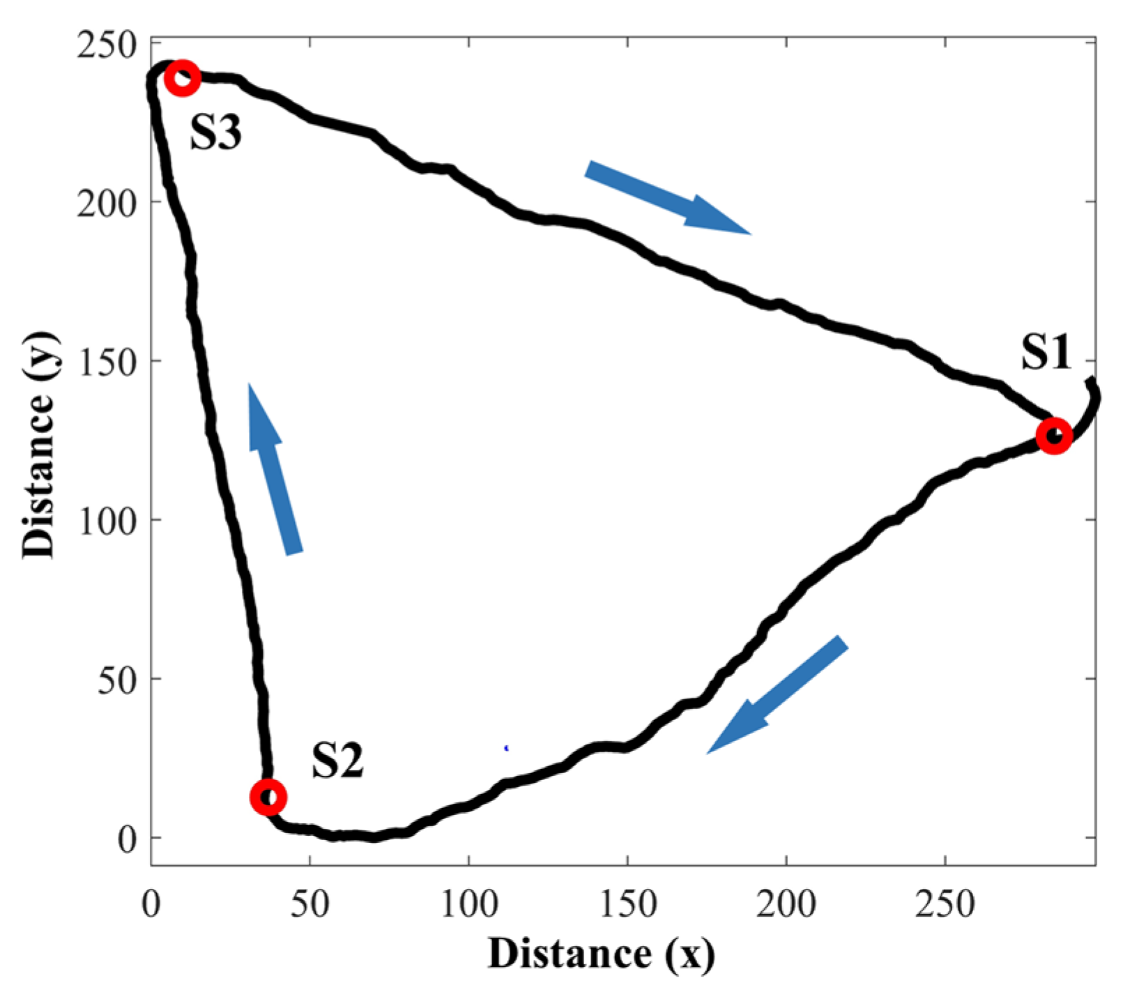
In the experiment, ADCP was navigated along the transmission paths between each pair of stations and followed the route S1→S2→S3→S1 with 1 Hz sampling rate, as shown in Figure 5. Bottom track mode was adopted to collect the topographic data. However, the bottom track mode was only performed once during the experiment. Therefore, depths along station-to-station paths were calculated by the interpolation of topographic data.
3.2. Ray Tracing
The temperature profile measured by TD is shown in Figure 6d. In this section, depth means distance from the surface. The surface temperature was 27.32 °C and the temperature changed slightly at the depth range of 0–9 m. At the depth of about 10 m, there was a sudden temperature change. As depth increased, the temperature decreased nearly linearly. From 30 m, the temperature decreased rapidly and reached 13.81 °C at the depth of 32.47 m.
In Figure 6, with the help of TD and ADCP data (topography), multiple different acoustic ray paths along the vertical slice between stations could be obtained by ray simulation. The SNR of rays reflected more than twice was too low to be identified in cross-correlation results. Therefore, the black dashed rays were deleted, as shown in Figure 6a–c. Finally, three rays, named direct rays (D), surface-reflected rays (S), and bottom-reflected rays (B), respectively, were selected.
The vertical slice was divided into three layers: first layer (0–15 m), second layer (15–25 m), and third layer (below 25 m), respectively. The reference travel time and lengths of each ray could be determined by ray simulation, as shown in Table 2.
Meanwhile, section dividing lines along the horizontal direction were adopted to expand the three layers into nine grids, which were used in 2D vertical slice inversion. For example, at S1–S2, the first layering line along the horizontal direction was 100 m, while the second was 200 m. Table 3 shows the length of rays in each grid and the reference travel time of each ray.
4. Signal Processing and Results
4.1. Multi-Peak Identification
As discussed in Section 2, multi-path sound wave propagation time is a key point for the inversion problem in acoustic tomography research. The quality and dimension of observation results are determined by the quantity and quality of sound wave travel times. In this paper, there are three steps to identify the multi-arrival peaks, which are summarized as follows:
Step 1: Select the rays that need to be identified. Compare the results of ray simulation and the cross-correlation result, and determine the number and structure of potential peaks.
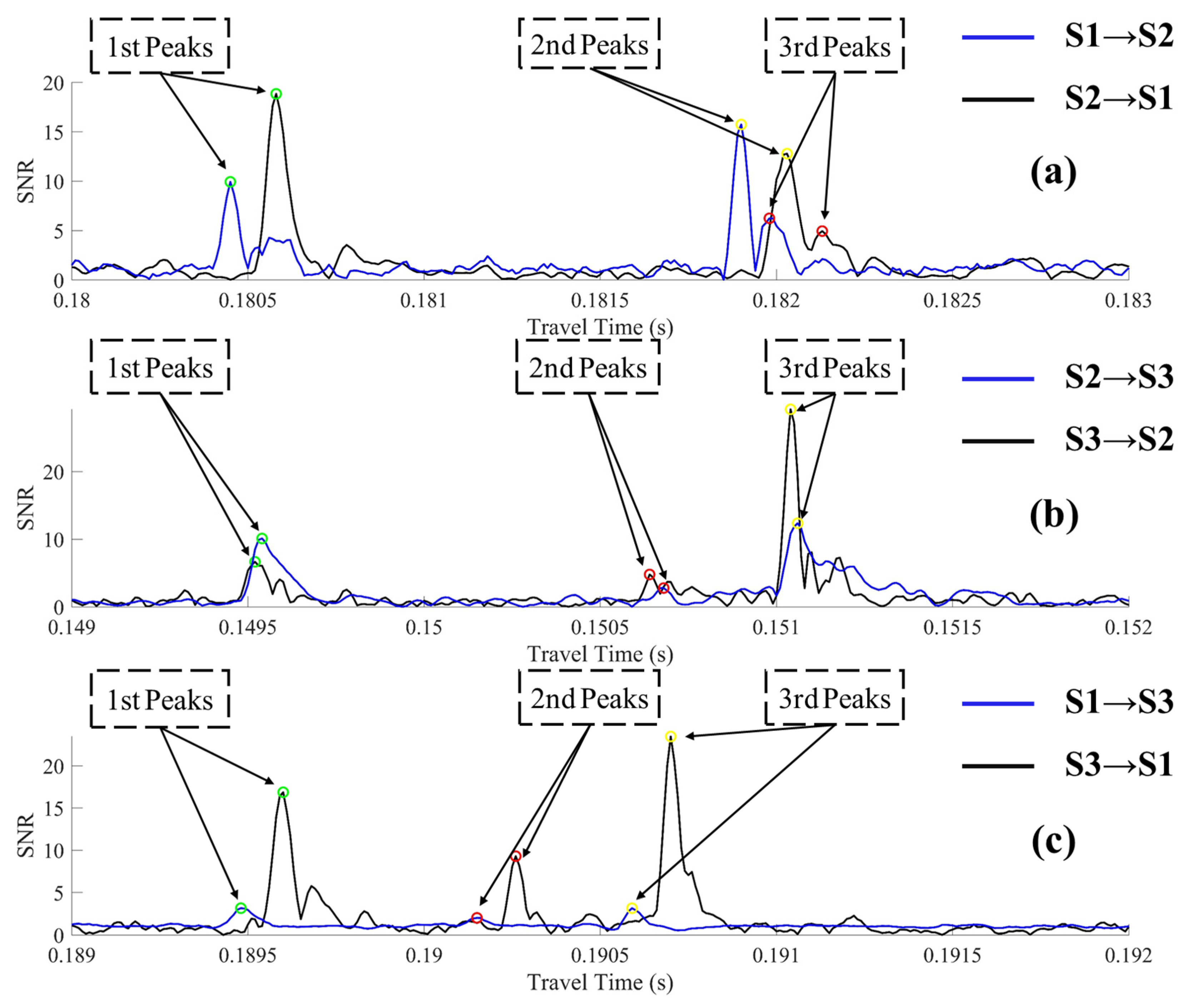
Step 2: Find the first peak: The first peak is generally the direct ray path in small-scale experiments. A 100 ms time window is created to catch the direct peak where the reference travel time obtained from ray simulation is used to locate the position of the time window. The largest peak with SNR greater than 2 is selected as the arrival peak of the direct ray path.
Step 3: Find the second and third peaks: The second and third time windows are also determined by similar processes, where the first arrival signal serves as the standard to locate the latter peaks. The highest SNR peak is found in the respective time windows. Note that because the reference travel time of the second and third peaks in S1–S2 are close, the highest two peaks are found in the same time window. The final travel times are sorted and assigned to the second and third peaks, respectively.
The peak identification results at a particular time during the experiment are shown in Figure 7. In Table 4, the reference travel time obtained from ray simulation and the travel time collected from the arrival peaks in Figure 7 are listed.
The cross-correlation results and multi-peak identifications during the experiment are stacked in Figure 8. The left side shows the colormaps of top-view data, and the magnified figures on the right side are the overlooks of stacked cross-correlation data. The green, yellow, and red circles mark the peaks of the direct path, surface-reflected path, and bottom-reflected path, respectively (from 00:00 to 03:00 on 16 September).
The following can be seen in the colormap in Figure 8: (1) The first and second peaks remained basically unchanged, while the travel time corresponding to the third peak gradually increased, indicating that the rain in the observed area started at 03:00 on 16 September. (2) In Figure 8c, the SNRs of cross-correlation results from S3 to S1 are significantly lower than others, which may have been caused by some unknown environmental fluctuations. (3) Generally speaking, the SNR of the first peak should be the highest, like the correlation results in Figure 8a. However, the third peaks of S2–S3 have the largest SNR. It is speculated that the direct-path sound ray transmission in S2–S3 was affected by the environment. (4) From the magnified results in Figure 8, the SNR of the bottom-reflected paths (red circle) was the lowest due to sound scattering at the fluid–sediment interface [1].
4.2. Inverted Water Temperature Profiling
4.2.1. Travel Time Deviation Preprocessing
Figure 9 shows the travel time deviations of different acoustic rays between each pair of sound stations. The mean and standard travel time deviations are displayed in Table 5. The travel time deviations are calculated by Equation (2).
As shown in Figure 9, the variation trends of three peaks at each pair of stations are basically the same. In Figure 9c, the travel time deviations of S3–S1 fluctuate obviously, corresponding to the low SNR from S3 to S1 in Figure 8c. Furthermore, the average deviations of the third peak between S2–S3 and S3–S1 are significantly higher than others, which means that there were higher temperature fluctuations in the first layer along the S2–S3 path and the S3–S1 path.
4.2.2. Layer-Averaged Water Temperature
The water temperature of different layers and corresponding errors on the vertical slices are shown in Figure 10. The blue lines in Figure 10a–c show the results using the 1 h weighted moving average, which reduces the influence of outliers and retains more changing information through weighting assignment, making the trends of temperature changes more visible.
As shown in Figure 10a–c, the temperature of the first layer decreased during the experiment, which corresponded to a rain event during the experiment. As a contrast, the temperatures of the third layer fluctuated greatly during the experiment, which was caused by the bottom flow. Furthermore, the temperatures of the second layer showed the smallest fluctuations during the observation period.
The right side of Figure 10 shows the inversion errors of the layer method. On the whole, the inversion errors are acceptable for all layers along different slices. The largest inversion errors along different slices are 0.05, 0.065, and 0.21 °C, respectively. The third layers have the largest errors, which results from the smallest layer length in the third layer. The errors of the third layer from S1 to S3 are several times larger than those of the other two paths, resulting from the low SNR value of the cross-correlation peaks.
In brief, the inversion errors are acceptable, indicating the accuracy and reliability of the results.
4.2.3. Two-Dimensional Grid Inversion Method
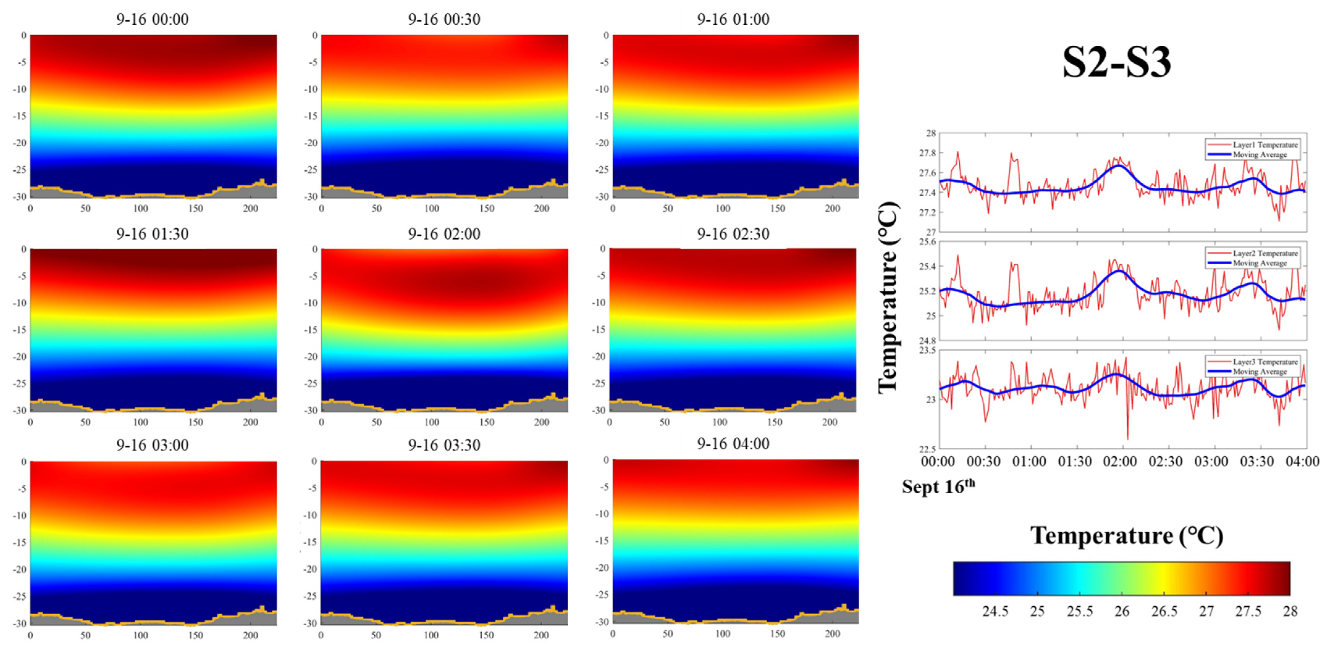
Water temperature variation during the experiment in three vertical slices was also reconstructed with the grid inversion method. Figure 11, Figure 12 and Figure 13 show the 2D vertical temperature fields and corresponding layer-average water temperature between stations S1 and S2. To be concise, we only show the results with an interval of 30 min from 00:00 to 04:00 on 16 September.
As shown in these three figures, the water temperature in the reservoir was horizontally layered, and is affected by the solar energy absorption of water. The water temperature along the vertical slice varied slightly, which may be the result of small-scale dynamic processes and water exchange. The water temperature distribution in a horizontal slice can give a more intuitive picture of water flow.
To conclude, the 2D vertical temperature field is proved to be more intuitive than the layer results to display the distributions and trends of different positions during the observation period.
4.3. Comparison of Inversion Results
The layer-averaged method along a vertical slice has been verified and applied by previous research [1,4,14,17,18]. In order to verify the reliability of the two-dimensional grid inversion method, the average water temperature in each layer obtained by the grid method was calculated and compared with the layer-average temperature obtained from the layer-averaged method. The results are shown in Figure 14 and the RMSEs of each layer between the two methods are shown in Table 6.
The RMSEs between two methods are within 0.1 °C, which is low enough to prove the reliability and accuracy of the grid method. The RMSEs of the second layer are the lowest because the most information of rays is located in the second layer. Similarly, the largest errors of the third layer are caused by the lack of ray information. To further improve the resolution of the water temperature along a vertical slice, a sufficient multi-path sound wave is needed. Abundant arrival sound wave makes the 3D mapping of dynamic processes and water parameters possible.
5. Conclusions
In this paper, a method to reconstruct two-dimensional temperature fields along a vertical slice is proposed, where water temperature profiles can be monitored continuously with only two sound stations. A small-scale CAT observation experiment was carried out in a reservoir with station-to-station distances within 300 m to verify the performance of this new method. Small-scale water temperature fluctuations were obtained in the environment using this two-dimensional grid method. High-quality acoustic rays that penetrate and cover the entire medium were obtained. The vertical water temperature fields between each pair of sound stations were mapped. The accuracy and reliability of this method were proved by comparison with layer-averaged results.
The main conclusions of this research are as follows:
- The quality of the 2D vertical water temperature field is highly dependent on the number of sound rays that are identified. Although obvious multi-arrival ray paths can be identified from the cross-correlation of received acoustic data, it is difficult to match the ray simulation results with the real multi-arrival signal peaks. Consequently, two important factors of high-quality data are: (1) adequate arrival peaks of cross-correlation data, and (2) accurate topographic data of the experimental areas.
- A two-dimensional vertical water temperature field can be successfully established by the grid method with sound waves. The 2D vertical water temperature field is more intuitive than the layer-averaged results in displaying the distributions and trends of different positions during the observation period.
- By error analysis and comparison with the layer-averaged method, the method proposed in this paper is proved to be of high accuracy to profile the vertical temperature field along a vertical slice.
3D water temperature field observations can be conducted with this method in future research by combining the analysis of water temperature in a horizontal slice. High-resolution sensing results of water processes can be acquired using a multi-station sensing network.
Author Contributions
Conceptualization, H.H., X.X., Y.G. and G.L.; funding acquisition, H.H., L.M. and G.L.; experiments, X.X., Y.G., G.L. and S.X.; method, X.X., Y.G., G.L. and S.X.; data analysis, X.X., Y.G., G.L. and S.X.; writing, X.X., Y.G., G.L. and S.X. All authors have read and agreed to the published version of the manuscript.
Funding
This research was funded by the National Science Foundation of China (grant numbers 52071293 and 51809274).
Institutional Review Board Statement
Not applicable.
Informed Consent Statement
Not applicable.
Data Availability Statement
The data presented in this study are available on request from the underwater acoustic tomography group (E-mail: [email protected]).
Acknowledgments
Pan Xu, Bingbing Zhang, Zhengliang Hu, and Min Zhu from the National University of Defense Technology provided valuable support for this experiment. The authors are appreciated for their suggestions of guest editors and reviewers, which helped to improve of this paper and get it published successfully.
Conflicts of Interest
The authors declare no conflict of interest.
References
- Kaneko, A.; Zhu, X.; Lin, J. Coastal Acoustic Tomography; Academic Press: Cambridge, MA, USA; Elsevier: Amsterdam, The Netherlands, 2020. [Google Scholar]
- Anas, A.; Krishna, K.; Vijayakumar, S.; George, G.; Menon, N.; Kulk, G.; Chekidhenkuzhiyil, J.; Ciambelli, A.; Kuttiyilmemuriyil Vikraman, H.; Tharakan, B.; et al. Dynamics of Vibrio cholerae in a Typical Tropical Lake and Estuarine System: Potential of Remote Sensing for Risk Mapping. Remote Sens. 2021, 13, 1034. [Google Scholar] [CrossRef]
- Hidalgo Garcia, D.; Arco Diaz, J. Spatial and Multi-Temporal Analysis of Land Surface Temperature through Landsat 8 Images: Comparison of Algorithms in a Highly Polluted City (Granada). Remote Sens. 2021, 13, 1012. [Google Scholar] [CrossRef]
- Syamsudin, F.; Chen, M.; Kaneko, A.; Adityawarman, Y.; Zheng, H.; Mutsuda, H.; Hanifa, A.D.; Zhang, C.; Auger, G.; Wells, J.C.; et al. Profiling measurement of internal tides in Bali Strait by reciprocal sound transmission. Acoust. Sci. Technol. 2017, 38, 246–253. [Google Scholar] [CrossRef]
- Wang, L.; Wang, Y.; Wang, J.; Li, F. A High Spatial Resolution FBG Sensor Array for Measuring Ocean Temperature and Depth. Photonic Sens. 2020, 10, 57–66. [Google Scholar] [CrossRef] [Green Version]
- Munk, W.; Wunsch, C. Ocean acoustic tomography—Scheme for large-scale monitoring. Deep Sea Res. Part A Oceanogr. Res. Pap. 1979, 26, 123–161. [Google Scholar] [CrossRef]
- Munk, W.; Worceser, P.F.; Wunsch, C. Ocean Acoustic Tomography; Cambridge Univ. Press: New York, NY, USA, 1995; p. 433. [Google Scholar]
- Duda, T.F.; Flatte, S.M.; Colosi, J.A.; Cornuelle, B.D.; Hildebrand, J.A.; Hodgkiss, W.S.; Worcester, P.F.; Howe, B.M.; Mercer, J.A.; Spindel, R.C. Measured wave-front fluctuations in 1000-km pulse-propagation in the pacific-ocean. J. Acoust. Soc. Am. 1992, 92, 939–955. [Google Scholar] [CrossRef]
- Skarsoulis, E.K.; Athanassoulis, G.A.; Send, U. Ocean acoustic tomography based on peak arrivals. J. Acoust. Soc. Am. 1996, 100, 797–813. [Google Scholar] [CrossRef]
- Hong, Z.; Haruhiko, Y.; Noriaki, G.; Hideaki, N.; Arata, K. Design of the acoustic tomography system for velocity measurement with an application to the coastal sea. Acoust. Soc. Jpn. 1998, 19, 199–210. [Google Scholar]
- Zhang, C.; Kaneko, A.; Zhu, X.-H.; Gohda, N. Tomographic mapping of a coastal upwelling and the associated diurnal internal tides in Hiroshima Bay, Japan. J. Geophys. Res. Ocean. 2015, 120, 4288–4305. [Google Scholar] [CrossRef]
- Zhang, C.; Kaneko, A.; Zhu, X.-H.; Howe, B.M.; Gohda, N. Acoustic measurement of the net transport through the Seto Inland Sea. Acoust. Sci. Technol. 2016, 37, 10–20. [Google Scholar] [CrossRef]
- Huang, H.; Guo, Y.; Wang, Z.; Shen, Y.; Wei, Y. Water Temperature Observation by Coastal Acoustic Tomography in Artificial Upwelling Area. Sensors 2019, 19, 2655. [Google Scholar] [CrossRef] [Green Version]
- Huang, H.; Guo, Y.; Li, G.; Arata, K.; Xie, X.; Xu, P. Short-Range Water Temperature Profiling in a Lake with Coastal Acoustic Tomography. Sensors 2020, 20, 4498. [Google Scholar] [CrossRef]
- Roux, P.; Cornuelle, B.D.; Kuperman, W.A.; Hodgkiss, W.S. The structure of raylike arrivals in a shallow-water waveguide. J. Acoust. Soc. Am. 2008, 124, 3430–3439. [Google Scholar] [CrossRef]
- Elisseeff, P.; Schmidt, H.; Johnson, M.; Herold, D.; Chapman, N.R.; McDonald, M.M. Acoustic tomography of a coastal front in Haro Strait, British Columbia. J. Acoust. Soc. Am. 1999, 106, 169–184. [Google Scholar] [CrossRef]
- Luo, J.; Karjadi, E.A.; Badiey, M. High-frequency broadband acoustic current tomography in shallow water. J. Acoust. Soc. Am. 2008, 123, 3914. [Google Scholar] [CrossRef]
- Li, G.; Ingram, D.; Kaneko, A.; Chen, M.; Gohda, N.; Polydorides, N. Vertical underwater acoustic tomography in an experimental basin. J. Acoust. Soc. Am. 2017, 141, 3656. [Google Scholar] [CrossRef]
- Yu, X.; Zhuang, X.; Li, Y.; Zhang, Y. Real-Time Observation of Range-Averaged Temperature by High-Frequency Underwater Acoustic Thermometry. IEEE Access 2019, 7, 17975–17980. [Google Scholar] [CrossRef]
- Huang, C.-F.; Chen, K.; Huang, S.-W.; Guo, J.; Taniguchi, N. Acoustic mapping of ocean currents using moving vehicles. J. Acoust. Soc. Am. 2018, 144, 1982. [Google Scholar] [CrossRef]
- Huang, C.-F.; Li, Y.-W.; Taniguchi, N. Mapping of ocean currents in shallow water using moving ship acoustic tomography. J. Acoust. Soc. Am. 2019, 145, 858–868. [Google Scholar] [CrossRef] [PubMed]
- Chen, K.; Huang, C.-F.; Huang, S.-W.; Liu, J.-Y.; Guo, J. Mapping coastal circulations using moving vehicle acoustic tomography. J. Acoust. Soc. Am. 2020, 148, EL353–EL358. [Google Scholar] [CrossRef]
- Carriere, O.; Hermand, J.-P. Feature-Oriented Acoustic Tomography for Coastal Ocean Observatories. IEEE J. Ocean. Eng. 2013, 38, 534–546. [Google Scholar] [CrossRef]
- Syamsudin, F.; Taniguchi, N.; Zhang, C.; Hanifa, A.D.; Li, G.; Chen, M.; Mutsuda, H.; Zhu, Z.-N.; Zhu, X.-H.; Nagai, T.; et al. Observing Internal Solitary Waves in the Lombok Strait by Coastal Acoustic Tomography. Geophys. Res. Lett. 2019, 46, 10475–10483. [Google Scholar] [CrossRef] [Green Version]
- Liu, W.; Zhu, X.; Zhu, Z.; Fan, X.; Dong, M.; Zhang, Z. A Coastal Acoustic Tomography Experiment in the Qiongzhou Strait; IEEE: Piscataway, NJ, USA, 2016. [Google Scholar]
- Mackenzie, K.V. Nine-term equation for sound speed in the oceans. J. Acoust. Soc. Am. 1981, 70, 807–812. [Google Scholar] [CrossRef]
Figure 1.
Sound propagation structure and layer division. Two sound transceivers are deployed in the water and transmit sound reciprocally. Sound waves are reflected by the interface, where multi-path sound propagation is achieved. (a) Sound speed profile. (b) Corresponding acoustic rays.
Figure 1.
Sound propagation structure and layer division. Two sound transceivers are deployed in the water and transmit sound reciprocally. Sound waves are reflected by the interface, where multi-path sound propagation is achieved. (a) Sound speed profile. (b) Corresponding acoustic rays.

Figure 2.
The vertical grid division. The vertical slice is divided into different grids, sound rays propagate across the grids, and water parameter information is taken away. More unknown parameters are introduced in this case.
Figure 2.
The vertical grid division. The vertical slice is divided into different grids, sound rays propagate across the grids, and water parameter information is taken away. More unknown parameters are introduced in this case.

Figure 3.
The left figure shows a map of the Huangcai Reservoir and adjacent regions. The southeast part of Huangcai Reservoir is magnified in the right figure, which shows the position of CAT stations (S1, S2, S3), the point of the TD, and the routes of ADCP sailings. The green solid lines are the projection of acoustic ray paths in the horizontal slice. The upper-right corner of the magnified figure is a photo of the CAT system used at station S1.

Figure 4.
Layout of the three sound stations, including anchored ships, floating balls, additional weights, and CAT systems. The depth of the transceivers and the distance between the stations are shown in Table 1.
Figure 4.
Layout of the three sound stations, including anchored ships, floating balls, additional weights, and CAT systems. The depth of the transceivers and the distance between the stations are shown in Table 1.

Figure 5.
Sailing route of the ADCP mounted boat, moving clockwise along the blue arrows.

Figure 6.
(a–c) The results of the ray simulation in three sections; (e–g) the launch angles of corresponding ray paths; (d) the temperature profiling obtained with TD. The white dotted lines in (a–c) divide the vertical slice into nine grids. The red, green, and yellow lines indicate bottom-reflected paths, direct paths, and surface-reflected paths, respectively. The black dotted lines indicate the possible acoustic ray paths, the pink dots indicate the center point of each grid.

Figure 7.
Peak identification of acoustic signal propagated between sound station pairs at a particular time. (a–c) The sound propagation path results of S1–S2, S2–S3 and S3–S1, respectively.
Figure 7.
Peak identification of acoustic signal propagated between sound station pairs at a particular time. (a–c) The sound propagation path results of S1–S2, S2–S3 and S3–S1, respectively.

Figure 8.
Multi-peaks identification. (a–c) The results of peak extraction after S1–S2, S2–S3, and S3–S1 correlation, respectively. The abscissa axis in colormaps is the travel time of signals; the ordinate axis indicates the time at which signals were sent; the color depth value indicates the SNR. The magnified figures are shown as three-dimensional coordinates. The abscissa and ordinate coordinates are the same as the colormap, and the height is the SNR value.


Figure 9.
Travel time deviations. (a–c) The travel time deviations of three peaks between S1–S2, S2–S3, and S3–S1, respectively.
Figure 9.
Travel time deviations. (a–c) The travel time deviations of three peaks between S1–S2, S2–S3, and S3–S1, respectively.

Figure 10.
Layer-averaged water temperature between three sound stations. (a–c) The temperature inversion results of vertical slices between stations (red lines indicate the temperature of each layer (7.5 m, 20 m, 28 m), blue lines indicate the results passing through the 1 h weighted moving average). (d–f) Inversion errors (the red, black, blue lines indicate the first, second, and third layers, respectively.).

Figure 11.
Colormaps of the water temperature field along a vertical slice between stations S1 and S2. The figure on the right shows the temperature of each layer in the corresponding time period intercepted from Figure 10.
Figure 11.
Colormaps of the water temperature field along a vertical slice between stations S1 and S2. The figure on the right shows the temperature of each layer in the corresponding time period intercepted from Figure 10.
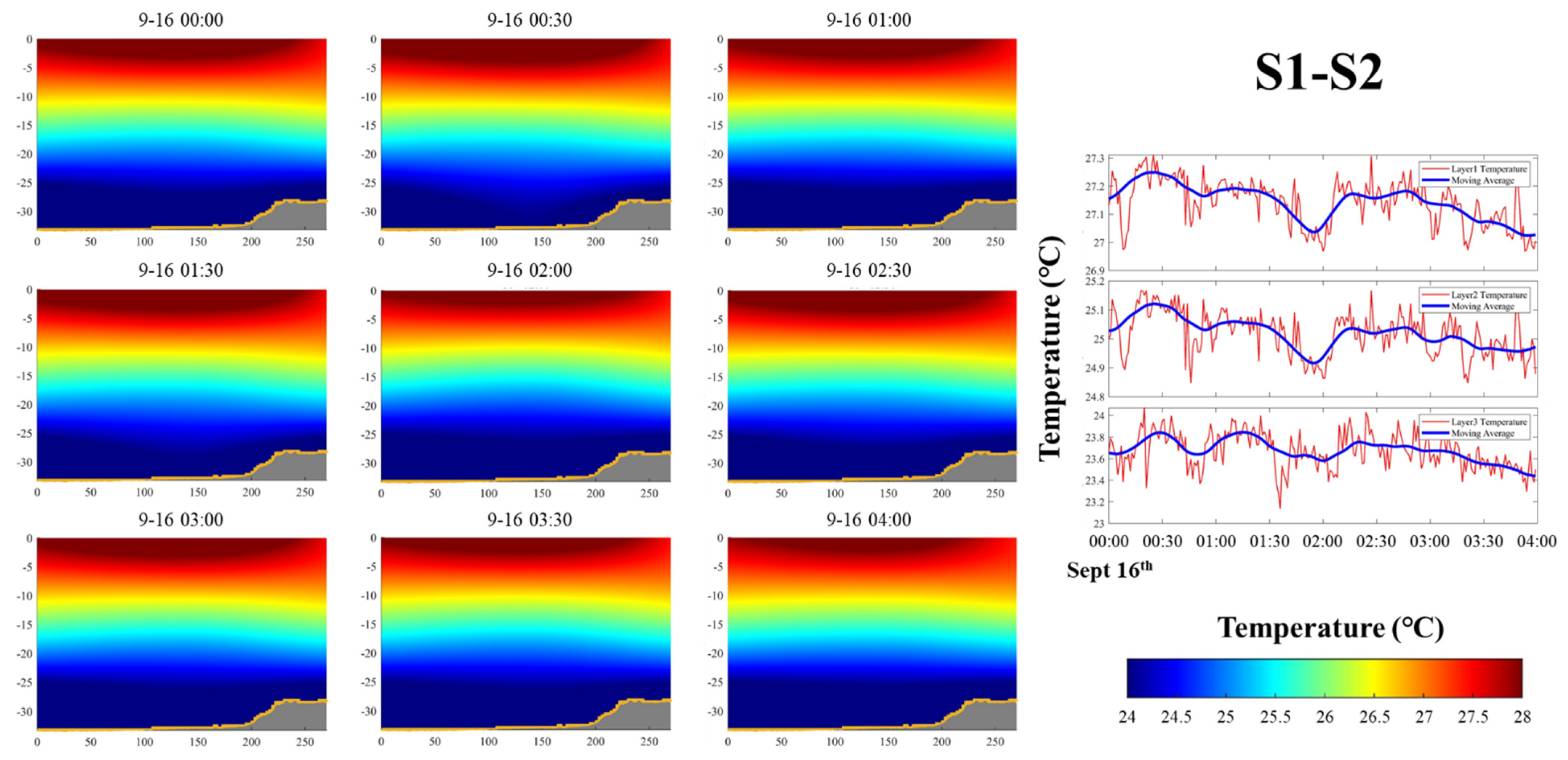
Figure 12.
Colormap of the vertical temperature field between stations S2 and S3. The figure on the right shows the temperatures of each layer in the corresponding time period intercepted from Figure 10.
Figure 12.
Colormap of the vertical temperature field between stations S2 and S3. The figure on the right shows the temperatures of each layer in the corresponding time period intercepted from Figure 10.

Figure 13.
Colormap of the vertical temperature field between stations S3 and S1. The figure on the right shows the temperatures of each layer in the corresponding time period intercepted from Figure 10.
Figure 13.
Colormap of the vertical temperature field between stations S3 and S1. The figure on the right shows the temperatures of each layer in the corresponding time period intercepted from Figure 10.

Figure 14.
Comparison of layer average water temperature. (a–c) The comparison of average temperature curves between the grid method and the layer-averaged method. The red and blue lines indicate the average temperature in each layer obtained by the grid method and the layer-averaged method after a weighted moving average.


Table 1.
Acoustic signal and sound station parameters.
| Item | Value | ||
|---|---|---|---|
| Central frequency (kHz) | 50 | ||
| Order of M sequence | 10 | ||
| Q 1 | 2 | ||
| Transmit interval (min) | 1 | ||
| Start and end date | Sept.15 09:00–Sept.16 16:00 | ||
| Station | S1 | S2 | S3 |
| Station distance (m) 2 | L12 = 270.00 | L23 = 224.01 | L31 = 283.64 |
| Transceiver depth (m) | 20 | 20 | 16.86 |
1 The Q value denotes the number of cycles per digit in the M sequence. 2 L12, L23, and L31 denote the station-to-station distances between S1–S2, S2–S3, and S3–S1, respectively.
Table 2.
Ray length in each layer and reference travel time (three rays and three layers).
| Stations | S1–S2 | S2–S3 | S3–S1 | ||||||
|---|---|---|---|---|---|---|---|---|---|
| Ray Path | D 1 | S 2 | B 3 | D | S | B | D | S | B |
| Layer 1 | 0 | 209.946 | 0 | 0 | 188.490 | 0 | 0 | 238.576 | 0 |
| Layer 2 | 270.068 4 | 272.983 | 142.737 | 224.037 | 38.509 | 139.634 | 283.775 | 47.533 | 249.815 |
| Layer 3 | 0 | 0 | 129.167 | 0 | 0 | 85.523 | 0 | 0 | 34.515 |
| Total 4 (m) | 270.068 | 272.98 | 271.904 | 224.037 | 226.999 | 225.157 | 283.775 | 286.109 | 284.33 |
| TT 5 (s) | 0.18038 | 0.18191 | 0.18217 | 0.14962 | 0.15124 | 0.15061 | 0.18947 | 0.19061 | 0.19010 |
1 D denotes the direct acoustic ray path. 2 S denotes the surface-reflected acoustic ray path. 3 B denotes the bottom-reflected acoustic ray path. 4 Total denotes the distance that is the average of all data at different times. 5 TT denotes the reference travel time of each ray.
Table 3.
Ray length in each grid and reference travel time (three rays and nine grids).
| Stations | S1–S2 | S2–S3 | S3–S1 | ||||||
|---|---|---|---|---|---|---|---|---|---|
| Ray Path | D | S | B | D | S | B | D | S | B |
| Grid 1 | 0 | 70.033 | 0 | 0 | 42.469 | 0 | 0 | 66.249 | 0 |
| Grid 2 | 0 | 100.97 | 0 | 0 | 101.22 | 0 | 0 | 100.73 | 0 |
| Grid 3 | 0 | 38.944 | 0 | 0 | 44.802 | 0 | 0 | 28.498 | 0 |
| Grid 4 | 100.03 | 31.114 | 26.504 | 70.027 | 28.55 | 58.125 | 100.01 | 34.605 | 59.162 |
| Grid 5 | 100.01 | 0 | 46.182 | 100.01 | 0 | 27.246 | 100.01 | 0 | 45.837 |
| Grid 6 | 70.028 | 31.924 | 70.05 | 54 | 9.958 | 54.262 | 83.755 | 56.027 | 83.712 |
| Grid 7 | 0 | 0 | 75.167 | 0 | 0 | 12.147 | 0 | 0 | 44.367 |
| Grid 8 | 0 | 0 | 54.001 | 0 | 0 | 73.377 | 0 | 0 | 54.252 |
| Grid 9 | 0 | 0 | 0 | 0 | 0 | 0 | 0 | 0 | 0 |
| Total (m) | 270.068 | 272.98 | 271.904 | 224.037 | 226.999 | 225.157 | 283.775 | 286.109 | 284.33 |
| TT (s) | 0.18038 | 0.18191 | 0.18217 | 0.14962 | 0.15124 | 0.15061 | 0.18947 | 0.19061 | 0.19010 |
Table 4.
The arrival time of each peak between sound stations (unit: s).
| Peaks | S1→S2 | S2→S1 | S12-RS 1 | |
| 1st Peak | 0.1804 | 0.1805 | 0.18038 | D |
| 2nd Peak | 0.1819 | 0.1820 | 0.18191 | S |
| 3rd Peak | 0.1820 | 0.2821 | 0.18217 | B |
| Peaks | S2→S3 | S3→S2 | S23-RS | |
| 1st Peak | 0.1495 | 0.1496 | 0.14962 | D |
| 2nd Peak | 0.1506 | 0.1507 | 0.15061 | B |
| 3rd Peak | 0.1510 | 0.1511 | 0.15124 | S |
| Peaks | S1→S3 | S3→S1 | S13-RS | |
| 1st Peak | 0.1895 | 0.1896 | 0.18947 | D |
| 2nd Peak | 0.1902 | 0.1903 | 0.19010 | B |
| 3rd Peak | 0.1906 | 0.1907 | 0.19061 | S |
1 RS denotes reference travel time calculated by ray simulation.
Table 5.
Mean and standard deviation of travel time deviations.
| Stations | S1–S2 | S2–S3 | S3–S1 | ||||||
|---|---|---|---|---|---|---|---|---|---|
| Peaks | 1st Peak | 2nd Peak | 3rd Peak | 1st Peak | 2nd Peak | 3rd Peak | 1st Peak | 2nd Peak | 3rd Peak |
| Terr-M 1 | 0.0097 | 0.0164 | 0.0496 | 0.0019 | 0.0114 | 0.0652 | 0.0037 | 0.0114 | 0.1677 |
| Terr-S 2 | 0.0013 | 0.0005 | 0.0008 | 0.0013 | 0.0142 | 0.1677 | 0.0031 | 0.0026 | 0.0456 |
1 Mean of travel time deviation. 2 Standard deviation of travel time deviation.
Table 6.
RMSEs of the comparison of the average water temperature in each layer obtained by the grid method and the layer-averaged method.
Table 6.
RMSEs of the comparison of the average water temperature in each layer obtained by the grid method and the layer-averaged method.
| RMSE (°C) 1 | S1–S2 | S2–S3 | S3–S1 |
|---|---|---|---|
| Layer 1 | 0.0122 | 0.0359 | 0.0073 |
| Layer 2 | 0.0042 | 0.0084 | 0.0082 |
| Layer 3 | 0.0963 | 0.0873 | 0.0712 |
1 Root-mean-square error of temperature.
Publisher’s Note: MDPI stays neutral with regard to jurisdictional claims in published maps and institutional affiliations. |
© 2021 by the authors. Licensee MDPI, Basel, Switzerland. This article is an open access article distributed under the terms and conditions of the Creative Commons Attribution (CC BY) license (https://creativecommons.org/licenses/by/4.0/).
Share and Cite
MDPI and ACS Style
Huang, H.; Xu, S.; Xie, X.; Guo, Y.; Meng, L.; Li, G. Continuous Sensing of Water Temperature in a Reservoir with Grid Inversion Method Based on Acoustic Tomography System. Remote Sens. 2021, 13, 2633. https://doi.org/10.3390/rs13132633
AMA Style
Huang H, Xu S, Xie X, Guo Y, Meng L, Li G. Continuous Sensing of Water Temperature in a Reservoir with Grid Inversion Method Based on Acoustic Tomography System. Remote Sensing. 2021; 13(13):2633. https://doi.org/10.3390/rs13132633
Chicago/Turabian StyleHuang, Haocai, Shijie Xu, Xinyi Xie, Yong Guo, Luwen Meng, and Guangming Li. 2021. "Continuous Sensing of Water Temperature in a Reservoir with Grid Inversion Method Based on Acoustic Tomography System" Remote Sensing 13, no. 13: 2633. https://doi.org/10.3390/rs13132633
Note that from the first issue of 2016, this journal uses article numbers instead of page numbers. See further details here.