Effects of Cloud Microphysics on the Vertical Structures of Cloud Radiative Effects over the Tibetan Plateau and the Arctic

Abstract

The Tibetan Plateau (TP) and the Arctic are both cold, fragile, and sensitive to global warming. However, they have very different cloud radiative effects (CRE) and influences on the climate system. In this study, the effects of cloud microphysics on the vertical structures of CRE over the two regions are analyzed and compared by using CloudSat/CALIPSO satellite data and the Rapid Radiative Transfer Model. Results show there is a greater amount of cloud water particles with larger sizes over the TP than over the Arctic, and the supercooled water is found to be more prone to exist over the former than the latter, making shortwave and longwave CRE, as well as the net CRE, much stronger over the TP. Further investigations indicate that the vertical structures of CRE at high altitudes are primarily dominated by cloud ice water, while those at low altitudes are dominated by cloud liquid and mixed-phase water. The liquid and mixed-phase water results in a strong shallow heating (cooling) layer above the cooling (heating) layer in the shortwave (longwave) CRE profiles, respectively.

1. Introduction

Clouds have a crucial effect on the radiation budget of the Earth via the reflection of shortwave (SW) and absorption of longwave (LW) radiation by both ice and liquid water particles in clouds [1,2]. The balance of these SW and LW effects is referred to as cloud radiative effects (CRE), with positive values indicating that clouds warm the surface/atmosphere/Earth relative to clear sky conditions and negative values indicating that clouds cool the surface/atmosphere/Earth. Studies have found that cloud radiation characteristics are closely related to cloud phase and cloud microphysical properties [3,4]. Due to the lack of knowledge concerning cloud vertical structures and their microphysical processes, clouds remain one of the largest sources of uncertainty in climate model simulations [5,6,7] and the precise modeling of cloud–radiation interactions remains uncertain. Investigating the vertical microphysical characteristics of clouds and CRE for a variety of conditions and locations is important to determine the dynamics of the general circulation, as well as to improve the simulation performance of climate models, therefore promoting climate research processes.

The Tibetan Plateau (TP) and the Arctic are fragile regions that are sensitive to global warming [8,9].

The TP, often referred to as the third pole of the Earth, has the highest mountain on Earth and significantly affects atmospheric circulation and the Asian climate [10,11,12,13]. Despite numerous studies analyzing cloud microphysical or macrophysical properties over the TP [14,15,16,17,18,19,20,21,22], interest in CRE over the TP is rare and a few studies focus on CRE on the ground surface of Earth system. For example, the surface irradiation over the TP has been found to be higher than that over other areas at the same latitude and can frequently exceed the solar constant because of multiple scattering in clouds over the plateau [23,24]. The CRE over the TP has been found to be dominated by cooling effects [25], and the downward SW flux over the TP is modulated by cloud cover and the cloud optical thickness [26]. Nevertheless, the vertical structures of CRE in the atmosphere, which directly affect the atmospheric circulation, are rarely mentioned because of the lack of direct observations. Yan et al. [19] demonstrated that the TP has a unique vertical structure of atmospheric CRE compared with neighboring regions, especially with respect to the existence of a strong cooling layer of net CRE at an altitude of 8 km in boreal summer, according to products from CloudSat/CALIPSO satellites. However, it is urgent to answer the following question: what causes the unique atmospheric CRE over the TP? An appropriate answer to this question is essential to accurately understand the interactions between cloud, precipitation, radiation, and large-scale circulation over the plateau.

The Arctic is another sensitive area of climate change in the Northern Hemisphere, and the cloud–radiation feedback there is believed to play an important role in the Arctic climate system [27]. By modulating the LW and SW radiant fluxes, Arctic clouds are crucial for determining the energy balance at the top of the atmosphere and surface [28,29], which may regulate the growth or withdrawal of the sea ice range and thickness via effects on the surface temperature [30,31]. For example, extreme poleward transport of water vapor caused by global warming, on one hand, accelerates the melting of sea ice in the Arctic through the influence of LW radiation on the surface; on the other hand, it leads to additional cloud radiative heating through increased vertical cloudiness [32]. However, the retreat of the sea ice coverage can further lead to changes in the cloud amount and cloud vertical structures [33,34]. A recent study found that the cloud cover over the Arctic has been increasing in October with an approximate 1 month lag behind the sea ice reduction, which may result in further sea ice retreat and enhance the feedback processes of Arctic warming [35]. Earlier studies [36,37] suggested that infrared radiation emitted from clouds toward the surface can cause sea ice melting and that the cloud phase may be related to anomalies in the downward LW radiation. Overall, there are complex interactions between clouds and other processes in the Arctic climate system and an accurate description of the cloud microphysical properties and their radiative effects are important to understand these interactions. Furthermore, considerable differences exist between atmospheric climate models in terms of cloud-related variables, such as surface downwelling solar and terrestrial radiation, surface albedo, vertically integrated water vapor, liquid water paths, and cloud cover [38,39,40]. Therefore, improvements in the parameterization of clouds are urgently needed to improve the overall performance of climate models in the Arctic. Even though a large amount of attention has been given to the study of cloud properties and the CRE on top of the atmosphere or surface in the Arctic [36,41,42,43,44,45,46,47,48], similar to the TP, fewer studies have focused on the vertical structures of CRE, which have a direct effect on atmospheric circulation. Accordingly, we pose the following question: what is the vertical distribution of CRE in the atmosphere over the Arctic?

Recently, while focused on mixed-phase clouds, we found that abundant mixed-phase clouds exist over these two regions and that the atmospheric heating profile induced by mixed-phase clouds exhibits larger vertical contrasts and more seasonal variations over the TP than over the Arctic [49]. However, the differences in the general atmospheric heating profiles (induced by general clouds, including not only mixed-phase clouds but also pure ice or pure liquid clouds), as well as the relationships between the vertical structures of the clouds and the cloud microphysical properties, remain unclear.

In this study, we aim to reveal the comparative vertical structures of CRE and related cloud microphysical characteristics over the TP and the Arctic based on CloudSat/CALIPSO products. Then, we will investigate the effects of cloud microphysical characteristics on the vertical distribution of CRE over both regions. The definition of the TP area (latitude: 27–40° N, longitude: 70–103° E, altitude: >3000 m) is consistent with Yan et al. [19,20,21,49]. As the maximum latitudinal coverage of the CloudSat/CALIPSO polar-orbiting satellites is near ±80°, the Arctic region is defined as the annular zonal area between 72.5° N and 77.5° N, which is consistent with Yan et al. [49].

This paper is organized as follows. Section 2 covers the data and methodology. Section 3 presents results concerning the vertical distribution of the cloud microphysics properties and CRE, as well as the contributions of cloud microphysics in terms of different water phases on the vertical structures of CRE. Section 4 presents our conclusions and a discussion.

2. Data and Methodology

2.1. Data

The CloudSat [50] and CALIPSO [51] satellites, flying in a close sun-synchronous near-polar orbit at approximately 705 km above the Earth’s surface and overpassing the equator at approximately 01:30 and 13:30 local time, were launched in 2006 as part of the NASA A-Train constellation of satellites. Their mission is to measure cloud internal properties and vertical structures from space based on active sensors. The millimeter-wavelength Cloud Profiling Radar onboard the CloudSat satellite is a 94-GHz nadir-viewing radar measuring the backscattered power resulting from clouds and precipitation particles in the atmospheric column within a 1.4 km across-track by 2.5 km along-track radar footprint. The Cloud Profiling Radar has great advantages when optically probing thick large-particle layers, while the Cloud-Aerosol Lidar with Orthogonal Polarization onboard the CALIPSO satellite can sense optically thin layers and tenuous cloud tops. The combination of the two provides an unprecedented opportunity to explore cloud internal vertical properties based on active sensors.

The primary datasets used for this study were 2B-CWC-RO [52,53] and 2B-FLXHR-LIDAR [54,55,56] (both version r04) estimated from the CloudSat/CALIPSO satellites. To obtain robust conclusions, we chose datasets with the same period from 6 July 2006 to 17 April 2011. A brief introduction to each dataset is given here, and more detailed information concerning the products can be found online (http://www.cloudsat.cira.colostate.edu/data-products/level-2b. Accessed on 23 April 2020).

The 2B-CWC-RO product contains the retrieved cloud liquid and ice water content, particle effective radius, and number concentration estimated from a calibrated radar reflectivity factor converted from measurements of the radar backscatter for each CloudSat profile. Retrievals for the liquid and ice phases are performed separately and primarily depend on the temperature. The two resultant profiles are then combined into a composite profile that is consistent with the input measurements. The cloud liquid water estimates are obtained only in the portion of the profile warmer than 0 °C, the cloud ice water estimates are obtained only in the portion of the profile colder than −20 °C, and a linear combination of the two is obtained in the intermediate temperature range [52]. The cloud radar can accurately sense between −28 and 6 dBZe and can sense above 6 dBZe with an error of ±50% [57]. As CloudSat cannot accurately retrieve clouds in the lowest 1 km near the surface, we limited our analysis to cloud profiles above 1 km.

The 2B-FLXHR-LIDAR product provides the upwelling and downwelling LW and SW fluxes of each profile, as well as the heating rates inferred from these fluxes at discrete levels in the atmosphere. It makes use of the liquid and ice water contents estimated from the Cloud Profiling Radar and additional cloud and aerosol properties detected by CALIPSO and MODIS (the Moderate Resolution Imaging Spectroradiometer), combined with the atmospheric profiles from ECMWF reanalysis. The FLXHR radiative transfer algorithms perform independent flux calculations over 12 LW bands and 6 solar bands that are ultimately combined into 2 broadband (SW bands: wavelengths greater than 0.2 µm and less than 4.0 µm; LW bands: wavelengths greater than 4.55 µm) flux estimates with vertical resolutions of ~240 m. For the SW bands, molecular (Rayleigh) scattering and condensed water optical properties are treated as gray properties. Refractive effects are considered in the visible bands. For the LW bands, the condensed water optics is considered grey along with the water vapor continuum absorption and Planck emissions [55]. Using a “status flag” (a value between 1 and 20), the 2B-FLXHR-LIDAR product identifies the cloud type or types present in the scene for each pixel and indicates scenes that may be contaminated with drizzle. Pixels with a status flag value of 8 or less contain valid flux and heating rate output; this is also the criterion for valid data adopted in the diagnostics. The atmospheric fluxes and heating rates are accurate to 5 W m⁻² and 1 K day⁻¹, respectively, at a resolution of 500 m [55].

In this study, we first converted the CloudSat/CALIPSO products from the original orbital data to daily grid data with a horizontal resolution of 2.5° × 2.5° and a vertical resolution of 240 m, wherein the cloud properties for each lattice are the average of all the pixels passing through the grid box, such that there is only one value for each grid representing the average properties within a meridional or zonal extent of ± 1.25°. The average daily number of valid climatology samples for each grid cell is approximately 280 granules during the 5 years of data, and the global sample distribution is basically uniform [19]. The daily climatological grid data of CloudSat/CALIPSO were used to analyze the regional averages of the cloud properties and as input of the Rapid Radiative Transfer Model (RRTM).

2.2. The Rapid Radiative Transfer Model (RRTM)

The accurate and rapid radiative transfer model RRTM (Version 3.3) used for the calculation of the LW and SW atmospheric radiative fluxes and heating rates was developed by Mlawer et al. [58] and has been widely used since then [59]. A key aspect of RRTM is the correlated-k method, which is an accurate and computationally fast radiative transfer scheme that greatly reduces the radiative transfer computation time. The k-distribution coefficient needed by RRTM is generated using the Line-By-Line Radiative Transfer Model, and its calculation accuracy agrees with the Line-By-Line Radiative Transfer Model within ~1 W m⁻² for the LW fluxes and ~1.5 W m⁻² for the SW fluxes [60,61].

For the LW radiation scheme in RRTM, the fluxes and heating rates are calculated in 16 contiguous bands with spectrum ranges from 10 to 3250 cm⁻¹. To perform a comparison with the values from 2B-FLXHR-LIDAR, we only selected bands whose spectrum ranged between 10 and 2250 cm⁻¹ (corresponding to the LW spectrum greater than 4.48 µm for the 2B-FLXHR-LIDAR) as LW radiation for the RRTM results. Parameterizations of the optical properties for each spectral band are based on Hu and Stamnes [62] for water clouds and Fu [63] for ice clouds. In the calculations, the discrete-ordinate-method radiative transfer algorithm is used to perform the radiative transfer calculations for multiple scattering. The molecular species accounted for in this study are H₂O, CO₂, O₃, N₂O, CO, CH₄, and O₂. The values of H₂O and O₃, as well as the atmospheric temperature and pressure of the profiles, were taken from ERA-Interim. Other species (CO₂, N₂O, CO, CH₄, and O₂) were set to their default values, see Mlawer et al. [58]. Aerosols were not considered in this study because they emanate from local sources and remain in the troposphere for only a few days and because the overall impact of aerosols on the LW radiation has been estimated to be less than 2 W m⁻² [64]. The height of the boundary layers used in the RRTM calculations was consistent with the CloudSat/CALIPSO products and varied from 0 to 25 km with a vertical resolution of 240 m. Cloud microphysical parameters (e.g., ice or liquid water content and effective radius) are taken from the 2B-CWC-RO product, and non-gray optical properties (or depths) due to ice (or liquid) clouds were computed. Note that the “cloud fraction” representing the fraction of clouds in a certain volume of space for cloudy layers must be set to 100% in the RRTM calculations, which may cause the calculated CRE to be stronger than the actual situation where the “cloud fraction” may not be 100%.

For the SW radiation scheme in RRTM, the fluxes and heating rates were calculated in 14 contiguous bands with spectrum ranges from 820 to 50,000 cm⁻¹. Similarly, we only focused on bands whose spectrum ranged between 2600 and 50,000 cm⁻¹ (corresponding to spectrum between 0.2 and 4.0 µm) as SW radiation, which is consistent with the CloudSat/CALIPSO product. The parameters selected were similar to those selected for the LW radiation except that the delta-M approximation was used to compute the total downwelling flux at each level. The surface was treated as a Lambertian reflector, and its emissivity for each band was set to 0.8. The solar zenith angle was given as a daily mean value for each grid.

We first conducted seven group calculations concerning the cloud SW and LW radiative heating rates under conditions containing different cloud water phases in the atmosphere profiles: (1) cloud ice or liquid water in the atmosphere column, (2) only ice water (no liquid water), (3) only liquid water (no ice water), (4) only a mixed-phase water layer (ice and liquid water exist simultaneously in the layer), (5) only the ice water portion in the mixed-phase layer, (6) only the liquid water portion in the mixed-phase layer, and (7) no liquid or ice water contained in the column (a clear profile). The calculated differences between conditions (1)–(6) and condition (7) are referred to as the CRE in the different approximate cloud water phases.

3. Results

3.1. Vertical Structures of the Cloud Microphysics

Figure 1 indicates that both cloud ice and liquid water exhibit obvious seasonal variations over the TP and the Arctic, and they can reach high altitudes in boreal summer while low altitudes in winter. The cloud particles in both phases are much more abundant over the TP (Figure 1a,c) than over the Arctic (Figure 1b,d). Over the TP, a considerable amount of ice particles (exceeding 30 particles per liter between 7 and 10 km) are distributed in the vicinity of −20 °C during May and June (Figure 1a). In boreal summer, because of the outbreak of the South Asian summer monsoon [10,12,13], ice particles can be transported to higher altitudes (nearly 15 km) by frequent convective activities, leading to a decrease in their number concentration at 7–10 km and an increase at 10–15 km. Meanwhile, after September, the ice number concentration between 10 and 15 km decreases sharply (from 20 particles per liter or more decrease to nearly 0 particles per liter) with the retreat of the monsoon (Figure 1a). The location of the maximum concentration of liquid particles over the TP is 5–8 km, where the environmental temperature is below 0 °C (Figure 1c), which indicates that a mass of supercooled liquid water (exceeding 10 particles per cubic centimeter) exists over the TP, most likely coexisting with ice particles in the range of 5–10 km. Meanwhile, the maximum concentration of liquid particles is located at 1–2 km over the Arctic where the environmental temperature is always above 0 °C (Figure 1d). The maximum centers of the cloud ice particles over both regions are located near −20 °C; however, the higher altitude distribution of cloud liquid particles over the TP indicates the unique presence of mixed-phase clouds there, as revealed by Yan et al. [49]. In short, more cloud water particles, especially supercooled liquid cloud particles and mixed-phase cloud particles, are found over the TP than over the Arctic in boreal summer.

In addition, the vertical distribution of the cloud particle sizes (Figure 2) demonstrate that, compared with the Arctic (Figure 2b,d), the sizes of both the cloud ice and liquid particles at the same environmental temperature are larger over the TP (Figure 2a,c) all year round, especially at low levels with a layer thickness of 2–3 km. In boreal summer, the ice particle effective radius over the TP near −20 °C can be 80 μm (Figure 2a) while it is 70 μm over the Arctic (Figure 2b). The thickness of the layer with ice particles with an effective radius greater than 110 μm in boreal summer over the TP is approximately 2 km (Figure 2a) and is considerably thicker than that over the Arctic (less than 1 km, as shown in Figure 2b). A similar phenomenon is observed for the liquid particles. That is, liquid water cloud particles over the TP (almost larger than 10 μm and can even be 16 μm or more near surface) are larger than those over the Arctic (most are between 9 and 13 μm) (Figure 2c,d) and the layer with liquid particle sizes larger than 13 μm extends approximately 2 km above ground surface (as shown from 4 to 6 km on the y-axis) over the TP (Figure 2c). In summary, compared with the Arctic, the particle sizes of cloud water in both phases over the TP are larger and the layer with large particles is thicker.

3.2. Vertical Structures of the Cloud Radiative Effects (CRE)

Defined as the difference between the radiation flux under all-sky conditions and that under clear-sky conditions by Ramanathan et al. [65], the CRE (also called CRF) reflects energy changes caused by the presence of clouds.

Similar to the salient seasonal cycle of the atmospheric CRE over the TP [19], the vertical structure of CREs (SW, LW, and net CRE) over the Arctic also shows seasonal signals, as indicated in Figure 3a,d,g. A relatively strong SW heating layer (mostly in the range of 0.1–0.5 K day⁻¹) occurs between 4 and 10 km from May to the beginning of September over the Arctic, below which is a weak SW cooling layer and above which is a weak SW heating layer. In other seasons, there is instead a weak SW heating for almost the entire atmosphere (Figure 3a). However, even in boreal summer, the SW heating center over the Arctic (less than 0.3 K day⁻¹) is much weaker than that over the TP (nearby 1 K day⁻¹) (Figure 3b), which is related to less water particles and smaller water particle sizes over the Arctic as revealed in Figure 1 and Figure 2. Meanwhile, the LW and net CRE centers are below 4 km with a heating effect of less than 0.5 K day⁻¹ in boreal summer and a cooling effect for almost the entire atmospheric column in other seasons (Figure 3d,g). Apparently, the LW CRE and net CRE over the Arctic are very weak compared with those over the TP for both warm (Figure 3e,h) and cold (Figure 3f,i) seasons. Note that the cooling shallow layer near 2 km during the cold season (from October to March), as reflected in Figure 3d,g, coincides with the existence of mixed-phase clouds as revealed by Yan et al. [49]. Another different feature captured in the comparisons is that the LW CRE and net CRE at low levels in boreal winter are cooling over the Arctic while they are heating over the TP (Figure 3f,i). Overall, even though it is common in both regions for the heating SW or LW to be confined to the lower troposphere or near the surface in boreal summer, the heating rates over the Arctic are obviously weaker than those over the TP. The dissimilar vertical distributions of the atmospheric CRE in boreal winter over the two regions may result in very different local atmospheric circulations.

3.3. Calculations of Vertical CRE under Different Cloud Microphysical Conditions

It is well known that CREs are strongly related to cloud microphysical structures. For example, ice clouds contribute more than 70% of the clouds heating on atmosphere for the global average, and mixed-phase clouds have a global net CRE of −3.4 W m⁻² [66]. The RRTM calculations further illustrate the contributions of cloud microphysics to the CRE vertical distributions.

Figure 4a,g shows the simulations of SW CRE over the TP and the Arctic, respectively. As cloud fraction is setting 100% in RRTM, this may lead to larger CRE than reality. It can be seen that cloud ice water primarily dominates the vertical distribution of the SW heating layer at high altitudes (Figure 4b,h), while cloud liquid water primarily dominates the strong shallow SW heating layer (stronger than 1.5 K day⁻¹ over the TP and weaker than 1 K day⁻¹ over the Arctic) above the cooling layer (Figure 4c,i). If we calculate the CRE induced by mixed-phase cloud water (Figure 4d,j), the shallow SW heating layer is found to be much stronger than that induced by the liquid water conditions, as indicated by Figure 4c,i. This is because more solar radiation is absorbed near cloud top in mixed-cloud case, as there are fewer cloud hydrometeors above and consequently the downward solar radiation is less attenuated. Moreover, the SW CRE caused by the mixed-phase cloud over the TP (stronger than 1.5 K day⁻¹) is much stronger than that over the Arctic (weaker than 1 K day⁻¹) due to larger amount of mixed-phase water over the TP. Therefore, even though the mixed-phase cloud over the Arctic has been emphasized [41,42], the comparison result shows that the effect of mixed-phase clouds over the TP requires more attention than the current. Taking the solid and liquid phase water in the mixed-phase cloud as separate inputs to the model, the liquid water in the mixed-phase clouds (Figure 4f,l) was confirmed to contribute more to the strong shallow SW heating layer and the SW cooling layer near the surface than the ice water in the mixed-phase clouds (Figure 4e,k). Overall, compared with the Arctic, the TP shows much a stronger SW CRE even for the same phase of cloud water. This is related to the higher quantity (Figure 1) and larger size (Figure 2) of the cloud particles. The vertical structures of the SW CRE at high levels are primarily dominated by cloud ice water, while the CREs at low levels are primarily contributed to by cloud liquid water and mixed-phase clouds, especially the liquid portion of the mixed-phase clouds.

The pattern of the vertical distribution of the LW CRE (Figure 5) is opposite to that of the SW CRE (Figure 4), that is, the upper layer has a cooling effect while the lower layer near the surface has a heating effect. Similarly, cloud ice water dominates the distribution of the cooling layer of the LW CRE at high altitudes above 8 km (Figure 5b,h). Meanwhile, cloud liquid water primarily dominates the strong shallow LW cooling layer above the heating layer near the surface, which can be stronger than −1.5 K day⁻¹ over both regions (Figure 5c,i). Mixed-phase clouds (Figure 5d,j), especially the liquid water in the mixed-phase clouds (Figure 5f,l), contributes much more to the strong shallow LW cooling layer and the heating layer near the surface than the ice water in the mixed-phase clouds (Figure 5e,k) over both regions. In addition, even though the LW cooling in the upper layer (especially the strong shallow cooling effect layer) over the Arctic is comparable to that over the TP, the heating effect in the lower layer over the Arctic is very weak.

Despite the opposite effects of SW CRE and LW CRE, the net CRE are not completely cancelled out and still have vertical distribution features over the two regions. The vertical structures of the net CRE induced by ice water (Figure 6b,f) at high altitudes above 10 km is highly consistent with that of actual situations (Figure 6a,e), which demonstrates that cloud ice water plays an important role in dominating the net CRE structures at high levels. In addition, the shallow net cooling layer and net heating layer above the surface still exist in both regions, in particular in the cases of liquid water (Figure 6c,g) and mixed-phase water (Figure 6d,h). Similar to the vertical distributions of the SW CRE and LW CRE, compared with the mixed-phase ice water, the mixed-phase liquid water contributes much more to the net heating layer near the surface and the net shallow cooling layer above it over both regions, as noted in Yan et al. [49]. However, for cloud water in the same phase, the net heating effect at low levels above the surface in boreal summer is obviously weaker over the Arctic than over the TP while the net cooling intensity above the net heating layer is comparable over both regions, indicating that the cloud microphysics leads to stronger uneven vertical structures in the net CRE over the TP.

4. Conclusions and Discussion

Using the two datasets from CloudSat/CALIPSO and RRTM, the vertical structures of the cloud microphysics and their radiative effects, as well as the relationships between them, were comparatively analyzed over the TP and Arctic regions. The main conclusions are as follows.

(1)

More plentiful cloud water particles with larger sizes and more supercooled water in the liquid phase were found over the TP than over the Arctic. Even though cloud particles in both phases are located at high altitudes in boreal summer and at low altitudes in boreal winter, cloud water particles are more abundant and much larger and the layer with the large particles is thicker over the TP than over the Arctic. Compared with the Arctic, the vast majority of liquid water clouds over the TP are supercooled and are distributed at high altitudes in boreal summer, which is more conducive to the formation of mixed-phase clouds.

(2)

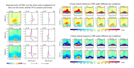
The greater quantities and larger sizes of liquid and solid cloud particles over the TP result in a much stronger SW cooling CRE and stronger LW heating CRE and net CRE at low altitudes and a much stronger SW heating CRE and stronger LW cooling CRE and net CRE at high altitudes there than over the Arctic. During boreal winter, the appearance of cooling LW and the net CRE at low altitudes over the Arctic is opposite to that over the TP, which may be associated with the distinct local atmospheric circulations over the two regions and the mechanism between them needs further research.

(3)

Further model calculations demonstrated the influence of the cloud microphysical distributions on the vertical structures of CREs. Ice cloud water primarily dominates the CRE vertical structures at high altitudes above 8 km, while cloud liquid water and mixed-phase cloud water (especially the liquid water in the mixed-phase clouds) primarily dominate the CRE vertical structures at low altitudes. The strong shallow heating layer above the cooling layer in the SW CRE and the strong shallow cooling layer above the heating layer in the LW CRE are primarily caused by cloud liquid water and mixed-phase water (especially the liquid water in the mixed-phase clouds). Compared with the Arctic, the cloud microphysics over the TP lead to very uneven vertical distributions of net CREs with a much stronger heating layer above the ground surface and almost comparable cooling layer above the heating layer caused by cloud water in the same phase.

The observational and modeling comparisons of the cloud microphysics and CREs over the two northern “poles” help us better understand cloud microphysics and its contributions to the vertical atmospheric structures of CREs. However, the vertical atmospheric CREs related to different cloud phases and the various microphysics in dynamical circulations and their underlying mechanisms require further research, which is essential to understand the roles played by the two northern “poles” in the local and global climate. Limited by the transit time of CloudSat/CALIPSO satellite, this study mainly reveals the characteristics on climatological scale, rigorous study of diurnal variation requires a combination of geostationary satellite and ground data synchronization. In the calculation of CRE through RRTM, the surface emissivity was set as the same no matter whether the surface ground was covered by ice or not which may cause a potential caveat [67,68], especially as the cloudy profiles increase atmospheric shortwave radiation [69]. The daily mean value of the solar zenith angle as input for the RRTM may be another caveat to the SW CRE calculated during warm seasons over the TP.

References

1. Harrison, E.F.; Minnis, P.; Barkstrom, B.R.; Ramanathan, V.; Cess, R.D.; Gibson, G.G. Seasonal variation of cloud radiative forcingderived from the Earth Radiation Budget Experiment. J. Geophys. Res. 1990, 95, 18687–18703. [Google Scholar] [CrossRef]
2. Stephens, G.L. Cloud feedbacks in the climate system: A critical review. J. Climate 2005, 18, 237–273. [Google Scholar] [CrossRef] [Green Version]
3. Koren, I.; Martins, J.V.; Remer, L.A.; Afargan, H. Smoke invigoration versus inhibition of clouds over the Amazon. Science 2008, 321, 946–949. [Google Scholar] [CrossRef] [Green Version]
4. Rosenfeld, D.; Lohmann, U.; Raga, G.B.; O’Dowd, C.; Kulmala, M.; Fuzzi, S.; Reissell, A.; Andreae, M.O. Flood or drought: How do aerosols affect precipitation? Science 2008, 321, 1309–1313. [Google Scholar] [CrossRef] [Green Version]
5. Andrews, T.; Forster, P.M.; Boucher, O.; Bellouin, N.; Jones, A. Forcing, feedbacks and climate sensitivity in CMIP5 coupled atmosphere–ocean climate models. Geophys. Res. Lett. 2012, 39, L09712. [Google Scholar] [CrossRef] [Green Version]
6. Jiang, J.H.; Su, H.; Zhai, C.; Perun, V.S.; Del Genio, A.; Nazarenko, L.S.; Donner, L.J.; Horowitz, L.; Seman, C.; Cole, J.; et al. Evaluation of cloud and water vapor simulations in CMIP5 climate models using NASA “A-Train” satellite observations. J. Geophys. Res. 2012, 117, D14105. [Google Scholar] [CrossRef] [Green Version]
7. Su, H.; Jiang, J.H.; Zhai, C.; Shen, T.J.; Neelin, J.D.; Stephens, G.L.; Yung, Y.L. Weakening and strengthening structures in the Hadley Circulation change under global warming and implications for cloud response and climate sensitivity. J. Geophys. Res. Atmos. 2014, 119, 5787–5805. [Google Scholar] [CrossRef] [Green Version]
8. Collins, M.; Knutti, R.; Arblaster, J.; Dufresne, J.-L.; Fichefet, T.; Friedlingstein, P.; Gao, X.; Gutowski, W.J.; Johns, T.; Krinner, G.; et al. Long-term climate change: Projections, commitments and irreversibility. In Climate Change 2013: The Physical Science Basis. Contribution of Working Group I to the Fifth Assessment Report of the Intergovernmental Panel on Climate Change; Cambridge University Press: Cambridge, UK; New York, NY, USA, 2013; pp. 1029–1136. [Google Scholar] [CrossRef]
9. Rangwala, I.; Sinsky, E.; Miller, J.R. Amplified warming projections for high altitude regions of the Northern Hemisphere mid-latitudes from CMIP5 models. Environ. Res. Lett. 2013, 8, 024040. [Google Scholar] [CrossRef]
10. Wu, G.; Zhang, Y. Tibetan Plateau forcing and the timing of the monsoon onset over South Asia and the South China Sea. Mon. Weather Rev. 1998, 126, 913–927. [Google Scholar] [CrossRef]
11. Duan, A.M.; Wu, G.X. Role of the Tibetan Plateau thermal forcing in the summer climate patterns over subtropical Asia. Clim. Dyn. 2005, 24, 793–807. [Google Scholar] [CrossRef]
12. Liu, Y.; Bao, Q.; Duan, A.; Qian, Z.; Wu, G. Recent progress in the impact of the Tibetan Plateau on climate in China. Adv. Atmos. Sci. 2007, 24, 1060–1076. [Google Scholar] [CrossRef]
13. Liu, Y.; Lu, M.; Yang, H.; Duan, A.; He, B.; Yang, S.; Wu, G. Land–atmosphere–ocean coupling associated with the Tibetan Plateau and its climate impacts. Natl. Sci. Rev. 2020, 7, 534–552. [Google Scholar] [CrossRef] [Green Version]
14. Fujinami, H.; Yasunari, T. The seasonal and intraseasonal variability of diurnal cloud activity over the Tibetan Plateau. J. Meteor. Soc. Jpn. 2001, 79, 1207–1227. [Google Scholar] [CrossRef] [Green Version]
15. Li, Y.; Liu, X.; Chen, B. Cloud type climatology over the Tibetan Plateau: A comparison of ISCCP and MODIS/TERRA measurements with surface observations. Geophys. Res. Lett. 2006, 33, L17716. [Google Scholar] [CrossRef]
16. Luo, Y.; Zhang, R.; Qian, W.; Luo, Z.; Hu, X. Inter-comparison of deep convection over the Tibetan Plateau–Asian monsoon region and subtropical north America in boreal summer using CloudSat/CALIPSO data. J. Clim. 2011, 24, 2164–2177. [Google Scholar] [CrossRef] [Green Version]
17. Rüthrich, F.; Thies, B.; Reudenbach, C.; Bendix, J. Cloud detection and analysis on the Tibetan Plateau using Meteosat and CloudSat. J. Geophys. Res. Atmos. 2013, 118, 10082–10099. [Google Scholar] [CrossRef]
18. Hong, Y.; Liu, G. The characteristics of ice cloud properties derived from CloudSat and CALIPSO measurements. J. Clim. 2015, 28, 3880–3901. [Google Scholar] [CrossRef]
19. Yan, Y.; Liu, Y.; Lu, J. Cloud vertical structure, precipitation, and cloud radiative effects over Tibetan Plateau and its neighboring regions. J. Geophys. Res. Atmos. 2016, 121. [Google Scholar] [CrossRef] [Green Version]
20. Yan, Y.-F.; Wang, X.-C.; Liu, Y.-M. Cloud vertical structures associated with precipitation magnitudes over the Tibetan Plateau and its neighboring regions. Atmos. Ocean. Sci. Lett. 2018, 11, 44–53. [Google Scholar] [CrossRef] [Green Version]
21. Yan, Y.; Liu, Y. Vertical structures of convective and stratiform clouds in boreal summer over the Tibetan Plateau and its neighboring regions. Adv. Atmos. Sci. 2019, 36, 1089–1102. [Google Scholar] [CrossRef]
22. Miao, H.; Wang, X.; Liu, Y.; Wu, G. An evaluation of cloud vertical structure in three reanalyses against CloudSat/cloud-aerosol lidar and infrared pathfinder satellite observations. Atmos. Sci. Lett. 2019, 20, e906. [Google Scholar] [CrossRef] [Green Version]
23. Lingen, B.; Longhua, L.; Changgui, L.; Yanjie, C.; Zhiqiu, G.; Huizhi, L.; Jiayi, C. The characteristics of radiation balance components of the Tibetan Plateau in the summer of 1998. Chin. J. Atmos. Sci. 2001, 25, 577–588. [Google Scholar]
24. CiRen, N.M.; DanZeng, L.B.; Xuan, Y.J.; Chen, T.L. Characteristic of seasonal variation of surface radiation balance at Yangbajin in Qinghai-Xizang plateau. Plateau Meteor. 2013, 32, 1253–1260. [Google Scholar] [CrossRef]
25. Su, W.; Mao, J.; Ji, F.; Qin, Y. Outgoing longwave radiation and cloud radiative forcing of the Tibetan plateau. J. Geophys. Res. Atmos. 2000, 105, 14863–14872. [Google Scholar] [CrossRef]
26. Naud, C.M.; Rangwala, I.; Xu, M.; Miller, J.R. A satellite view of the radiative impact of clouds on surface downward fluxes in the Tibetan plateau. J. Appl. Meteorol. Clim. 2012, 54, 479–493. [Google Scholar] [CrossRef]
27. Lu, J.; Cai, M. Seasonality of polar surface warming amplification in climate simulations. Geophys. Res. Lett. 2009, 36, L16704. [Google Scholar] [CrossRef]
28. Intrieri, J.; Fairall, C.; Shupe, M.D.; Persson, P.O.G.; Andreas, E.L.; Guest, P.S.; Moritz, R.E. An annual cycle of Arctic surface cloud forcing at SHEBA. J. Geophys. Res. Ocean. 2002, 107, 8039. [Google Scholar] [CrossRef]
29. Tjernström, M.; Sedlar, J.; Shupe, M.D. How well do regional climate models reproduce radiation and clouds in the Arctic? An evaluation of ARCMIP simulations. J. Appl. Meteorol. Clim. 2008, 47, 2405–2422. [Google Scholar] [CrossRef]
30. Kay, J.E.; Gettelman, A. Cloud influence on and response to seasonal Arctic Sea ice loss. J. Geophys. Res. Atmos. 2009, 114, D18204. [Google Scholar] [CrossRef]
31. Schweiger, A.J.; Lindsay, R.W.; Vavrus, S.; Francis, J.A. Relationships between Arctic Sea ice and clouds during autumn. J. Clim. 2008, 21, 4799–4810. [Google Scholar] [CrossRef]
32. Johansson, E.; Devasthale, A.; Tjernström, M.; Ekman, A.M.L.; L’Ecuyer, T. Response of the lower troposphere to moisture intrusions into the Arctic. Geophys. Res. Lett. 2017, 44, 2527–2536. [Google Scholar] [CrossRef]
33. Kay, J.E.; L’Ecuyer, T.; Gettelman, A.; Stephens, G.; O’Dell, C. The contribution of cloud and radiation anomalies to the 2007 Arctic Sea ice extent minimum. Geophys. Res. Lett. 2008, 35, L08503. [Google Scholar] [CrossRef] [Green Version]
34. Vavrus, S.; Holland, M.M.; Bailey, D.A. Changes in Arctic clouds during intervals of rapid sea ice loss. Clim. Dyn. 2011, 36, 1475–1489. [Google Scholar] [CrossRef] [Green Version]
35. Abe, M.; Nozawa, T.; Ogura, T.; Takata, K. Effect of retreating sea ice on Arctic cloud cover in simulated recent global warming. Atmos. Chem. Phys. 2016, 16, 14343–14356. [Google Scholar] [CrossRef] [Green Version]
36. Shupe, M.D.; Intrieri, J. Cloud radiative forcing of the Arctic surface: The influence of cloud properties, surface albedo, and solar zenith angle. J. Clim. 2004, 17, 616–628. [Google Scholar] [CrossRef]
37. Francis, J.A.; Hunter, E. New insight into the disappearing arctic sea ice. EOS Trans. Am. Geophys. Union 2006, 87, 509–524. [Google Scholar] [CrossRef]
38. Wyser, K.; Jones, C.G.; Du, P.; Girard, E.; Willén, U.; Cassano, J.; Christensen, J.H.; Curry, J.A.; Dethloff, K.; Haugen, J.-E.; et al. An evaluation of Arctic cloud and radiation processes during the SHEBA year: Simulation results from eight Arctic regional climate models. Clim. Dyn. 2008, 30, 203–223. [Google Scholar] [CrossRef] [Green Version]
39. Klein, S.A.; McCoy, R.B.; Morrison, H.; Ackerman, A.; Avramov, A.; de Boer, G.; Chen, M.; Cole, J.N.S.; Del Genio, A.D.; Falk, M.; et al. Intercomparison of model simulations of mixed-phase clouds observed during the ARM Mixed-Phase Arctic Cloud Experiment. I: Single-layer cloud. Quart. J. Roy. Meteor. Soc. 2009, 135, 979–1002. [Google Scholar] [CrossRef]
40. Morrison, H.; McCoy, R.B.; Klein, S.; Xie, S.; Luo, Y.; Avramov, A.; Chen, M.; Cole, J.N.S.; Falk, M.; Foster, M.J.; et al. Intercomparison of model simulations of mixed-phase clouds observed during the ARM Mixed-Phase Arctic Cloud Experiment. II: Multilayer cloud. Quart. J. Roy. Meteor. Soc. 2009, 135, 1003–1019. [Google Scholar] [CrossRef]
41. De Boer, G.; Tripoli, G.J.; Eloranta, E.W. Preliminary comparison of CloudSAT-derived microphysical quantities with ground-based measurements for mixed-phase cloud research in the Arctic. J. Geophys. Res. 2008, 113, D00A06. [Google Scholar] [CrossRef] [Green Version]
42. Gayet, J.-F.; Mioche, G.; Dörnbrack, A.; Ehrlich, A.; Lampert, A.; Wendisch, M. Microphysical and optical properties of arctic mixed-phase clouds—the 9 April 2007 case study. Atmos. Chem. Phys. 2009, 9, 6581–6595. [Google Scholar] [CrossRef] [Green Version]
43. Solomon, A.; Morrison, H.; Persson, O.; Shupe, M.D.; Bao, J.-W. Investigation of microphysical parameterizations of snow and ice in arctic clouds during m-pace through model-observation comparisons. Mon. Weather Rev. 2009, 137, 3110–3128. [Google Scholar] [CrossRef] [Green Version]
44. Walsh, J.E.; Chapman, W.L.; Portis, D.H. Arctic cloud fraction and radiative fluxes in atmospheric reanalyses. J. Clim. 2009, 22, 2316–2334. [Google Scholar] [CrossRef]
45. Dong, X.; Xi, B.; Crosby, K.; Long, C.N.; Stone, R.S.; Shupe, M.D. A 10 year climatology of Arctic cloud fraction and radiative forcing at Barrow, Alaska. J. Geophys. Res. 2010, 115, D17212. [Google Scholar] [CrossRef]
46. Sedlar, J.; Tjernström, M.; Mauritsen, T.; Shupe, M.D.; Brooks, I.; Persson, P.O.G.; Birch, C.E.; Leck, C.; Sirevaag, A.; Nicolaus, M. A transitioning Arctic surface energy budget: The impacts of solar zenith angle, surface albedo and cloud radiative forcing. Clim. Dyn. 2010, 37, 1643–1660. [Google Scholar] [CrossRef] [Green Version]
47. Hoeve, J.E.T.; Remer, L.A.; Jacobson, M.Z. Microphysical and radiative effects of aerosols on warm clouds during the amazon biomass burning season as observed by Modis: Impacts of water vapor and land cover. Atmos. Chem. Phys. 2011, 11, 3021–3036. [Google Scholar] [CrossRef] [Green Version]
48. Shupe, M.D.; Turner, D.D.; Zwink, A.; Thieman, M.M.; Mlawer, E.J.; Shippert, T. Deriving arctic cloud microphysics at barrow, alaska: Algorithms, results, and radiative closure. J. Appl. Meteorol. Clim. 2015, 54, 1675–1689. [Google Scholar] [CrossRef]
49. Yan, Y.; Liu, X.; Liu, Y.; Lu, J. Comparison of mixed-phase clouds over the Arctic and the Tibetan Plateau: Seasonality and vertical structure of cloud radiative effects. Clim. Dyn. 2020, 54, 4811–4822. [Google Scholar] [CrossRef]
50. Stephens, G.L.; Vane, D.G.; Boain, R.J.; Mace, G.G.; Sassen, K.; Wang, Z.; Illingworth, A.J.; O’Connor, E.J.; Rossow, W.B.; Durden, S.L.; et al. The cloudsat mission and the A-train. Bull. Am. Meteor. Soc. 2002, 83, 1771–1790. [Google Scholar] [CrossRef] [Green Version]
51. Winker, D.M.; Hunt, W.H.; McGill, M.J. Initial performance assessment of CALIOP. Geophys. Res. Lett. 2007, 34, L19803. [Google Scholar] [CrossRef] [Green Version]
52. Austin, R. Level 2B Radar-Only Cloud Water Content (2B-CWC-RO) Process Description Document. CloudSat Project Report. 2007, p. 24. Available online: http://www.cloudsat.cira.colostate.edu/data-products/level-2b/2b-cwc-ro?term=28 (accessed on 29 April 2020).
53. Austin, R.T.; Heymsfield, A.J.; Stephens, G.L. Retrieval of ice cloud microphysical parameters using the CloudSat millimeter-wave radar and temperature. J. Geophys. Res. 2009, 114, D00A23. [Google Scholar] [CrossRef] [Green Version]
54. L’Ecuyer, T.S.; Wood, N.B.; Haladay, T.; Stephens, G.L.; Stackhouse, P.W. Impact of clouds on atmospheric heating based on the R04 CloudSat fluxes and heating rates data set. J. Geophys. Res. 2008, 113, D00A15. [Google Scholar] [CrossRef] [Green Version]
55. A NASA Earth System Science Pathfinder Mission. Level 2B Fluxes and Heating Rates and 2B Fluxes and Heating Rates w/Lidar Process Description and Interface Control Document, Version 1.0. CloudSat Project Report; 2011; p. 28. Available online: http://www.cloudsat.cira.colostate.edu/data-products/level-2b/2b-flxhr-lidar?term=38 (accessed on 29 April 2020).
56. Henderson, D.S.; L’Ecuyer, T.; Stephens, G.L.; Partain, P.; Sekiguchi, M. A multisensor perspective on the radiative impacts of clouds and aerosols. J. Appl. Meteorol. Clim. 2013, 52, 853–871. [Google Scholar] [CrossRef]
57. Heymsfield, A.J.; Protat, A.; Bouniol, D.; Austin, R.T.; Hogan, R.J.; Delanoë, J.; Okamoto, H.; Sato, K.; Van Zadelhoff, G.-J.; Donovan, D.P.; et al. Testing IWC retrieval methods using radar and ancillary measurements with in situ data. J. Appl. Meteorol. Clim. 2008, 47, 135–163. [Google Scholar] [CrossRef] [Green Version]
58. Mlawer, E.J.; Taubman, S.J.; Brown, P.D.; Iacono, M.J.; Clough, S.A. RRTM, a validated correlated-k model for the longwave. J. Geophys. Res. 1997, 102, 16663–16682. [Google Scholar] [CrossRef] [Green Version]
59. Wang, X.; Miao, H.; Liu, Y.; Bao, Q. Dependence of cloud radiation on cloud overlap, horizontal inhomogeneity, and vertical alignment in stratiform and convective regions. Atmos. Res. 2021, 249, 105358. [Google Scholar] [CrossRef]
60. Clough, S.; Shephard, M.; Mlawer, E.; Delamere, J.; Iacono, M.; Cady-Pereira, K.; Boukabara, S.; Brown, P. Atmospheric radiative transfer modeling: A summary of the AER codes. J. Quant. Spectrosc. Radiat. Transf. 2005, 91, 233–244. [Google Scholar] [CrossRef]
61. Morcrette, J.-J.; Barker, H.W.; Cole, J.N.S.; Iacono, M.; Pincus, R. Impact of a new radiation package, McRad, in the ECMWF integrated forecasting system. Mon. Weather Rev. 2008, 136, 4773–4798. [Google Scholar] [CrossRef]
62. Hu, Y.X.; Stamnes, K. An accurate parameterization of the radiative properties of water clouds suitable for use in climate models. J. Clim. 1993, 6, 728–742. [Google Scholar] [CrossRef] [Green Version]
63. Fu, Q. An accurate parameterization of the solar radiative properties of cirrus clouds for climate models. J. Clim. 1996, 9, 2058–2082. [Google Scholar] [CrossRef] [Green Version]
64. Coakley, J.A., Jr.; Cess, R.D.; Yurevich, F.B. The effect of tropospheric aerosols on the Earth’s radiation budget: A parameterization for climate models. J. Atmos. Sci. 1983, 40, 116–138. [Google Scholar] [CrossRef] [Green Version]
65. Ramanathan, V.; Cess, R.D.; Harrison, E.F.; Minnis, P.; Barkstrom, B.R.; Ahmad, E.; Hartmann, D. Cloud-radiative forcing and climate: Results from the Earth radiation budget experiment. Science 1989, 243, 57–63. [Google Scholar] [CrossRef] [PubMed] [Green Version]
66. Matus, A.V.; L’Ecuyer, T.S. The role of cloud phase in Earth’s radiation budget. J. Geophys. Res. Atmos. 2017, 122, 2559–2578. [Google Scholar] [CrossRef]
67. Berry, E.; Mace, G.G. Cloudproperties and radiative effects of the Asian summer monsoon derived from A-Train data. J. Geophys. Res. Atmos. 2014, 119, 9492–9508. [Google Scholar] [CrossRef]
68. Campbell, J.R.; Dolinar, E.K.; Lolli, S.; Fochesatto, G.J.; Gu, Y.; Lewis, J.R.; Marquis, J.W.; McHardy, T.M.; Ryglicki, D.R.; Welton, E.J. Cirrus cloud Top-of-the-Atmosphere net daytime forcing in the Alaskan subarctic from ground-based MPLNET monitoring. J. Appl. Meteorol. Clim. 2021, 60, 51–63. [Google Scholar] [CrossRef]
69. Zelinka, M.D.; Klein, S.; Hartmann, D.L. Computing and partitioning cloud feedbacks using cloud property histograms. Part I: Cloud radiative kernels. J. Clim. 2012, 25, 3715–3735. [Google Scholar] [CrossRef] [Green Version]
Figure 1. Seasonal cycle of the vertical distribution of the cloud ice (upper panels),(a,b) and liquid (lower panels),(c,d) number concentrations over the Tibetan Plateau (TP; left panels),(a,c) and the Arctic (right panels),(b,d). The upper and lower black lines in each plot represent the climatic locations of −20 and 0 °C that are calculated from the ECMWF–aux (version r04) product.
Remotesensing 13 02651 g001
Figure 2. Seasonal cycle of the vertical distribution of the cloud ice (upper panels),(a,b) and liquid (lower panels),(c,d) particle effective radius over the TP (left panels),(a,c) and the Arctic (right panels),(b,d). The upper and lower black lines in each plot represent the climatic locations of −20 and 0 °C that are calculated from the ECMWF–aux (version r04) product.
Remotesensing 13 02651 g002
Figure 3. Seasonal cycle of the vertical profile of the cloud radiation effects (CRE) per unit mass over (a,d,g) the Arctic and a comparison of the vertical profile of CRE per unit mass over the Arctic (blue) and the TP (red) in (b,e,h) boreal summer and (c,f,i) boreal winter for the (ac) shortwave (SW), (df) longwave (LW), and (gi) net (SW+LW) CRE. The grey lines in the center and right panels represent 0 K day−1.
Remotesensing 13 02651 g003
Figure 4. Rapid Radiative Transfer Model (RRTM) calculation results for the seasonal cycle of the cloud vertical SW CRE under different sky conditions per unit mass over (af) the TP and (gl) the Arctic. Panels (a) and (g) show the cloud ice or liquid water contained in the atmospheric profiles; panels (b) and (h) show only the cloud ice water; panels (c) and (i) show only cloud water; panels (d) and (j) show only the mixed-phase cloud water layer; panels (e) and (k) show only the ice water portion in the mixed-phase clouds; panels (f) and (l) show only the liquid water portion in the mixed-phase clouds. Positive and negative values represent the heating and cooling rates, respectively. Unit: K day−1.
Remotesensing 13 02651 g004
Figure 5. As in Figure 4, but for the LW CRE.
Remotesensing 13 02651 g005
Figure 6. RRTM calculation results for the seasonal cycle of the cloud net (SW+LW) CRE under different sky conditions per unit mass over (ad) the TP and (eh) the Arctic. Panels (a) and (e) show the cloud ice or liquid water contained in the atmospheric profiles; panels (b) and (f) show only the cloud ice water; panels (c) and (g) show only the cloud liquid water; panels (d) and (h) show only the mixed-phase cloud water layer. Positive and negative values represent the heating and cooling rates, respectively. Unit: K day−1.
Remotesensing 13 02651 g006
Publisher’s Note: MDPI stays neutral with regard to jurisdictional claims in published maps and institutional affiliations.