Review

Performance Comparison of Filtering Algorithms for High-Density Airborne LiDAR Point Clouds over Complex LandScapes

1
Key Laboratory of Geomatics and Digital Technology of Shandong Province, Shandong University of Science and Technology, Qingdao 266590, China
2
College of Geodesy and Geomatics, Shandong University of Science and Technology, Qingdao 266590, China
*
Author to whom correspondence should be addressed.
Remote Sens. 2021, 13(14), 2663; https://doi.org/10.3390/rs13142663
Submission received: 7 June 2021 / Revised: 5 July 2021 / Accepted: 5 July 2021 / Published: 7 July 2021

Abstract

:
Airborne light detection and ranging (LiDAR) technology has become the mainstream data source in geosciences and environmental sciences. Point cloud filtering is a prerequisite for almost all LiDAR-based applications. However, it is challenging to select a suitable filtering algorithm for handling high-density point clouds over complex landscapes. Therefore, to determine an appropriate filter on a specific environment, this paper comparatively assessed the performance of five representative filtering algorithms on six study sites with different terrain characteristics, where three plots are located in urban areas and three in forest areas. The representative filtering methods include simple morphological filter (SMRF), multiresolution hierarchical filter (MHF), slope-based filter (SBF), progressive TIN densification (PTD) and segmentation-based filter (SegBF). Results demonstrate that SMRF performs the best in urban areas, and compared to MHF, SBF, PTD and SegBF, the total error of SMRF is reduced by 1.38%, 48.21%, 48.25% and 31.03%, respectively. MHF outperforms the others in forest areas, and compared to SMRF, SBF, PTD and SegBF, the total error of MHF is reduced by 1.98%, 35.87%, 45.11% and 9.42%, respectively. Moreover, both SMRF and MHF keep a good balance between type I and II errors, which makes the produced DEMs much similar to the references. Overall, SMRF and MHF are recommended for urban and forest areas, respectively, and MHF averagely performs slightly better than SMRF on all areas with respect to kappa coefficient.

1. Introduction

Airborne light detection and ranging (LiDAR) technology has been widely accepted as a powerful tool for generating high-quality digital elevation models (DEMs) [1,2]. Compared to the classical surveying and mapping methods, LiDAR shows many promising merits, such as the high efficiency for collecting high-density and large-scale point clouds, which is conducive to the detailed representation of topography [3,4], and forest canopy penetration ability, which is valuable for forest inventory and management [5,6]. Generally, the raw LiDAR point clouds include not only the bare earth (BE) points, but also the object (OBJ) points, which make point cloud filtering indispensable for almost all LiDAR-based applications, such as landslide detection [7], erosion and deposition quantification [8], channel-bed morphology recognition [9] and individual tree position extraction [10].
During the past two decades, plenty of filtering algorithms have been presented. However, each method has its strengths and weaknesses for handling different landscapes, and the performances of these filtering algorithms vary from one scene to another. Thus, performance comparison between the filtering algorithms is highly beneficial for the choice of an appropriate filter, especially for inexperienced users.
To fill this gap, Sithole and Vosselman [11] compared the performances of eight filtering algorithms on the International Society for Photogrammetry and Remote Sensing (ISPRS) benchmark dataset, and found that adaptive triangulated irregular network (ATIN) (also termed as progressive TIN densification, PTD) outperformed the others, since it used more context. Zhang and Whitman [12] compared three filtering algorithms including the elevation threshold with expanding window (ETEW), maximum local slope (MLS), and progressive morphological filter (PM) on the datasets in urban, mountainous and coastal areas. Results indicated that the PM method yielded the highest accuracy in urban and coastal areas, while MLS performs well for the removal of low vegetation in high-relief areas. Meng et al. [13] classified the existing filtering algorithms into six categories based on their characteristics, and further demonstrated the high accuracy of ATIN on the ISPRS dataset. Tinkham et al. [14] assessed two open source point classification algorithms including Multiscale Curvature Classification (MCC) [15] and Boise Center Aerospace Laboratory LiDAR algorithm (BCAL) in a semi-arid watershed with mixed vegetation types. Results showed that BCAL produced more accurate surfaces in very dense and continuous vegetation, while in areas where steep or sudden changes in slope, MCC outperformed BCAL. Julge et al. [16] evaluated the performance of six common filtering algorithms embedded in three freeware programs on four areas with different landscapes. The filters include ATIN, ETEW, MLS, PM, MCC and weighted linear prediction (WLP). They concluded that MCC produced the smallest DEM root mean square errors (RMSEs) in the test areas. Korzeniowska et al. [17] proposed an evaluation of four filtering algorithms including PM, PTD, WLP and segmentation-based filter on eight test sites with different landscapes. The results showed that no single method was consistently more accurate than the others for all types of terrain. Montealegre et al. [18] evaluated the performance of seven filtering algorithms including ATIN, WLP, MCC, BCAL, ETEW, PM and MLS in two forested sites. Results demonstrated that MCC achieved the highest accuracy. Zhao et al. [19] compared the results of MCC, WLP, MF, ATIN, and the slope-based filter (SBF) in vegetated mountain areas and indicated that the performance of each method varied under different landscapes. Specifically, SBF and MCC produced the highest accuracy in flat areas and steep and dense forests, respectively, while WLP and MCC showed good performance in steep and sparely vegetated areas. Although many comparison studies have been conducted between the filtering algorithms, their performance were mainly assessed based on low-density point clouds (<10 points/m2).
With the rapid development of hardware equipment, the collection of high-density point clouds becomes more and more convenient. However, filtering high-density point clouds is more challenging than those of the low-density [20], which is mainly due to the facts that (i) high-density point clouds result in more abnormal points; (ii) high-density data make parameter setting more difficult, and the improper parameter setting could lead to poor results; and (iii) high-density data include more information, and the rich information cannot easily be handled. Montealegre et al. [18] showed that the Type II errors increase as the point density increases. Serifoglu Yilmaz and Gungor [20] indicated that with the increase of point density, the performance of the filtering algorithm decreases.
Nevertheless, few studies have been conducted to compare the performance of filtering algorithms on high-density point clouds. Serifoglu Yilmaz et al. [21] investigated the results of PM, ETEW, ATIN, MCC, BCAL, gLiDAR and cloth simulation filter (CSF) on unmanned aerial vehicles (UAV)-based high-density point clouds in two study sites with simple landscapes, and found that CSF produced the lowest total errors. Zeybek and Şanlıoğlu [22] obtained the same conclusion to that of Serifoglu Yilmaz et al. [21] in four study sites with simple landscapes. Serifoglu Yilmaz and Gungor [20] compared the performance of PM1D/2D, MLS, ETEW and ATIN on UAV-based high-density point clouds in a small study area, and regarded ATIN as the best method. Klápště et al. [23] compared six filtering algorithms in a study site with sparsely distributed vegetation and found that no universal method can outperform the others. From above discussion, it can be seen that the landscapes adopted in their research are simple and single, which cannot comprehensively assess the performance of the filtering algorithms. Moreover, the aforementioned studies mainly filtered the UAV-based photogrammetry point clouds, and their conclusions might not be suitable for LiDAR-based data due to their different data collection manners [24]. Thus, further investigation should be performed on high-density LiDAR point clouds over complex landscapes.
Based on the aforementioned discussion, the objective of this paper is to comparatively assess the performance of five representative filtering algorithms of different types on airborne LiDAR-based high-density point clouds over complex landscapes, thereby specifying an optimum filter for one specific scene. Compared to previous studies, the main contributions of this paper are as follows: (i) the types of filtering algorithms in the comparison are manifold. Specifically, almost all types of filters are used, including nonlinear (linear) interpolation-based, slope-based, morphology-based and segmentation-based filters. Thus, the performance of different types could be compared. (ii) The landscapes of the six plots located in forest and urban areas are complex. Therefore, the merits and shortcomings of each filter on different landscapes could be obtained. (iii) The airborne LiDAR point clouds on all the plots are high-density. This caters to the development of LiDAR systems, since more advanced LiDAR systems are being developed in recent years and the data density of the collected point clouds becomes increasingly higher. In a word, we employed six groups of high-density LiDAR point clouds over different complex landscapes to comprehensively assess the performance of five types of filters, which would contribute to the selection of a suitable filter over a specified landscape.
The remainder of this paper is organized as follows. The classical filtering algorithms are reviewed in Section 2. Section 3 introduces the experiments. Results are analyzed in Section 4. Discussion and conclusion are given in Section 5 and Section 6, respectively.

2. Related Works

According to their working principles, the existing filtering methods can be roughly classified into five categories: slope-based, morphology-based, interpolation-based, segmentation-based and machine learning-based algorithms.

2.1. Slope-Based Filters

The slope-based filters are based on the assumption that the large slope between two nearby points is mainly caused by an OBJ point, i.e., the higher one [25]. In other words, one point is flagged as the BE if the maximum slope between this point and its neighbors does not exceed the predefined tolerance. To improve the performance on steep slopes, some adaptive slope-based filters were developed [26,27], where the slope threshold adaptively changes with respect to terrain slope (Figure 1). Moreover, some scholars [28,29] enhanced the slope-based filters with the inclusion of elevation difference threshold. Generally, the slope-based filters have the advantages of simplicity and efficiency. However, they are highly sensitive to slope threshold, especially in areas with abrupt terrain [30].

2.2. Morphology-Based Filters

Morphology-based filters are mainly based on two fundamental operations, i.e., dilation and erosion. The combination of dilation and erosion produces opening and closing operations, which are employed to filter point clouds in the morphology-based filters (Figure 2). More specifically, the raw point clouds are first rasterized based on the lowest points within a given window size, and then processed with the opening operation. Finally, points with elevation differences before and after the operations greater than the tolerance are flagged as OBJ points [31]. However, the performance of the morphology-based filters is greatly influenced by the window size, which cannot keep a good tradeoff between the removal of large-size objects and the preservation of detailed ground points. Thus, progressive morphological filters were proposed [32,33], where the window size of the filter and elevation difference threshold are gradually increasing. Since the morphological filters operate on the rasterized point clouds, they have a low computational cost. However, the transformation from the raw point cloud into the rasterized image inevitably causes information loss, especially in steep slope areas.

2.3. Interpolation-Based Filters

Generally, the interpolation-based filters first select some initial ground seeds using a moving window with the size slightly larger than the maximum object, and then interpolate these ground seeds using an interpolation method. Finally, new ground points are detected when their vertical distances to the interpolated surface are less than the given elevation threshold. ATIN proposed by Axelsson [34] (Figure 3) is considered as a representative of interpolation-based filters. Due to its high filtering accuracy and integration into the commercial software named TerrainSolid, ATIN gains considerable attention [35]. Thus, many studies focused on its enhancement with respect to the selection of ground seeds, parameter setting, iterative judgment criterion and TIN construction [36,37,38,39,40]. Considering the inaccuracy of TIN for describing complex terrain surface, many advanced interpolation methods are recommended to replace TIN for reference ground surface construction, such as linear prediction [41], thin plate spline [15,42,43,44] and cubic spline interpolation [45]. Although the interpolation-based filters are praised for their filtering accuracy, they suffer from a large computational cost.

2.4. Segmentation-Based Filters

Segmentation-based filters first divide the point cloud into segments using some algorithms, such as region growing [37,46] and scanline segmentation [47], and then label each segment as BE or OBJ, where points in the same segments have the same labels (Figure 4). The advantages of the segmentation-based filters include the preservation of terrain break lines and the resistance of sample noise [24,48]. However, their performance significantly depends on the quality of segmentation, and the poor segmented results could offset the merits of the segmentation-based filters [49].

2.5. Machine learning-Based Filters

Recently, some machine learning-based filters have been proposed based on machine learning methods (Figure 5), such as artificial neural network [50], convolutional neural networks (CNN) [51,52,53,54] and AdaBoost [55,56]. Moreover, Yilmaz et al. [57] investigated the performance of some state-of-the-art machine learning algorithms including artificial neural network (ANN), support vector machines (SVM), and random forest (RF) for filtering UAS-based point clouds, and found that SVM-based filter outperformed the others. However, this kind of filter requires a sufficient number of training points to construct the model, and the production of training data with different types is rather challenging and subjective.
It is well known that machine learning-based filters are not easy-to-use since they require a large number of labeled points to train the model and the quality of the sample points seriously influences their performance. Moreover, if the labeled points were used to train the machine learning-based filter, its performance cannot be objectively compared with those of other filters, since the latter do not require training points. Thus, the machine learning-based filter was not adopted in our following experiments.

3. Experiments

To fully compare the performance of state-of-the-art filtering algorithms under different landscapes, six datasets with complex landscapes were employed in the experiments.

3.1. Filtering Algorithms

The filtering algorithms were selected based on the rules that they are classical, representative and easy-to-use. Thus, five filtering algorithms were adopted including multiresolution hierarchical filter (MHF), progressive TIN densification (PTD), region growing segmentation-based filter (SegBF), simple morphological filter (SMRF) and the maximum local slope-based filter (SBF). The detailed information of each algorithm is introduced in the following subsections.

3.1.1. Multiresolution Hierarchical Filter (MHF)

MHF belongs to the nonlinear interpolation-based filters, which was originally developed by Chen et al. [42]. During point cloud filtering, it first selects initial ground seeds using a moving window with the size slightly larger than the maximum OBJ. Then, the ground seeds are interpolated by thin plate spline (TPS) to produce a reference ground surface. Finally, for each candidate point, 9 height differences are computed by comparing its elevation with those of the grid cell where it is located and its 8 neighboring grid cells. Thus, if at least four height differences are less than the given threshold, the point is flagged as BE, and then added to the ground seeds. MHF includes three parameters: maximum window size, initial DEM resolution and initial elevation difference threshold.

3.1.2. Progressive TIN Densification (PTD)

PTD is a simple linear interpolation-based filter. The method was proposed by Axelsson [34]. It works as follows: the initial ground seeds are first selected with the same manner as MHF. Then, the TIN surface is constructed using the Delaunay triangulation algorithm on the ground seeds. For each candidate point, if its vertical distance to the corresponding triangle surface and the maximum of the three angles between the triangle surface and lines connecting the candidate and vertices of the triangle are less than the given thresholds, the point is flagged as BE. The above steps are repeated until no ground points are selected. PTD has four primary parameters: maximum window size, grid cell size, elevation difference threshold and angle threshold.

3.1.3. Region Growing Segmentation-Based Filter (SegBF)

The implementation of SegBF is based on the method of [58]. Specifically, the region growing algorithm is first used to group the point cloud into segments. Then, the ground segments are selected based on their properties using threshold values. SegBF includes three main parameters: search radius for plane fitting, maximum difference of normal vectors and maximum difference in elevation between neighboring points in the same segment.

3.1.4. Simple Morphological Filter (SMRF)

SMRF [33] belongs to the morphology-based filters. It adopts a linearly increasing window and simple slope thresholding, together with an image inpainting technique to filter point clouds. More specifically, the minimum surface is first produced with the image inpainting method. Then, the minimum surface is iteratively processed with the opening operation, and the OBJ points are removed based on the elevation differences before and after the process. Next, the DEM is generated based on the remaining BE points. Finally, the raw point clouds are classified as BE or OBJ based on their vertical differences to the generated DEM. SMRF has five parameters: the cell size of the minimum surface grid, a percent slope value, elevation difference threshold, slope threshold and maximum window size.

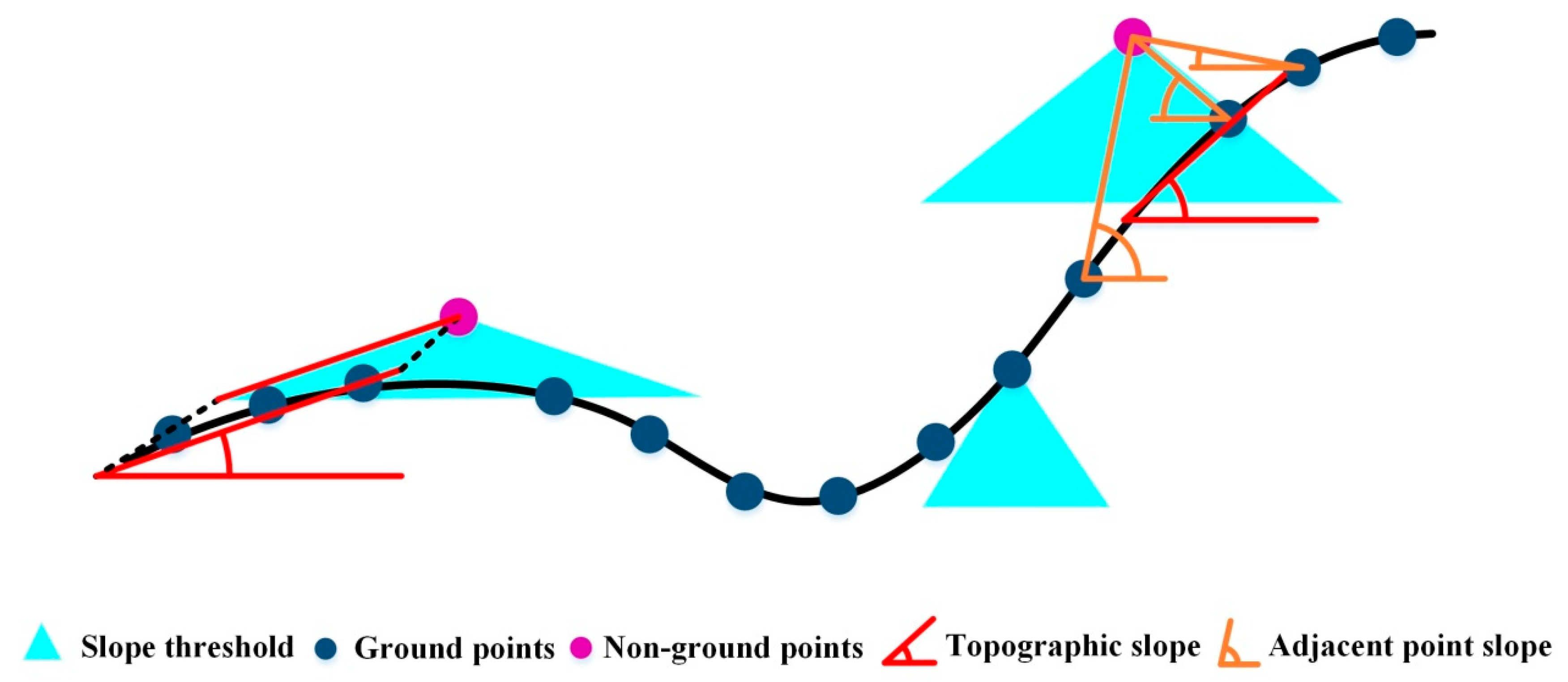
3.1.5. Slope-Based Filter (SBF)

The implementation of SBF is based on the method of [25]. It works as follows. Firstly, the raw point cloud is covered with grid cells. Then, the minimum point is selected for each grid cell. Finally, a point is labelled as BE if the maximum slope between this point and its neighbors within a predefined distance is less than a tolerance. SBF includes three parameters: grid cell resolution, slope threshold and search distance.

3.2. Datasets

Six datasets with different terrain characteristics were employed to assess the performance of the classical filtering algorithms, where three (plots 1–3) are located in urban sites and three (plots 4–6) in forest sites (Figure 6). The detailed information for data collection is shown in Table 1.
Table 2 shows the landscape characteristics of the six datasets including point density, mean terrain slope and OBJ cover rate. It can be seen that the six datasets have high data density (>10 points/m2), the mean slope ranges from 8.84° to 31.76°, and the OBJ coverage rate from 54.45% to 94.51%. All these information indicates the high complexity of the landscapes, which make them greatly challenging for the classical filtering algorithms. To produce reference samples for each dataset, the raw point cloud was first automatically filtered using the software Terrascan, and then the filtered data were manually edited to assure their accuracy. The number of BE points (#BE) and that of OBJ points (#OBJ) are shown in Figure 7. The reference DEMs for the six datasets interpolated on the filtered BE points are shown in Figure 8, which clearly illustrate the terrain characteristics.

3.3. Accuracy Measures

Four accuracy measures including type I, type II and total errors, and kappa coefficient [11,33,42] were adopted to quantitatively assess the performances of the filtering algorithms. Type I (T.I) error equals to the number of BE points misclassified as the OBJ points divided by the true number of BE points. Type II (T.II) error equals to the number of OBJ points misclassified as the BE points divided by the true number of OBJ points. Total error (T.E) equals to the sum of all misclassified points divided by the total number of points. Kappa coefficient (κ) measures the overall agreement between two judges, while considering the possibility of chance in the observed frequencies. The four measures are respectively formulated as
T.I = b a + b × 100 %
T.II = c c + d × 100 %
T.E = b + c e × 100 %
κ = p 0 p c 1 p c × 100 %
where a is the accurately classified BE points, b is the misclassified BE points, c is the misclassified OBJ points, d is the accurately classified OBJ points; e = a + b + c + d ; p 0 = ( a + d ) / e ; p c = ( ( a + b ) × ( a + c ) + ( c + d ) × ( b + d ) ) / e 2 .

4. Results

To give fair comparison between the filtering algorithms, their optimal parameters were empirically chosen in terms of the minimum total error on each plot.

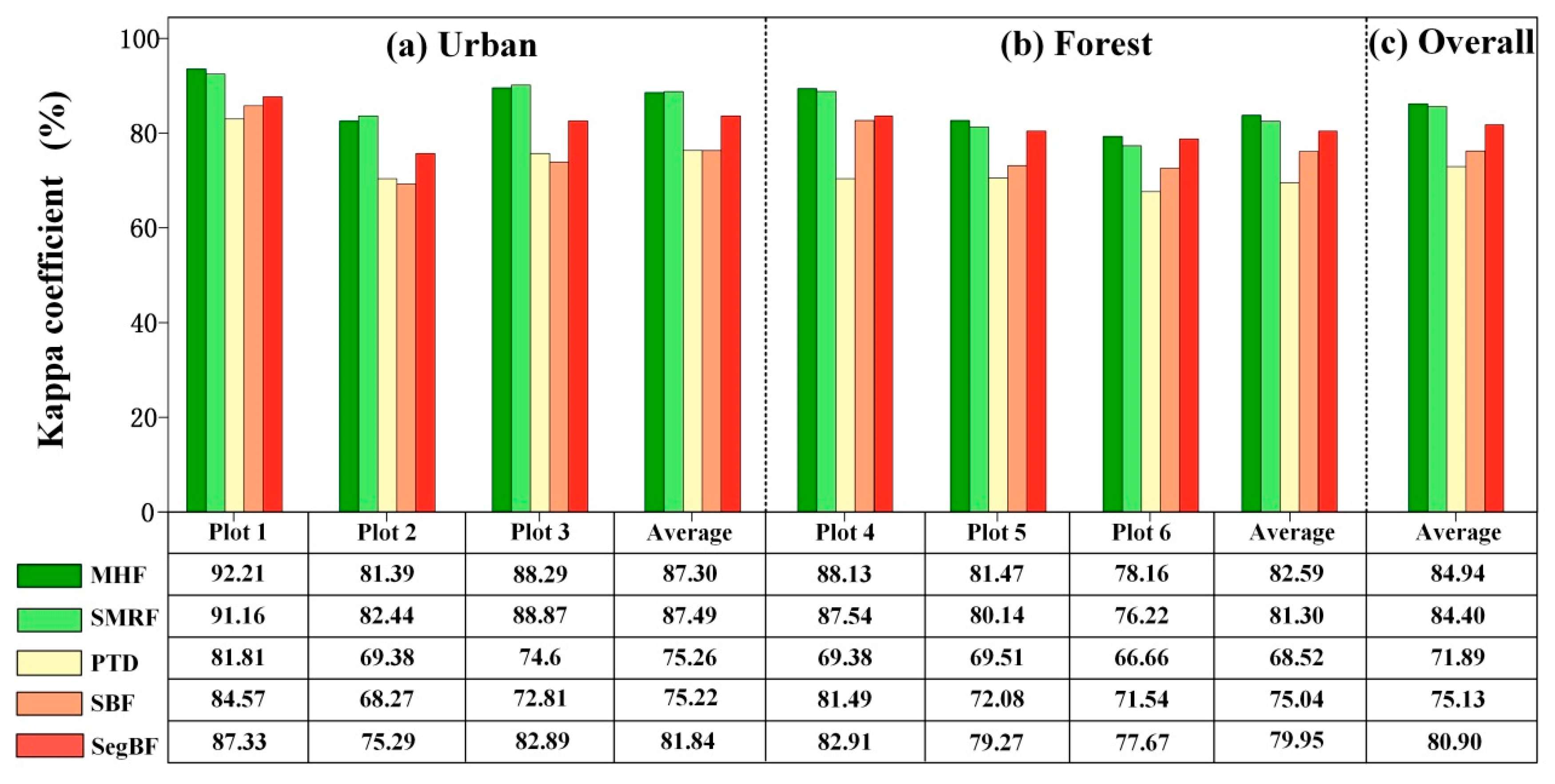
4.1. Kappa Coefficient

Figure 9 illustrates the kappa coefficients of all the filtering algorithms on the six plots. Results show that in urban areas, the kappa coefficient ranges from 68.27% on plot 2 to 92.21% on plot 1, while in forest areas, the kappa coefficient varies from 66.66% on plot 6 to 88.13% on plot 4. This indicates the higher accuracy in urban areas than in forest areas, which is mainly due to a sparse distribution of BE points in the latter (Figure 7). For the three urban areas, plot 1 with the flattest terrain (Figure 8a) has the best result, while plot 2 with the most complex terrain (Figure 8b) has the worst one. In the forest areas, plot 6 with the largest canopy cover (Table 2) produces the lowest accuracy, and plot 4 with the smallest canopy cover (Table 2) obtains the highest accuracy. In conclusion, both terrain complexity and canopy cover have a great effect on the performance of the filtering algorithms. This conclusion is consistent with those of previous studies. For example, Montealegre et al. [18] showed that most filtering algorithms produced larger errors with the increase of terrain complexity. Zhao et al. [19] indicated that filtering errors increase with the increase of canopy cover when the latter is greater than 80%.
Accuracy comparison between the filtering algorithms demonstrates that in urban areas, SMRF produces the best results on almost all plots except for plot 1, which is closely followed by MHF. SegBF is less accurate than MHF. The accuracy of SBF is approximate to that of PTD. On average, the five methods can be classified into three ranks based on their filtering accuracy. Specifically, SMRF and MHF with the kappa coefficients greater than 87% belong to the first rank, SegBF with the value greater than 81% is the second rank, while SBF and PTD with the values greater than 75% belong to the last rank. Note that the kappa coefficient difference between the maximum and minimum values is 12.27%, which demonstrates the significance for filter selection in the urban areas.
In the forest areas, MHF yields the best performance on all plots, while PTD produces the worst performance. On average, MHF with the kappa coefficient of 82.59% ranks the first, SMRF with the value of 81.30% ranks the second, SegBF with the value of 79.95% ranks the third, SBF with the value of 75.04% ranks the fourth, while PTD with the value of 68.52% ranks the last. This shows that kappa coefficient range between the best and worst methods reaches to 14.07%, indicating that method selection is also important in forest areas.
Overall, MHF (84.94%) has the highest accuracy, which is closely followed by SMRF (84.40%), whereas PTD (71.89%) produces the worst performance.

4.2. Type I, II and Total Errors

The type I, II and total errors of all the filtering algorithms are shown in Figure 10. In the urban areas, SMRF, MHF and SegBF have larger type II errors than type I errors, while SBF and PTD produce larger type I errors than type II errors. However, the type II errors of SMRF and MHF are much less than those of the other methods, which results in their smaller total errors. In comparison, PTD and SBF produce the largest total errors, with the mean values of 11.17% and 11.16%, respectively. They are about two times as large as those of SMRF and MHF.
In the forest areas, all methods seem to yield much larger type I errors than type II errors. This result can be expected, since the number of BE points is much less than that of OBJ points in the three forest areas (Figure 7) and a few misclassified BE points can make a larger type I error. On average, MHF produces the lowest total error, with the value of 1.98%. It is followed by SMRF with the value of 2.02%. PTD obtains the largest total error, with the value of 3.68%. In other words, compared to PTD, MHF reduces the total error by about 46.2%.
Overall, MHF gives the best balance between type I and II errors, with the error difference of 1.03%, while PTD shows the largest difference between type I and II errors, with the value of 11.22%. SMRF with the overall total error of 3.86% is comparable to MHF with the value of 3.88%. PTD with the overall total error of 7.43% shows the worst performance.

4.3. DEM Comparison

As indicated by Korzeniowska et al. [17], quantitative analysis is insufficient to comprehensively and accurately assess the performances of the filtering algorithms. Thus, DEMs produced by the natural neighbor interpolation on the filtered ground points are provided.
Figure 11 illustrates the reference DEM and those of the classical filtering algorithms on plot 2. This plot is characterized by terrain discontinuities (Figure 8b) and the mixture of various-size buildings and vegetation (Figure 6b), which is a representative urban landscape. Results show that SBF (Figure 11d) and PTD (Figure 11e) produce coarse surfaces, which is mainly due to the misclassified OBJ points mixed in the BE points. In comparison, the DEMs of SMRF (Figure 11b), MHF (Figure 11c) and SegBF (Figure 11f) have a similar appearance to the reference one (Figure 11a). However, they inevitably suffer from type I and II errors, such as those denoted by the squares and ellipse.
Figure 12 illustrates the reference DEM and the DEMs of the filtering algorithms on plot 4, which is characterized by forests on steep slopes. Obviously, the surfaces of SBF (Figure 12d), PTD (Figure 12e) and SegBF (Figure 12f) are so coarse that terrain features are difficult to recognize. In comparison, SMRF (Figure 12b) and MHF (Figure 12c) produce satisfactory surfaces, which are approximate to the reference DEM (Figure 12a). Nevertheless, the two surfaces include some flaws, such as those denoted by the ellipses, and MHF seems better than SMRF.

5. Discussion

Up to now, numerous research works have been conducted to compare the performance of the state-of-the-art filtering algorithms. PTD was highly recommended in some studies [11,13,20,59], because it uses more context during point cloud filtering. However, our study shows that PTD has much larger type I errors than type II errors, especially in the forest areas. Specifically, the overall mean type I error is about 18.03%, while the type II error is 6.59%, which results in a large total error with the value of 7.96% (Figure 10). In terms of total error and kappa coefficient, PTD ranks the last on the accuracy list. The poor performance of PTD is mainly attributed to the simple TIN model, which is difficult to represent complex terrain surfaces, like plots 2–4. Moreover, due to the large number of misclassified OBJ points, PTD suffers from coarse surfaces (Figure 11e and Figure 12e).
SBF is significantly influenced by terrain slope, since optimum slope threshold varies according to terrain characteristics, which is hard to tune in practice. Zhao et al. [19] indicated that the type I errors of SBF greatly increase with the increase of terrain slope when it is greater than 25°. In our tests, we found that SBF has large type I errors on steep slope areas, such as plot 2. Moreover, it has the tendency to misclassify low vegetation on complex terrain as BE points, which causes many unnatural bumps in the produced DEMs (Figure 11d and Figure 12d).
Theoretically, the segmentation-based filters were regarded as a promising method for handling complex landscapes, since (i) segmentation can better discriminate large OBJs, (ii) the algorithms can accurately preserve terrain discontinuities, and (iii) outliers can be easily detected [46,58]. However, all these advantages are based on the assumption that the raw point clouds could be accurately segmented [60,61]. Unfortunately, no promising segmentation method exists. Our findings indicate that SegBF is more accurate than PTD and SBF with respect to total error and kappa coefficient on all the plots, yet the former performs much worse than SMRF and MHF (Figure 9 and Figure 10). Moreover, the surface of SegBF (Figure 12f) is full of misclassified OBJ points, which make it much coarse. This is mainly due to the poor segmentation results on steep slope areas.
In comparison, SMRF and MHF show much more promising results than the other methods. Compared to SBF, PTD and SegBF, the overall total error of SMRF is reduced by 46.1%, 48.4% and 27.2%, respectively, while that of MHF is reduced by 45.8%, 47.8% and 26.8%, respectively. Moreover, SMRF and MHF rank the first in urban and forest areas, respectively. In fact, the two methods have a similar performance in terms of accuracy measures. Specifically, the differences between their average total errors in urban and forest areas are 0.08% and 0.04%, respectively, while the difference between their kappa coefficients are 0.19% and 1.29%, respectively. Moreover, the produced surfaces of the two methods (Figure 11b and Figure 12b for SMRF, Figure 11c and Figure 12c for MHF) are much more promising than those of the other methods. The high performance of the two methods mainly lies in the use of advanced interpolation method for surface modeling, i.e. spring-metaphor inpainting technique for SMRF [33] and thin plate spline for MHF [60].
However, three notifications should be pointed out for SMRF and MHF. Firstly, as discussed in Section 3, MHF and SMRF include three and five parameters, respectively. Thus, the former seems more practical than the latter since it is nontrivial to tune the optimum parameters. Hence, in terms of ease-of-use, MHF is preferentially recommended. Secondly, SMRF operates on the rasterized point clouds, while MHF works on the raw point clouds. Thus, the former is much faster than the latter. Hence, in terms of computational cost, SMRF is suggested. Thirdly, since no filtering algorithm is universal for all landscapes, the combination of SMRF and MHF is a good choice. More specifically, as suggest by Podobnikar and Vrečko [62], the study site can be first divided into urban and forest sub-regions according to scene type, and then each sub-region is filtered using the best filter (i.e., urban area using SMRF and forest using MHF). Finally, all filtered point clouds are merged.
In previous studies, the ISPRS datasets with 15 samples [11] were widely adopted to assess the performance of the filtering algorithms. Thus, the results of the five filtering algorithms on the ISPRS datasets extracted from the corresponding published papers [11,42,61,63] are shown in Figure 13. On average, SMRF with the optimized parameters (SMRF-O) produced the best results on urban, forest and overall landscapes. MHF ranked the second, which was followed by SMRF with the single parameter (SMRF-S). This indicates the importance of parameter optimization for SMRF. However, this is a nontrivial and time-consuming task for SMRF, since it includes five parameters. Surprisingly, SBF and SegBF showed much lower accuracy than PTD, which is different from the results in our test (Figure 10). The poor performance of the former is mainly due to the low sample density of ISPRS point clouds, which poses great challenges on optimal slope threshold determination and point cloud segmentation for SBF and SegBF, respectively. This further validates the different performance of the filtering algorithms on point clouds of different density.

6. Conclusions

To find a suitable filtering algorithm for handling high-density LiDAR point clouds under complex landscapes, this paper conducted a comprehensive performance comparison between five representative filtering algorithms on six study sites with different landscapes. The methods include simple morphological filter (SMRF), multiresolution hierarchical filter (MHF), slope-based filter (SBF), progressive TIN densification (PTD) and segmentation-based filter (SegBF). Results showed that all methods suffer from some limitations. Specifically, all methods have obviously larger type I errors than type II errors in the forest areas, while in the urban areas, SBF and PTD produce larger type I errors, and the other methods have larger type II errors. In compassion, SMRF with the mean total error of 5.7% and kappa coefficient of 87.49% performs best in the urban areas, while MHF with the mean total error of 1.98% and kappa coefficient of 82.59% ranks the first in the forest areas. With respect to the produced DEMs, SBF and PTD produce the coarsest surfaces. SegBF has a good surface in the urban area but obtains a poor surface in the forest area. By contrast, the surfaces of SMRF and MHF seem more satisfactory than the other methods. Overall, SMRF is recommended for urban areas, while MHF is more beneficial for forest areas. With respect to average kappa coefficient, MHF seems slightly more accurate than SMRF on the six plots. It should be noted that the high performance of the two methods is mainly attributed to the nonlinear interpolation methods for surface modeling. Thus, when developing new filtering algorithms for handling complex landscapes, advanced interpolation methods [64,65,66] should be adopted in the filtering process.

Author Contributions

Conceptualization and methodology, C.C.; software, data curation and visualization, J.G. and H.W.; writing—manuscript, C.C; writing—review and editing, C.C., Y.L. and B.S. All authors have read and agreed to the published version of the manuscript.

Funding

This work was supported by the National Natural Science Foundation of China (Grant No. 41804001), Shandong Provincial Natural Science Foundation, China (Grant No. ZR2020YQ26, ZR2019MD007, ZR2019BD006), A Project of Shandong Province Higher Educational Youth Innovation Science and Technology Program (Grant No. 2019KJH007), Shandong Provincial Key Research and Development Program (Major Scientific and Technological Innovation Project) (Grant No. 2019JZZY010429) and by the Scientific Research Foundation of Shandong University of Science and Technology for Recruited Talents (Grant No. 2019RCJJ003).

Data Availability Statement

The data presented in this study are available on request from the corresponding author. The data are not publicly available due to privacy.

Acknowledgments

The authors wish to express their sincere gratitude to the anonymous reviewers for their assistance, comments, and suggestions.

Conflicts of Interest

The authors declare that they have no known competing financial interests or personal relationships that could have appeared to influence the work reported in this paper.

References

  1. Chen, C.; Li, Y. A fast global interpolation method for digital terrain model generation from large LiDAR-derived data. Remote Sens. 2019, 11, 1324. [Google Scholar] [CrossRef] [Green Version]
  2. Chen, C.F.; Li, Y.Y.; Zhao, N.; Yan, C.Q. Robust Interpolation of DEMs from Lidar-Derived Elevation Data. Ieee Trans. Geosci. Remote Sens. 2017, 56, 1059–1068. [Google Scholar] [CrossRef]
  3. Baltsavias, E.P. A comparison between photogrammetry and laser scanning. ISPRS J. Photogramm. Remote Sens. 1999, 54, 83–94. [Google Scholar] [CrossRef]
  4. Apollo, M.; Mostowska, J.; Maciuk, K.; Wengel, Y.; Jones, T.E.; Cheer, J.M. Peak-bagging and cartographic misrepresentations: A call to correction. Curr. Issues Tour. 2021, 24, 1970–1975. [Google Scholar] [CrossRef]
  5. Bigdeli, B.; Gomroki, M.; Pahlavani, P. Generation of digital terrain model for forest areas using a new particle swarm opti-mization on LiDAR data. Surv. Rev. 2018, 52, 115–125. [Google Scholar] [CrossRef]
  6. Shamsoddini, A.; Turner, R.; Trinder, J.C. Improving lidar-based forest structure mapping with crown-level pit removal. J. Spat. Sci. 2013, 58, 29–51. [Google Scholar] [CrossRef]
  7. Chu, H.; Wang, C.; Huang, M.; Lee, C.; Liu, C.; Lin, C. Effect of point density and interpolation of LiDAR-derived high-resolution DEMs on landscape scarp identification. GIScience Remote Sens. 2014, 51, 731–747. [Google Scholar] [CrossRef]
  8. Bremer, M.; Sass, O. Combining airborne and terrestrial laser scanning for quantifying erosion and deposition by a debris flow event. Geomorphology 2012, 138, 49–60. [Google Scholar] [CrossRef]
  9. Cavalli, M.; Tarolli, P.; Marchi, L.; Fontana, G.D. The effectiveness of airborne LiDAR data in the recognition of channel-bed morphology. Catena 2008, 73, 249–260. [Google Scholar] [CrossRef]
  10. Chen, W.; Xiang, H.; Moriya, K. Individual Tree Position Extraction and Structural Parameter Retrieval Based on Airborne LiDAR Data: Performance Evaluation and Comparison of Four Algorithms. Remote Sens. 2020, 12, 571. [Google Scholar] [CrossRef] [Green Version]
  11. Sithole, G.; Vosselman, G. Experimental comparison of filter algorithms for bare-Earth extraction from airborne laser scanning point clouds. ISPRS J. Photogramm. Remote Sens. 2004, 59, 85–101. [Google Scholar] [CrossRef]
  12. Zhang, K.; Whitman, D. Comparison of Three Algorithms for Filtering Airborne Lidar Data. Photogramm. Eng. Remote Sens. 2005, 71, 313–324. [Google Scholar] [CrossRef] [Green Version]
  13. Meng, X.; Currit, N.; Zhao, K. Ground Filtering Algorithms for Airborne LiDAR Data: A Review of Critical Issues. Remote Sens. 2010, 2, 833. [Google Scholar] [CrossRef] [Green Version]
  14. Tinkham, W.T.; Huang, H.; Smith, A.M.S.; Shrestha, R.; Falkowski, M.J.; Hudak, A.T.; Link, T.E.; Glenn, N.F.; Marks, D.G. A Comparison of Two Open Source LiDAR Surface Classification Algorithms. Remote Sens. 2011, 3, 638. [Google Scholar] [CrossRef] [Green Version]
  15. Evans, J.S.; Hudak, A.T. A multiscale curvature algorithm for classifying discrete return lidar in forested environments. Ieee Trans. Geosci. Remote Sens. 2007, 45, 1029–1038. [Google Scholar] [CrossRef]
  16. Julge, K.; Ellmann, A.; Gruno, A. Performance analysis of freeware filtering algorithms for determining ground surface from airborne laser scanning data. J. Appl. Remote Sens. 2014, 8, 083573. [Google Scholar] [CrossRef]
  17. Korzeniowska, K.; Pfeifer, N.; Mandlburger, G.; Lugmayr, A. Experimental evaluation of ALS point cloud ground extraction tools over different terrain slope and land-cover types. Int. J. Remote Sens. 2014, 35, 4673–4697. [Google Scholar] [CrossRef]
  18. Montealegre, A.L.; Lamelas, M.T.; de la Riva, J. A Comparison of Open-Source LiDAR Filtering Algorithms in a Mediterranean Forest Environment. Ieee J. Sel. Top. Appl. Earth Obs. Remote Sens. 2015, 8, 4072–4085. [Google Scholar] [CrossRef] [Green Version]
  19. Zhao, X.; Su, Y.; Li, W.; Hu, T.; Liu, J.; Guo, Q. A Comparison of LiDAR Filtering Algorithms in Vegetated Mountain Areas. Can. J. Remote Sens. 2018, 44, 287–298. [Google Scholar] [CrossRef]
  20. Serifoglu, Y.C.; Gungor, O. Comparison of the performances of ground filtering algorithms and DTM generation from a UAV-based point cloud. Geocarto Int. 2018, 33, 522–537. [Google Scholar] [CrossRef]
  21. Serifoglu, Y.C.; Yilmaz, V.; Güngör, O. Investigating the performances of commercial and non-commercial software for ground filtering of UAV-based point clouds. Int. J. Remote Sens. 2018, 39, 5016–5042. [Google Scholar] [CrossRef]
  22. Zeybek, M.; Şanlıoğlu, I. Point cloud filtering on UAV based point cloud. Measurement 2019, 133, 99–111. [Google Scholar] [CrossRef]
  23. Klápště, P.; Fogl, M.; Barták, V.; Gdulová, K.; Urban, R.; Moudrý, V. Sensitivity analysis of parameters and contrasting per-formance of ground filtering algorithms with UAV photogrammetry-based and LiDAR point clouds. Int. J. Digit. Earth 2020. [Google Scholar] [CrossRef]
  24. Chen, Q.; Wang, H.; Zhang, H.; Sun, M.; Liu, X. A Point Cloud Filtering Approach to Generating DTMs for Steep Mountainous Areas and Adjacent Residential Areas. Remote Sens. 2016, 8, 71. [Google Scholar] [CrossRef] [Green Version]
  25. Vosselman, G. Slope based filtering of laser altimetry data. Int. Arch. Photogramm. Remote Sens. 2000, 33, 935–942. [Google Scholar]
  26. Sithole, G. Filtering of laser altimetry data using a slope adaptive filter. Int. Arch. Photogramm. Remote Sens. 2001, 34, 203–210. [Google Scholar]
  27. Susaki, J. Adaptive Slope Filtering of Airborne LiDAR Data in Urban Areas for Digital Terrain Model (DTM) Generation. Remote Sens. 2012, 4, 1804. [Google Scholar] [CrossRef] [Green Version]
  28. Meng, X.; Wang, L.; Silván-Cárdenas, J.L.; Currit, N. A multi-directional ground filtering algorithm for airborne LIDAR. ISPRS J. Photogramm. Remote Sens. 2009, 64, 117–124. [Google Scholar] [CrossRef] [Green Version]
  29. Rashidi, P.; Rastiveis, H. Extraction of ground points from LiDAR data based on slope and progressive window thresholding (SPWT). Earth Obs. Geomat. Eng. 2018, 2, 36–44. [Google Scholar]
  30. Chen, C.; Chang, B.; Li, Y.; Shi, B. Filtering airborne LiDAR point clouds based on a scale-irrelevant and terrain-adaptive ap-proach. Measurement 2021, 171, 108756. [Google Scholar] [CrossRef]
  31. Kilian, J.; Haala, N.; Englich, M. Capture and evaluation of airborne laser scanner data. Int. Arch. Photogramm. Remote Sens. 1996, 31, 383–388. [Google Scholar]
  32. Zhang, K.; Chen, S.-C.; Whitman, D.; Shyu, M.-L.; Yan, J.; Zhang, C. A progressive morphological filter for removing nonground measurements from airborne LIDAR data. IEEE Trans. Geosci. Remote Sens. 2003, 41, 872–882. [Google Scholar] [CrossRef] [Green Version]
  33. Pingel, T.J.; Clarke, K.C.; McBride, W.A. An improved simple morphological filter for the terrain classification of airborne LIDAR data. ISPRS J. Photogramm. Remote Sens. 2013, 77, 21–30. [Google Scholar] [CrossRef]
  34. Axelsson, P. DEM generation from laser scanner data using adaptive TIN models. Int. Arch. Photogramm. Remote Sens. 2000, 33, 111–118. [Google Scholar]
  35. Viñas, O.; Ruiz, A.; Xandri, R.; Palà, V.; Arbiol, R. Combined use of lidar and quickbird data for the generation of land use maps. Rev. Catalana Geogr. 2007, 12, 1–5. [Google Scholar]
  36. Zhao, X.; Guo, Q.; Su, Y.; Xue, B. Improved progressive TIN densification filtering algorithm for airborne LiDAR data in forested areas. ISPRS J. Photogramm. Remote Sens. 2016, 117, 79–91. [Google Scholar] [CrossRef] [Green Version]
  37. Zhang, J.; Lin, X. Filtering airborne LiDAR data by embedding smoothness-constrained segmentation in progressive TIN den-sification. ISPRS J. Photogramm. Remote Sens. 2013, 81, 44–59. [Google Scholar] [CrossRef]
  38. Nie, S.; Wang, C.; Dong, P.; Xi, X.; Luo, S.; Qin, H. A revised progressive TIN densification for filtering airborne LiDAR data. Measurement 2017, 104, 70–77. [Google Scholar] [CrossRef]
  39. Wang, H.; Wang, S.; Chen, Q.; Jin, W.; Sun, M. An improved filter of progressive TIN densification for LiDAR point cloud data. Wuhan Univ. J. Nat. Sci. 2015, 20, 362–368. [Google Scholar] [CrossRef]
  40. Shi, X.; Ma, H.; Chen, Y.; Zhang, L.; Zhou, W. A parameter-free progressive TIN densification filtering algorithm for lidar point clouds. Int. J. Remote Sens. 2018, 39, 6969–6982. [Google Scholar] [CrossRef]
  41. Kraus, K.; Pfeifer, N. Determination of terrain models in wooded areas with airborne laser scanner data. ISPRS J. Photogramm. Remote Sens. 1998, 53, 193–203. [Google Scholar] [CrossRef]
  42. Chen, C.; Li, Y.; Li, W.; Dai, H. A multiresolution hierarchical classification algorithm for filtering airborne LiDAR data. ISPRS J. Photogramm. Remote Sens. 2013, 82, 1–9. [Google Scholar] [CrossRef]
  43. Hu, H.; Ding, Y.; Zhu, Q.; Wu, B.; Lin, H.; Du, Z.; Zhang, Y.; Zhang, Y. An adaptive surface filter for airborne laser scanning point clouds by means of regularization and bending energy. ISPRS J. Photogramm. Remote Sens. 2014, 92, 98–111. [Google Scholar] [CrossRef]
  44. Chen, C.F.; Liu, F.Y.; Li, Y.Y.; Yan, C.Q.; Liu, G.L. A robust interpolation method for constructing digital elevation models from remote sensing data. Geomorphology 2016, 268, 275–287. [Google Scholar] [CrossRef]
  45. Maguya, A.S.; Junttila, V.; Kauranne, T. Adaptive algorithm for large scale dtm interpolation from lidar data for forestry applications in steep forested terrain. ISPRS J. Photogramm. Remote Sens. 2013, 85, 74–83. [Google Scholar] [CrossRef]
  46. Yan, M.; Blaschke, T.; Liu, Y.; Wu, L. An object-based analysis filtering algorithm for airborne laser scanning. Int. J. Remote Sens. 2012, 33, 7099–7116. [Google Scholar] [CrossRef]
  47. Hu, X.; Li, X.; Zhang, Y. Fast filtering of LiDAR point cloud in urban areas based on scan line segmentation and GPU acceleration. IEEE Geosci. Remote Sens. Lett. 2013, 10, 308–312. [Google Scholar]
  48. Tovari, D.; Pfeifer, N. Segmentation based robust interpolation—A new approach to laser data filtering. Int. Arch. Photogramm. Remote Sens. Spat. Inf. Sci. 2005, 36, 79–84. [Google Scholar]
  49. Vosselman, G.; Coenen, M.; Rottensteiner, F. Contextual segment-based classification of airborne laser scanner data. ISPRS J. Photogramm. Remote Sens. 2017, 128, 354–371. [Google Scholar] [CrossRef]
  50. Jahromi, A.B.; Zoej, M.J.V.; Mohammadzadeh, A.; Sadeghian, S. A Novel Filtering Algorithm for Bare-Earth Extraction from Airborne Laser Scanning Data Using an Artificial Neural Network. IEEE J. Sel. Top. Appl. Earth Obs. Remote Sens. 2011, 4, 836–843. [Google Scholar] [CrossRef]
  51. Hu, X.; Yuan, Y. Deep-Learning-Based Classification for DTM Extraction from ALS Point Cloud. Remote Sens. 2016, 8, 730. [Google Scholar] [CrossRef] [Green Version]
  52. Rizaldy, A.; Persello, C.; Gevaert, C.; Oude Elberink, S.; Vosselman, G. Ground and Multi-Class Classification of Airborne Laser Scanner Point Clouds Using Fully Convolutional Networks. Remote Sens. 2018, 10, 1723. [Google Scholar] [CrossRef] [Green Version]
  53. Zhang, J.; Hu, X.; Dai, H.; Qu, S. DEM Extraction from ALS Point Clouds in Forest Areas via Graph Convolution Network. Remote Sens. 2020, 12, 178. [Google Scholar] [CrossRef] [Green Version]
  54. Gevaert, C.; Persello, C.; Nex, F.; Vosselman, G. A deep learning approach to DTM extraction from imagery using rule-based training labels. ISPRS J. Photogramm. Remote Sens. 2018, 142, 106–123. [Google Scholar] [CrossRef]
  55. Cai, Z.; Ma, H.; Zhang, L. Feature selection for airborne LiDAR data filtering: A mutual information method with Parzon window optimization. Giscience Remote Sens. 2020, 57, 323–337. [Google Scholar] [CrossRef]
  56. Nourzad, S.H.H.; Pradhan, A. Ensemble Methods for Binary Classifications of Airborne LIDAR Data. J. Comput. Civ. Eng. 2014, 28, 04014021. [Google Scholar] [CrossRef]
  57. Yilmaz, V.; Konakoglu, B.; Serifoglu, C.; Gungor, O.; Gökalp, E. Image classification-based ground filtering of point clouds extracted from UAV-based aerial photos. Geocarto Int. 2016, 33, 310–320. [Google Scholar] [CrossRef]
  58. Sithole, G.; Vosselman, G. Filtering of airborne laser scanner data based on segmented point clouds. Sciences Int. Arch. Photogramm. Remote Sens. Spat. Inf. Sci 2005, 36, W19. [Google Scholar]
  59. Abdullah, A.; Rahman, A.; Vojinovic, Z. LiDAR filtering algorithms for urban flood application: Review on current algorithms and filters test. Laserscanning 2009, 38, 30–36. [Google Scholar]
  60. Chen, C.; Li, Y.; Yan, C.; Dai, H.; Liu, G.; Guo, J. An improved multi-resolution hierarchical classification method based on robust segmentation for filtering ALS point clouds. Int. J. Remote Sens. 2016, 37, 950–968. [Google Scholar] [CrossRef]
  61. Lin, X.; Zhang, J. Segmentation-Based Filtering of Airborne LiDAR Point Clouds by Progressive Densification of Terrain Segments. Remote Sens. 2014, 6, 1294. [Google Scholar] [CrossRef] [Green Version]
  62. Podobnikar, T.; Vrečko, A. Digital Elevation Model from the Best Results of Different Filtering of a LiDAR Point Cloud. Trans. Gis 2012, 16, 603–617. [Google Scholar] [CrossRef]
  63. Silván-Cárdenas, J.; Wang, L. A multi-resolution approach for filtering LiDAR altimetry data. ISPRS J. Photogramm. Remote Sens. 2006, 61, 11–22. [Google Scholar] [CrossRef]
  64. Chen, C.; Gao, Y.; Li, Y. A feature-preserving point cloud denoising algorithm for LiDAR-derived DEM construction. Surv. Rev. 2021, 53, 146–157. [Google Scholar] [CrossRef]
  65. Gao, B.; Hu, M.; Wang, J.; Xu, C.; Chen, Z.; Fan, H.; Ding, H. Spatial interpolation of marine environment data using P-MSN. Int. J. Geogr. Inf. Sci. 2019, 34, 577–603. [Google Scholar] [CrossRef]
  66. Yue, T.-X.; Du, Z.-P.; Song, D.-J.; Gong, Y. A new method of surface modeling and its application to DEM construction. Geomorphology 2007, 91, 161–172. [Google Scholar] [CrossRef]
Figure 1. Schematic diagram of adaptive slope-based filters.
Remotesensing 13 02663 g001
Figure 2. Schematic diagram of morphology-based filters.
Remotesensing 13 02663 g002
Figure 3. Schematic diagram of ATIN.
Remotesensing 13 02663 g003
Figure 4. Schematic diagram of region growing segmentation-based filtering.
Remotesensing 13 02663 g004
Figure 5. Structure of convolutional neural networks-based filters.
Remotesensing 13 02663 g005
Figure 6. Orthoimages of the six study sites. Plots 1–3 belong to urban areas (ac) and plots 4–6 belong to forest areas (df).
Remotesensing 13 02663 g006
Figure 7. Numbers of BE and OBJ points for the six study sites. Compared to OBJ points, BE points in the forest plots are obviously fewer than in the urban plots.
Remotesensing 13 02663 g007
Figure 8. Reference DEMs of the six datasets (af). Plots 2–3 are more complex than the other plots, and plots 4–6 have steep slopes.
Remotesensing 13 02663 g008
Figure 9. Kappa coefficients of all the filtering algorithms on the six plots including (a) urban, (b) forest and (c) overall areas.
Remotesensing 13 02663 g009
Figure 10. Type I, II and total errors of the filtering algorithms on the six plots.
Remotesensing 13 02663 g010
Figure 11. Reference DEM and the DEMs of all the filtering algorithms on plot 2: (a) Reference DEM, (b) SMRF, (c) MHF, (d) SBF, (e) PTD and (f) SegBF.
Remotesensing 13 02663 g011
Figure 12. Reference DEM and the DEMs of all the filtering algorithms on plot 4: (a) Reference DEM, (b) SMRF, (c) MHF, (d) SBF, (e) PTD and (f) SegBF.
Remotesensing 13 02663 g012aRemotesensing 13 02663 g012b
Figure 13. Average total errors of all the filtering algorithms on urban (samp11–42), forest (samp51–71) and overall samples of the ISPRS benchmark datasets. SMRF-O and SMRF-S represents SMRF with the optimized parameters for each sample, and SMRF with one single parameter for the 15 samples, respectively.
Remotesensing 13 02663 g013
Table 1. Plot location and some information for the collection of the point clouds including LiDAR system, flying height, impulse frequency and scanning angle.
PlotLocationLiDAR SystemFlying Height (m)Impulse Frequency (kHz)Scanning Angle (°)
1AucklandOptech Riegl Q1560-21225320±21
2, 3WellingtonOptech Galaxy1300500±17
4, 5, 6Palmerston NorthOptech Orion H3001050250±15
Table 2. Landscape characteristics and some statistical information of the six datasets including data density, mean slope and OBJ cover.
PlotLandscape CharacteristicData Density
(pts/m2)
Mean Slope (°)OBJ Cover (%)
Urban1Flat terrain14.438.8454.45
2Terrain discontinuities20.9915.6967.45
3Buildings of various sizes20.366.2859.16
Forest4Steep slopes32.5929.7585.86
5Dense vegetation on steep slopes29.8521.7094.18
6Dense vegetation on steep slopes36.1831.7694.51
Publisher’s Note: MDPI stays neutral with regard to jurisdictional claims in published maps and institutional affiliations.

