Technical Note

Analyzing Satellite Ocean Color Match-Up Protocols Using the Satellite Validation Navy Tool (SAVANT) at MOBY and Two AERONET-OC Sites

1
Naval Research Laboratory, Stennis Space Center, MS 39565, USA
2
Peraton, Herndon, VA 20170, USA
3
University of Southern Mississippi, Stennis Space Center, MS 39520, USA
*
Author to whom correspondence should be addressed.
Remote Sens. 2021, 13(14), 2673; https://doi.org/10.3390/rs13142673
Submission received: 16 April 2021 / Revised: 30 June 2021 / Accepted: 2 July 2021 / Published: 7 July 2021
(This article belongs to the Special Issue Bio-Optical Oceanic Remote Sensing)

Abstract

:
The satellite validation navy tool (SAVANT) was developed by the Naval Research Laboratory to help facilitate the assessment of the stability and accuracy of ocean color satellites, using numerous ground truth (in situ) platforms around the globe and support methods for match-up protocols. The effects of varying spatial constraints with permissive and strict protocols on match-up uncertainty are evaluated, in an attempt to establish an optimal satellite ocean color calibration and validation (cal/val) match-up protocol. This allows users to evaluate the accuracy of ocean color sensors compared to specific ground truth sites that provide continuous data. Various match-up constraints may be adjusted, allowing for varied evaluations of their effects on match-up data. The results include the following: (a) the difference between aerosol robotic network ocean color (AERONET-OC) and marine optical Buoy (MOBY) evaluations; (b) the differences across the visible spectrum for various water types; (c) spatial differences and the size of satellite area chosen for comparison; and (d) temporal differences in optically complex water. The match-up uncertainty analysis was performed using Suomi National Polar-orbiting Partnership (SNPP) Visible Infrared Imaging Radiometer Suite (VIIRS) SNPP data at the AERONET-OC sites and the MOBY site. It was found that the more permissive constraint sets allow for a higher number of match-ups and a more comprehensive representation of the conditions, while the restrictive constraints provide better statistical match-ups between in situ and satellite sensors.

Graphical Abstract

1. Introduction

Space-borne ocean color sensors are launched with initial calibrations, but the following various conditions contribute to the degradation of these calibrations over time: exposure to solar radiation, jostling during launch, aging sensors, and power-supplies. The pre-launch calibration must be adjusted during orbit [1]. NASA’s on-orbit vicarious calibration technique is applied to correct for these conditions (as well as any other within the system), and reduce uncertainty, resulting in data that are better suited for making ocean color observations. Traditionally, calibration and validation is a lengthy process; however, the Naval Research Laboratory (NRL) favors rapid, frequent calibrations. This is spurred by the recent launch of the following several sensors in a relatively short period of time: NOAA-20 Visible Imaging Radiometer Suite (VIIRS), and the Sentinel 3-A and 3-B Ocean Land Colour Imager (OLCI) sensors [2]. In order to enable these sensors to become operational quickly, we have developed the satellite validation navy tool (SAVANT) system to allow faster acquisition of an optimal number of ground-truth match-ups for calibration and validation purposes. SAVANT is currently at version 1.4, which was used to produce the graphs and statistics used in this study, and is available for use at https://www7330.nrlssc.navy.mil/7331/savant (accessed on 6 July 2021) in Supplementary Materials.
For this study, two primary sources of data, at three locations that monitor in situ ocean color, the Marine Optical Buoy (MOBY) and two Aerosol Robotic Network Ocean Color (AERONET-OC) sites, are used. The Aerosol Robotic Network currently has thirty-six active or historical ocean color SeaPRISM instruments. These locations are spread across various coastal and inland areas, and allow for multiple measurements per day, per active location. The SeaPRISMs take measurements centered around local noon, daily. These measurements are screened for cloud contamination and processed using the protocols developed by Zibordi [3], before SAVANT ingests them, and then they are matched up against the available satellite data. The in situ sites used for this study are Venise, located in the Adriatic Sea off of Venice, Italy; Wave-Current-Surge Information System (WaveCIS), located in the Northern Gulf of Mexico, offshore of Louisiana (for the SeaPRISM sites we are using the NASA spellings for Venice and WavCIS in this study); and MOBY, located in the Pacific Ocean, west of Lanai, HI (Figure 1). These regions were chosen because they cover a range of water types and the instruments are regularly calibrated with extensive data collections over many years. The polar-orbiting SNPP VIIRS satellite used in this study passes over these locations within a few hours of local noon each day. These data are stored in the SAVANT database, along with the following meta-data describing the collection: satellite and solar angles, observed wind speed at the SeaPRISM, and data quality control flags determined during satellite processing (through the Naval Research Laboratory’s automated processing software, calibrated as described by [4]). The MOBY data are also measured three times per day and have their own quality assessment, which is available based on the local conditions at the buoy.
SAVANT’s quality controls (Figure 2) include setting constraints for (a) the geographical box size of the average satellite data (1 km, 9 km, and 25 km), (b) the maximum temporal difference between the satellite overpass and the in situ measurement, (c) limiting the maximum observed windspeed (defaults to 8 ms−1 maximum) and aerosol optical thickness (defaults to 0.2), (d) the minimum and maximum valid normalized water-leaving radiance values, (e) the maximum coefficient of variance within the satellite box (measured standard deviation divided by measured mean, per match-up), (f) the number of valid satellite pixels (50% of the 5 × 5 box, for example, requiring 13 pixels to be valid), and (g) applying the following various quality control flags: high glint, maximum aerosol iteration [5], high polarization, stray light, absorbing aerosol, moderate sun glint, navigation failure, turbid water, low water-leaving radiance, epsilon out of range, and the high satellite and solar zenith flags.
Previously, we set constraint thresholds and adjusted the individual constraints [6], in order to observe the impact of each individual constraint on the spectral ocean color and in situ match-ups. We defined protocols by determining what constraints were the closest to the optimum (based on statistical performance) match-up for use at the WaveCIS site. This allowed the reduction in the uncertainty in derived satellite products. With well-defined, well-tested sets of constraint protocols, the next step is to apply them to various locations for further research and verification.

2. Materials and Methods

The satellite data used for this study are from the VIIRS instrument on board the S-NPP satellite [7]. These satellite data are processed through NRL’s Automated Processing System (APS), which uses the Sea-viewing Wide Field-of-view Sensor (SeaWiFS) Data Analysis System (SeaDAS) l2gen code [8] as a base for processing satellite data through to level-2. During the processing of the data, vicarious calibration using gains determined by NRL are applied [2], the data are bidirectional reflectance distribution function corrected (BRDF) [9], and atmospherically corrected [10]. The data are processed through to level-2, extracted in a 5 × 5 box, and inserted into the SAVANT database. These pixels are centered around the ground-truth stations. SAVANT’s web-facing front end allows the end user to select between the center pixel only (1 × 1), a 3 × 3 box, or the full 5 × 5 box. APS runs in near-real-time producing satellite data at the three areas of interest discussed, and the data are extracted into SAVANT once the processing is completed.
The WaveCIS site south of Louisiana observes case 2 waters [11], with contributions from the Atchafalaya River resulting in varied, biologically active waters with significant sediment concentrations. The WaveCIS site is jointly maintained by the Naval Research Laboratory and Louisiana State University and has an extensive history of observations. Of the three sites studied, the WaveCIS site has the most dynamic water type.
The Venise site was chosen as a mixed-water, predominantly case-1 region [12], because of the extensive history of SeaPRISM measurements at that site, with routine calibration of the primary instrument and a well-calibrated instrument put into place while the primary one is being re-calibrated. Further, the water conditions off the coast of Italy are interesting and varied; at times, there is diverse biology in the water causing changes in space-observed ocean color at multiple wavelengths. These changes can add additional uncertainty to match-ups, and further understanding and research into those daily, in-water changes allows for better calibration and validation of space-borne sensors.
The MOBY observatory in the waters of Hawaii is the community standard ocean-color calibration site [13]. The stable, case-1 blue water site stands in stark contrast to the area covered by the WaveCIS sensor. The geographic position of MOBY also affords less wind and cloud cover due to mountains on three nearby Hawaiian islands [13]. Additionally, the MOBY observations are an entirely different type of measurement than those measured by the SeaPRISM. MOBY utilizes an underwater system taking water-leaving radiance at three discrete depths versus the above-water sun-tracking photometer radiometer of the SeaPRISM sites. The near-real-time, near-continuous record provided by the MOBY stations are rigorously calibrated [14].
Using established, informed protocols [15,16,17], the geographical coverage is broadened to assess different water types in order to assess these screening protocols. The statistics, mean ratio, R-squared, and slope of results from the screening protocols at the WaveCIS site and Venise SeaPRISM, as well as the frequency and distribution of absolute percent error across the data set, are examined. Once the screening protocols employed at these AERONET-OC sites are studied, the protocols are applied at MOBY, the standard calibration site [18]. The hyper-spectral water-leaving radiance at MOBY is normalized and compared against the satellite-derived normalized water-leaving radiance.
The satellite data are constrained by default to exclude any pixels that have the following quality flags: cloud contamination, high top of atmosphere radiance, land, or atmospheric correction failure. Once the processing algorithms determine one of these conditions exists a bad data value is set for that pixel, and no normalized water-leaving radiance or other derived products are available. Any pixels that are thus flagged are excluded and unavailable in SAVANT match-up results. All pixels that pass these standards are ingested into SAVANT for match-up purposes where the user is able to apply additional constraints (Figure 2). Each pixel and its various meta-data are stored for extraction and filtration in the match-up process. The meta-data includes quality flags, as well as APS software version and sensor processing version (accounting for changes in vicarious validation independent of APS software changes). Location, time, and date information, and other data required for match-ups to proceed are also present.
The AERONET-OC data are processed and made available by NASA, and the SAVANT software pulls down all available level 1.5 and 2.0 data. Previously acquired data is refreshed regularly to maintain a direct correlation between SAVANT holdings and any corrections NASA may make. The initial assessment utilizes WaveCIS data [6]. The Venise data are provided and maintained by Giuseppe Zibordi. Quality-controlled NOAA MOBY data are provided by NOAA Star.
Two match-up protocols with differing constraints, ’permissive’ and ‘strict’, are examined. The permissive match-up protocol does not involve further quality flag or angle constraints, but it does require that all visible wavelengths pass the following tests: at least 50% (Figure 2f) of visible light normalized water-leaving radiance pixels (in the case of a 5 × 5 box; this means 13 or more pixels) must have a positive radiance value and are limited to a maximum value of 3 (Figure 2d), and the chlorophyll value must be valid. The pixel that contains the in situ station must also be valid, and the time difference between satellite overpass and in situ measurement must be less than three hours. The SeaPRISM windspeed must also be less than eight meters per second and the SeaPRISM aerosol optical thickness cannot exceed a value of 0.2 (Figure 2c).
The strict constraints limit the solar zenith angle and sensor zenith using the high solar zenith (HISOLZEN) and high sensor zenith (HISATZEN) flags. This is consistent both with NASA and NOAA’s protocols for match-ups [15,16]. These constraints also incorporate additional quality flags for high glint (HIGLINT), stray light (STRAYLIGHT), navigation failure (NAVFAIL), and low water-leaving radiance (LOWLW). These protocols have been previously observed to reduce the number of match-ups, while improving the overall statistics [6]. The summary of protocols can be seen in Table 1.
The products used for this analysis are the normalized water-leaving radiance from satellite and the MOBY water-leaving radiance (Lw1) using the top (in-water at a depth of 1.5 m [13]) and middle (in-water at a depth of 5 m [13]) arms of the buoy. Those data are then normalized [19]. The SeaPRISM water-leaving radiance is Lwn f/Q, which is BRDF-corrected normalized water-leaving radiance [3], noted as the instruments also provide a non-BRDF corrected product. As these are different methods of in situ observation, differences in the match-ups are expected [20]. The statistics examined are the regression slopes or the rate of change between in situ and satellite data; the coefficient of variation (R2) or goodness of fit; and the mean ratio (the total of the in situ and satellite match-up ratios divided by the number of match-ups for a given match-up criteria). Additionally, the bias and mean absolute error (MAE), when comparing the permissive and strict datasets, are analyzed [21].
During the course of this research the spatial resolution of the sensor was also considered. The standard practice is a 5 × 5 box with the center pixel containing the in situ station. The statistics of this 5 × 5 box are then compared against the in situ data, while also being used for quality control. A high standard deviation from the mean can indicate outliers in the data. This 5 × 5 box also helps to account for changes in the water between in situ and satellite measurements. The standard time window of +/−3 h allows for large change in the water, ranging from biological processes through the course of the day, movement of sediment and other inorganic matter, and variations in light in the water due to time of day. Regional, coastal calibration for SNPP VIIRS has been examined using SeaPRISM sites previously and methodically constraining the data has been shown to be of importance in optically complex waters [22]. The impact of time on a variable water column is considered, with a focus on Venise due to the potential influence of nearby Italian rivers. In order to better quantify the changes in the water, the difference between the spatial resolution of a 5 × 5 box and the in situ pixel in it is examined in addition to examining discrete time difference windows (+/−3 h, +/−1 h, and +/−0.5 h).

3. Results

3.1. WaveCIS AeroNET Site

The initial analysis was focused on the WaveCIS sensor in the Northern Gulf of Mexico (Table 2). During this analysis, the strict protocol (Table 1) was determined to have limited the statistical advantage over the more robust match-ups of the permissive protocol. Allowing for a more representative sample in the green case-2 [23] waters results in the match-ups agreeing more closely, when considering the goodness of fit (R2), but other statistics are also impacted by restricting the data when considering the slope and mean ratio. However, the 5 × 5 permissive box has values closer to one across the analyzed statistics for the 486 band. The lower bias values correlate with ‘closer-to-one’ mean ratio in several bands. The permissive protocol has a lower mean absolute error in the 443 nm, 486 nm, and 551 nm. Both the bias and mean absolute error are the lowest in the strict 1 × 1 for the 671 nm.
When the 5 × 5 data are graphed together (Figure 3), the strict protocol shows a tighter grouping in the data. Several outlying match-ups are removed by the strict match-up constraints. In previous tests of the individual match-up criteria, the stray-light flag was responsible for the greatest reduction in the available match-ups [6], and in this case we have lost approximately 65% of the match-ups when applying the strict criteria.
When applying the permissive and strict constraints to only the center pixel, a similar shift is observed (Figure 4). The range of the data is much closer to the 1:1 line in the strict constraint box.

3.2. Venise AERONET Site

The permissive results at the Venise site result in nearly as many match-ups over the same period as the WaveCIS results (Figure 5), and the statistics are comparable and within the expected range. The slopes of each trend-line are close to a 1:1 line.
Comparing the 5 × 5 satellite box to the center pixel only, the match-ups produce similar statistical results (Table 3). The greatest change in both the goodness of fit and the mean ratio occur in the 671 nm, both showing more favorable numbers for the 5 × 5 box; the goodness of fit improves by 8.3% and the mean ratio improves by 15%. The bias is reduced by 6.88%, and the mean absolute error is reduced by 10.6%. These changes are significant for bands with less signal in the water-leaving radiance, as those bands are more susceptible to noise and out-of-band response. The mean ratio is improved for the other wavelengths by using a 5 × 5 box, but the scale of improvement is lower.
In order to test the change seen in the 5 × 5 box over the center pixel, as an aspect of changing water conditions (especially at 443 nm) (Figure 6), we examine the difference between the center pixel, with our standard +/−3 h time window compared to the center pixel with a tighter +/−1 h time period and a +/−0.5 h time period (Table 4). This helps to account for the changes to the water mass over the course of a day—the changes occurring between the in situ measurement and satellite overpass. When excluding data greater than an hour in time difference, using this protocol, a loss of 62 (+/−1 h) and 109 (+/−0.5 h) match-ups are observed, decreasing our match-up numbers to 229 and 183 match-ups, respectively. When examining an in situ pixel match-up, the statistics favor limiting the difference in observation times to +/−1 h or less, although that change is not statistically significant across all wavelengths when using the permissive protocol.
When examining the strict protocol (Figure 7), the statistical change is similar to the permissive protocol. Both the 5 × 5 statistical box and the center pixel have strengths (Table 5), yet, overall, the 5 × 5 box performs better than the center pixel. This becomes especially evident in the higher wavelengths (486 nm, 551 nm, and 671 nm), where the 5 × 5 box is improved, for the slope, goodness of fit, and mean ratio, with less bias and mean absolute error in all three bands. The difference in the goodness of fit is most improved using the 5 × 5 box, for the following several wavelengths: 18.75% (410 nm), 4.8% (443 nm), and 1.6% (671 nm). The mean absolute error is also lower for the 5 × 5 box at both 410 nm and 443 nm, and the bias is lower for the 5 × 5 box at 443 nm as well. Only 410 nm has a lower bias for the 1 × 1 box. The bias is lowest for the 1 × 1 strict match-up set, only for the 410 nm band, and the mean absolute error is the lowest in all the wavelengths for the 5 × 5 strict match-up set. Given this trend and the previous temporal restrictions, the temporal differences were examined again, with the strict protocol and working closer in time.
When the time is decreased from +/−3 h to +/−1 h, the results decrease from 96 match-ups to 75., and decreasing to +/−0.5 h results in 61 match-ups. The results are a reflection of the uncertainty reduction using the remaining constraints in the strict protocol. The blue 410 nm channel has the lowest bias and mean absolute error for the +/−3 h window (Table 6), but the statistics are the lowest for the +/−1 h and +/−0.5 h windows across the remaining wavelengths. Overall, when grouped together (+/−0.5 and 1 h), the more temporally restrictive match-ups perform better across our statistical analysis than the +/−3 h default. Once again, the changes are not necessarily statistically significant enough to warrant excluding potentially valid match-ups.
The strict protocol follows the results at WaveCIS, with a significant reduction (~67%) in the match-ups (Figure 8). However, the statistics are impacted across most of our analysis for each wavelength (Table 7). The permissive protocol performs the closest to one across the slope analysis in all the wavelengths, with some differences more significant than others, as the permissive protocol improves by the most at 410 nm, with an improvement of 3.8%, and the least at 443 nm, with a difference of only 0.4%. The goodness of fit improves for the strict protocol in every wavelength, except 551 nm, where the 5 × 5 box improves by only 0.5%, but the strict protocol goodness of fit for 410 nm is an 18.8% improvement. The bias is the lowest for the permissive protocol across all wavelengths, except the 443 nm, and the difference at that wavelength is only 1.2%.

3.3. MOBY

For the MOBY–VIIRS match-ups, the permissive protocol results in fewer match-ups over the same time period as the previous areas of study (Figure 9), but this is expected. MOBY experienced several outages, due to severe weather conditions and ships damaging the buoy. With a smaller data set, the statistics remain quite good. The mean ratio for the blue and green channels is quite close to one, and the slope is also very close to one across all the blue wavelengths. MOBY is in very clear blue waters, so the green and red channels have less signal, and that is reflected in the statistics (Table 8).
It is worth noting that for both the satellite and in situ data, the range of each discrete wavelength of normalized water-leaving radiance falls within a fairly well-defined upper and lower bound. This is visually apparent in the plots, and represents the strength of the light signal reflected from the waters around the sensor. The 671 nm has the smallest bounds, increasing slightly in the 551 nm, and growing larger from 486 nm through to 410 nm. This is an expected reflection of the case-1 waters, and differentiates them from the case-2 waters at WaveCIS.
Comparing the 5 × 5 statistical box to the center pixel reveals no trend in our statistics. There are a few changes, but these changes are wavelength-dependent. This is to be expected, due to the location of the MOBY sensor; the spatial stability is a result of the homogeneous waters, allowing for MOBY’s use in calibrating satellites, regardless of their spatial resolution. The bias is lower for the 410 nm, 486 nm, and 671 nm for the 5 × 5 box, while the 5 × 5 box also has a lower mean absolute error across all the wavelengths. Due to this stability in the water column, we forewent including the temporal analysis at MOBY.
The strict protocol (Table 9) was examined. In both the permissive and strict protocols, the 5 × 5 box (Figure 9c) impacts 671 nm and 551 nm channels at MOBY more than the 486 nm, 443 nm, and 410 nm, suggesting that the limited signal in these wavelengths results in more uncertainty when focusing on a narrower spatial region. The bias is the lowest for the 5 × 5 strict box across all the wavelengths, except for 443 nm. The mean absolute error is lower for the blue channels of 410 nm and 443 nm using the 1 × 1 box, but the 5 × 5 box has a lower mean absolute error for the remaining bands. While, overall, the 1 × 1 (not pictured) does better, the differences are, in some cases, less than a few tens of a percent or smaller.
When comparing the 5 × 5 permissive protocol to the 5 × 5 strict protocol (Table 10), the goodness of fit improves when using the strict protocol. This is the most significant in the 551 nm and 671 nm. The value of the change is small, but statistically significant, for these low values. There are changes in the other wavelengths, but none as clearly significant as these; the initial goodness of fit of 0.0002 (551 nm) and 0.0004 (671 nm) are not meaningfully different than a value of zero. This improvement is especially important in these bands with low signal, as the waters here are dominated by the other bands.

4. Discussion

Our SAVANT software contains the data from MOBY and multiple AERONET-OC sensors in a variety of water types. Additionally, the data are processed for various satellite sensors, including OLCI Sentinel 3A and Sentinel 3B at 300 m, and NOAA-20 VIIRS (at the same 750 m as SNPP VIIRS). Future research around these sensors will broaden the scope of our understanding. In addition to being a much higher resolution than VIIRS, the OLCI sensors also pass-over earlier in the day than either of the VIIRS sensors. Biological processes, sun and sensor angles, and resolution combined present interesting opportunities for research at these locations. Gathering these continuing datasets for calibration and validation will also have a supporting role in continued climate science [24], as it will enable the automatic examination and graphing of data over several years; a multi-year time series of calibrated data could be used to show the trends caused by climate change.
SAVANT does have the following limitations: It serves as a data aggregation and display system. Data can be downloaded in comma-separated files, and also displayed as visual graphs with the user-selected exclusion criteria, but the system does not have the capability to recommend vicarious gains or other changes to satellite processing. The system was also designed around the fixed locations of SeaPRISM and MOBY, and does not currently support moving in situ measurements, such as those taken by a scientist on a ship. The back-end database was designed to be forward thinking, and mobile readings could be added in the future; the system was designed with as many of the metadata fields, in order to be open-ended and allow flexibility. Initially, it was only ingesting and storing a single SeaPRISM and a single satellite at that SeaPRISM site, but in such a way that it was accommodating additional satellites and in situ platforms, and locations only required changes to the ingest scripts to get the new data sources. The goal of SAVANT is not merely comparing satellites to SeaPRISM and MOBY, but any comparison of ocean color data that can be ingested into the database.
Across three regions, our results show that the strict constraints result in an improvement in the statistical values, while the permissive constraints allow for a more robust statistical representation of the conditions in the water. When examining the case-2 waters at WaveCIS, and the potentially complex, predominantly case-1 waters at Venise, the 5 × 5 box gave a better representation of the water surface and compensated for temporal changes within the allowed +/−3 h overpass window. The time difference between the satellite measurement and that of the in situ sensor produced slight statistical improvement when allowing only measurements taken within a 0.5–1 h difference. While significantly reducing the pool of potential match-ups, the value of this statistical improvement should be considered, especially in waters with the potential for rapid changes during the course of a day. The most significant increase in validation statistics, when applying the strict constraints, was observed at MOBY. The 671 nm and 551 nm bands were the most improved, as the signal in those channels is much lower in the steady case-1 waters, and they are therefore more impacted by issues caused by stray light, high sensor or solar angles, and low water-leaving radiance values.
There are remaining uncertainties, and these should be addressed in future research. For the purposes of this study, only the SNPP VIIRS sensor was tested, and the analysis of other space-borne ocean color sensors require further refinement. Differences in the spectral wavelengths, geometric resolution, and in situ site overpass times may impact the quality of the match-ups for other sensors. While chlorophyll data are produced by the ocean color processing, currently neither MOBY nor the SeaPRISM sites offer near-real-time in-water biology measurements. Utilizing in situ data can lead to improvements in the satellite algorithms for derived properties [25], and the understanding of satellite error when examining IOPs [26]. Further, while MOBY data are hyper-spectral and the closest wavelength to the satellite sensor is selected for match-up purposes, the SeaPRISM data are multi-spectral. The wavelengths are close to, but not exactly centered on, the same wavelengths as multi-spectral satellite data. While this might be acceptable for quick-look comparisons, for calibration and validation purposes the selected SeaPRISM data must be band-shifted [27,28,29], but SAVANT only stores the multi-spectral SeaPRISM data at their original wavelengths.
One focus area that would strengthen the statistical analysis and correlation in future research is to address the seasonal variability in the optically complex water. This study examined several years (June 2014 through to May 2019) of satellite and in situ comparisons. However, when examining the time-series plots in the optically complex water around WaveCIS (Figure 10), we see that there are peaks and troughs in both the satellite and in situ measurement that correlate with seasonal changes, which other studies have examined in optically complex waters [30]. This is one area in which expanding the use of tools such as SAVANT, to examine seasonable variability across different regions, could present a more robust picture of the processes impacting satellite validation statistics; the multi-year time series across varied water types could be examined, looking at changes and trends in the seasons. Waters are not just changing during the course of the day, but experience changes, both seasonally and long term, as a result of climate change. Utilizing tools such as SAVANT, with expanding data sets covering varied time series, represents one approach to tracking climate change [31].

5. Conclusions

With the present study, we have demonstrated the utility of SAVANT for the validation of satellite data, and avenues for the future expansion of the automated production of validation graphs and statistical information about match-ups has been demonstrated. Across all three regions, the permissive protocol allows for a more comprehensive statistical picture. However, the strict protocol provides better statistical results across all the regions for the traditional statistics of slope, goodness of fit, and mean ratio, while the bias and mean absolute error present more of a mixed picture. These findings must be weighed against the benefit of allowing the more rapidly changing waters, with diverse biological impacts on remote sensing of ocean color, to be compared, using a more relaxed, inclusive approach that allows for broad, representative match-ups between in situ and satellite measurements, especially with evidence of less systematic bias and absolute error. The difference between the number of available match-ups is consistent with other studies, and is to be expected [32].
Allowing for a 5 × 5 box analysis is favorable in the optically complex water, for some wavelengths, and makes less difference in the blue water. This is because of the changing nature of case-2 waters. The optically complex water can be further impacted by restricting the match-up time window down to 0.5–1 h between the satellite and in situ measurement, which further accounts for the rapid changes in such waters. However, again, reducing the number of match-ups increases the evidence of bias and mean absolute error.
In the pristine blue waters off Hawaii, the strict protocol results in a significant statistical change across the 551 nm and 671 nm wavelengths. This site was chosen based on the stability of the water color for ocean color calibration. The additional quality flag and zenith angle constraints clearly provide more benefit in the case-1 waters, where the signal is more susceptible to the influence of angles and stray light.
Future research into the variability caused by biology, potential differences in various satellite sensors (differing spectral wavelengths, geometric resolution, and overpass time), as well as against additional in situ sensors and sensor types, is recommended. Using SAVANT to examine the expected seasonal change [33] is another area of future research. Additionally, an expansion of the statistics used to examine match-ups will allow for a more complete and robust comparison of the impacts of different protocols [21]. Additional statistics and study in the MOBY area are especially recommended due to the performance of goodness of fit values and the general statistics of the 671 nm wavelength. The addition of support for mobile in situ stations to allow for validation using shipboard or drone-produced [34] measurements is another area of improvement needed as SAVANT moves forward. The addition of other in situ data sources would also allow for an expansion of which products are compared, which is important, as products such as backscattering are important “for the study of ocean biology and oceanic carbon estimations” [35]. The framework of SAVANT allows for the examination of multiple statistics across varied regions, with a range of potential future research opportunities.

Supplementary Materials

SAVANT is available at https://www7330.nrlssc.navy.mil/7331/savant (accessed on 6 July 2021), and an additional page preserving the data and specific version of the graphing library used herein is available at https://www7330.nrlssc.navymi/7331/savant/paper.php (accessed on 6 July 2021).

Author Contributions

Conceptualization, R.A.; methodology, J.B.; software, A.L. and P.M.; validation, J.B. and S.L.; formal analysis, A.L.; investigation, A.L.; data curation, A.L. and P.M.; writing—original draft preparation, A.L., D.L. and C.W.; writing—review and editing, J.B., D.L., C.W. and D.L.; visualization, A.L.; supervision, R.C.; project administration, R.C.; funding acquisition, R.C. All authors have read and agreed to the published version of the manuscript.

Funding

The research was funded by Office of Naval Research.

Institutional Review Board Statement

Not applicable.

Informed Consent Statement

Not applicable.

Data Availability Statement

The data used in this study have been archived at https://www7330.nrlssc.navymi/7331/savant/paper.php (accessed on 6 July 2021).

Acknowledgments

We would like to acknowledge the support of our Navy sponsors as well as our NOAA and NASA colleagues. The ongoing data collection efforts of Ken Voss and the MOBY team as well as Giueseppe Zibordi and the AeroNET researchers deserve special recognition, as well as the knowledge and efforts from the JPSS Cal/val team coordinated by Menghua Wang. A special thanks to Giulietta Fargion for assistance in developing the protocols to support our near-real-time gain monitoring and validation efforts. We would also like to thank our anonymous peer reviewers for the insight and improvements made to the manuscript, as well as the professional feedback from our editors.

Conflicts of Interest

The authors declare no conflict of interest.

References

  1. Gordon, H.R. In-orbit calibration strategy for ocean color sensors. Remote Sens. Environ. 1998, 63, 265–278. [Google Scholar] [CrossRef]
  2. Bowers, J.; Martinolich, P.M.; Crout, R.; Ladner, S.D.; Lawson, T.A. Near Real Time Calibration of the Ocean Land Colour Imager. In Proceedings of the SPIE, V 10631: Ocean Sensing and Monitoring X, Orlando, FL, USA, 25 May 2018. [Google Scholar]
  3. Zibordi, G.; Holben, B.; Slytsker, I.; Giules, D.; D’ Alimonte, D.; Milin, F.; Berthon, J.; Vandemark, D.; Feng, H.; Schuster, G.; et al. AERONET-OC: A Network for the Validation of Ocean Color Primary Products. J. Atmos. Ocean. Technol. 2009, 26, 1634. [Google Scholar] [CrossRef]
  4. Arnone, R.; Fargion, G.; Martinolich, P.; Ladner, S.; Lawson, A.; Bowers, J.; Ondrusek, M.; Zibordi, G.; Lee, Z.P.; Trees, C.; et al. Validation of the VIIRS ocean color. In Proceedings of the SPIE, V 8372: Ocean Sensing and Monitoring IV, Baltimore, MD, USA, 12 June 2012. [Google Scholar]
  5. Bailey, S.; Franz, B.; Werdell, P. Estimation of near-infrared water-leaving reflectance for satellite ocean color data processing. Opt. Express 2010, 18, 7521–7527. [Google Scholar] [CrossRef] [PubMed]
  6. Lawson, T.A.; Ladner, S.D.; Crout, R.L.; Wood, C.G.; Arnone, R.A.; Bowers, J.; Martinolich, M.; Lewis, D. Establishing optimal matchup protocols between ocean color satellites and ground truth AeroNET-OC radiance. In Proceedings of the SPIE, V 11014: Ocean Sensing and Monitoring XI, 110140C, Baltimore, MD, USA, 17 April 2019. [Google Scholar] [CrossRef]
  7. NASA. NPP Mission Overview. Available online: https://www.nasa.gov/mission_pages/NPP/mission_overview/index.html (accessed on 6 July 2021).
  8. NASA. NASA SeaDAS Features. Available online: https://seadas.gsfc.nasa.gov/features/ (accessed on 6 July 2021).
  9. Morel, A.; Antoine, D.; Gentili, B. Bidirectional Reflectance of Oceanic Waters: Accounting for Raman Emission and Varying Particle Scattering Phase Function. Appl. Opt. 2002, 41, 6289–6306. [Google Scholar] [CrossRef]
  10. Mobley, C.; Werdell, J.; Ahmad, Z.; Bailey, S. Atmospheric Correction for Satellite Ocean Color Radiometry. Available online: https://oceancolor.gsfc.nasa.gov/docs/AtmosphericCorrectionTutorial.pdf (accessed on 6 July 2021).
  11. Morel, A.; Prieur, L. Analysis of Variations in Ocean Color. Limnol. Oceanogr. 1977, 22, 709–722. [Google Scholar] [CrossRef]
  12. Zibordi, G.; Berthon, J.-F.; Mélin, F.; D’Aimonte, D. Validation of satellite ocean color primary products at optically complex coastal sites: Northern Adriatic Sea, Northern Baltic Proper and Gulf of Finland. Remote Sens. Environ. 2009, 113, 2574–2591. [Google Scholar] [CrossRef]
  13. Clark, D.; Feinholz, M.; Yarbrough, M.; Johnson, B.; Brown, S.; Kim, Y.; Barnes, R. Overview of the radiometric calibration of MOBY. In Proceedings of the SPIE 4483, Earth Observing Systems VI, San Diengo, CA, USA, 18 January 2002. [Google Scholar]
  14. Bailey, S.; Hooker, S.; Antoine, D.; Franz, B.; Werdell, J. Sources and assumptions for the vicarious calibration of ocean color satellite observations. Appl. Opt. 2008, 47, 2035–2045. [Google Scholar] [CrossRef] [PubMed]
  15. Bailey, S.; Werdell, P. A multi-sensor approach for the on-orbit validation of ocean color satellite data products. Remote Sens. Environ. 2006, 102, 12–23. [Google Scholar] [CrossRef]
  16. Wang, M.; Son, S.; Shi, W. Evaluation of MODIS SWIR and NIR-SWIR atmospheric correction algorithms using SeaBASS Data. Remote Sens. Environ. 2009, 113, 635–644. [Google Scholar] [CrossRef]
  17. EUMETSAT. Recommendations for Sentinel-3 OLCI Ocean Colour Product Validations in Comparison with In Situ Measurements—Matchup Protocols. Doc n. EUM/SEN3/DOC/19/1092968. Available online: https://www-cdn.eumetsat.int/files/2021-05/Recommendations%20for%20Sentinel-3%20OLCI%20Ocean%20Colour%20product%20validations%20in%20comparison%20with%20in%20situ%20measurements%20%E2%80%93%20Matchup%20Protocols_v7.pdf (accessed on 6 July 2021).
  18. Ladner, S.; Arnone, R.; Martinolich, P.; Bowers, J.; Lawson, T.A.; Vandermeulen, R.; Crout, R. Temporal Assessment of the Calibration and Accuracy of VIIRS Radiometric (SDR) and Ocean Color Products (EDR) at MOBY (Standard Cal/Val Site) and WaveCIS (AERONET-OC). In Proceedings of the NOAA—STAR/NESDIS JPSS Annual Science Meeting, College Park, MD, USA, 27 August 2015. [Google Scholar]
  19. Gordon, H.R.; Wang, M. Retrieval of water-leaving radiance and aerosol optical thickness over the oceans with SeaWiFS: A preliminary algorithm. Appl. Opt. 1994, 33, 443–452. [Google Scholar] [CrossRef]
  20. Ruddick, K.G.; Voss, K.; Boss, E.; Castagna, A.; Frouin, R.; Gilerson, A.; Hieronymi, M.; Johnson, B.C.; Kuusk, J.; Lee, Z.; et al. A Review of Protocols for Fiducial Reference Measurements of Water-Leaving Radiance for Validation of Satellite Remote-Sensing Data over Water. Remote Sens. 2019, 11, 2198. [Google Scholar] [CrossRef] [Green Version]
  21. Seegers, B.; Stumpf, R.; Schaeffer, B.; Loftin, K.; Werdell, P. Performance metrics for the assessment of satellite data products: An ocean color case study. Opt. Express 2018, 259, 112415. [Google Scholar] [CrossRef] [Green Version]
  22. Bowers, J.; Arnone, R.; Ladner, S.; Fargion, G.; Lawson, T.A.; Martinolich, P.; Vandermeulen, R. Regional vicarious gain adjustment for coastal VIIRS products. In Proceedings of the SPIE, Volume 9111: Ocean Sensing and Monitoring VI, Baltimore, MD, USA, 23 May 2014. [Google Scholar]
  23. Dash, P.; Walker, N.; Mishra, D.; D’Sa, E.; Ladner, S. Atmospheric Correction and Vicarious Calibration of Oceansat-1 Ocean Color Monitor (OCM) Data in Coastal Case 2 Waters. Remote Sens. 2012, 4, 1716–1740. [Google Scholar] [CrossRef] [Green Version]
  24. Barnes, B.; Cannizzaro, J.; English, D.; Chuanmin, H. Validation of VIIRS and MODIS reflectance data in coastal and oceanic waters: An assessment of methods. Remote Sens. Environ. 2019, 220, 110–123. [Google Scholar] [CrossRef] [Green Version]
  25. Abbas, M.M.; Melesse, A.M.; Scinto, L.J.; Rehage, J.S. Satellite Estimation of Chlorophyll-a Using Moderate Resolution Imaging Spectroradiometer (MODIS) Sensor in Shallow Coastal Water Bodies: Validation and Improvement. Water 2019, 11, 1621. [Google Scholar] [CrossRef] [Green Version]
  26. Chang, G.; Gould, R. Comparisons of optical properties of the coastal ocean derived from satellite ocean color and in situ measurements. Opt. Express 2006, 14, 10149–10163. [Google Scholar] [CrossRef]
  27. Wang, M.; Franz, B.; Barnes, R.; McClain, C. Effects of spectral bandpass on SeaWiFS-retrieved near-surface optical properties of the ocean. Appl. Opt. 2001, 40, 343–348. [Google Scholar] [CrossRef]
  28. Mélin, F.; Sclep, G. Band shifting for ocean color multi-spectral reflectance data. Opt. Express 2015, 23, 2262–2279. [Google Scholar] [CrossRef]
  29. Lee, Z.; Carder, K.; Arnone, R. Deriving inherent optical properties from water color: A multiband quasi-analytical algorithm for optically deep waters. Appl. Opt. 2002, 41, 5755–5772. [Google Scholar] [CrossRef]
  30. Yang, C.; Ye, H.; Tang, S. Seasonal Variability of Diffuse Attenuation Coefficient in the Pearl River Estuary from Long-Term Remote Sensing Imagery. Remote Sens. 2020, 12, 2269. [Google Scholar] [CrossRef]
  31. Aiken, J.; Gerald, M.; Patrick, H. Remote sensing of ocean biology in relation to global climate change. J. Phycol. 2004, 28, 579–590. [Google Scholar] [CrossRef]
  32. Concha, J.; Bracaglia, M.; Brando, V. Assessing the influence of different validation protocols on Ocean Colour match-up analyses. Remote Sens. Environ. 2021, 259, 112415. [Google Scholar] [CrossRef]
  33. Groom, S.; Sathyendranath, S.; Ban, Y.; Bernard, S.; Brewin, R.; Brotas, V.; Brockmann, C.; Chauhan, P.; Choi, J.-K.; Chuprin, A.; et al. Satellite Ocean Colour: Current Status and Future Perspective. Front. Mar. Sci. 2019, 6, 485. [Google Scholar] [CrossRef] [Green Version]
  34. Vazquez-Cuervo, J.; Gentemann, C.; Tang, W.; Carroll, D.; Zhang, H.; Menemenlis, D.; Gomez-Valdes, J.; Bouali, M.; Steele, M. Using Saildrones to Validate Arctic Sea-Surface Salinity from the SMAP Satellite and from Ocean Models. Remote Sens. 2021, 13, 831. [Google Scholar] [CrossRef]
  35. Pitarch, J.; Bellacicco, M.; Organelli, E.; Volpe, G.; Colella, S.; Vellucci, V.; Marullo, S. Retrieval of Particulate Backscattering Using Field and Satellite Radiometry: Assessment of the QAA Algorithm. Remote Sens. 2020, 12, 77. [Google Scholar] [CrossRef] [Green Version]
Figure 1. The locations of the three in situ stations. Venise and WaveCIS are AERONET-OC SeaPRISM sites, while MOBY is a moored buoy.
Remotesensing 13 02673 g001
Figure 2. 
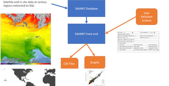
SAVANT exclusion criteria selection. This table represents the following possible exclusion criteria used by SAVANT: (a) satellite box size, (b) maximum time difference between in situ and satellite measurements, (c) maximum observed windspeed and maximum observed aerosol optical thickness, (d) minimum and maximum value of normalized water-leaving radiance, (e) maximum coefficient of variation of satellite box, (f) minimum percent of valid pixels in the satellite box, and (g) additional data quality control flags.
Remotesensing 13 02673 g002
Figure 3. WaveCIS SeaPRISM vs. VIIRS comparison, June 2014–May 2019. Left: permissive protocol; right: strict protocol. The number of match-ups decreased by 65% when applying the strict constraints. Note that in the presented scatter plots there is a black 1:1 line shown for reference purposes, and the colors represent 410, 443, 486, 551, and 671 nm, respectively.
Remotesensing 13 02673 g003
Figure 4. WaveCIS–VIIRS comparison, June 2014–May 2019, center (in situ) pixel only. Left: permissive protocol; right: strict protocol. The number of match-ups decreased by almost 65%.
Remotesensing 13 02673 g004
Figure 5. Venise–VIIRS comparison, June 2014–May 2019. Permissive protocol. Left: 5 × 5 box; right: center pixel only. There is a reduction in some outliers in the 1 × 1 box.
Remotesensing 13 02673 g005
Figure 6. Venise–VIIRS comparison, June 2014−May 2019. Permissive protocol. Left: 443 nm 5 × 5 box mean; right: center (in situ) pixel only. This is the only wavelength in which the 5 × 5 box has statistics closer to the 1:1 line than the center pixel comparison.
Remotesensing 13 02673 g006
Figure 7. Venise–VIIRS comparison, June 2014–May 2019. Strict protocol, left: 5 × 5 box; right: center (in situ) pixel only. The 5 × 5 box is performing closer to the 1:1 line than the center pixel match-ups.
Remotesensing 13 02673 g007
Figure 8. Venise–VIIRS comparison, June 2014−May 2019, 5 × 5 statistical box comparison. Left: permissive; right: strict. There is a 67% drop once again in available match-ups.
Remotesensing 13 02673 g008
Figure 9. MOBY–VIIRS comparison, June 2014–May 2019. Permissive protocol, (a) 5 × 5 statistical box, (b) center (in situ) pixel, and (c) strict protocol. Slightly more than 70% reduction in match-ups from the permissive protocol. Strict 1 × 1 is not presented as the differences are in many cases a few tenths of a percent.
Remotesensing 13 02673 g009
Figure 10. Time series of WaveCIS in situ and satellite match-ups, June 2014 through to May 2019. The highs in both sensors occur during winter time, with spring and summer lows. Also note data holidays caused by the instrument being calibrated or issues at the ground-truth station.
Remotesensing 13 02673 g010
Table 1. Exclusion criteria for the permissive and strict protocols.
ProtocolPermissiveStrict
Box Size5 × 5 and 1 × 15 × 5 and 1 × 1
Time Difference+/−3 h, +/−1 h, +/−0.5 h+/−3 h, +/−1 h, +/−0.5 h
FlagsCLDICE, LAND, ATMFAIL, HILT (processing default)Permissive and HIGLINT, STRAYLIGHT, NAVFAIL, LOWLW
nLw0–30–3
Windspeed≤8 ms−1≤8 ms−1
AOT≤0.2≤0.2
in situ Pixel ValidYesYes
Solar ZenithNot restricted≤75°
Sensor ZenithNot restricted≤60°
Additional RequirementsChlorophyll, all nLw wavelengths validChlorophyll, all nLw wavelengths valid.
Table 2. Strict and permissive results at WaveCIS. June 2014–May 2019 data. Values closest to one in bold, for slope, R2, and mean ratio. Lowest values in bold for bias and mean absolute error.
Protocol/WavelengthMatch-UpsSlopeR2Mean RatioBiasMAE
5 × 5 Permissive @ 410 nm2350.89180.46671.0587−0.0060.1078
1 × 1 Permissive @ 410 nm2360.90120.45621.09390.00170.1093
5 × 5 Strict @ 410 nm820.96720.52511.09210.01060.1108
1 × 1 Strict @ 410 nm840.99570.53481.12010.02140.1074
5 × 5 Permissive @ 443 nm2350.88030.75280.9174−0.05790.1093
1 × 1 Permissive @ 443 nm2360.88420.74230.9377−0.05250.1115
5 × 5 Strict @ 443 nm820.91050.72260.9517−0.03960.1113
1 × 1 Strict @ 443 nm840.91730.71840.9696−0.03160.1096
5 × 5 Permissive @ 486 nm2351.02070.91381.0070.00770.099
1 × 1 Permissive @ 486 nm2361.02170.90381.01690.01090.1054
5 × 5 Strict @ 486 nm821.0410.88951.04360.02590.1089
1 × 1 Strict @ 486 nm841.04670.87341.0690.03770.1142
5 × 5 Permissive @ 551 nm2350.98220.94260.9617−0.02530.0915
1 × 1 Permissive @ 551 nm2360.98260.93140.9693−0.02230.0956
5 × 5 Strict @ 551 nm820.99740.93041.0028−0.00180.0947
1 × 1 Strict @ 551 nm840.99910.91661.02320.0070.1046
5 × 5 Permissive @ 671 nm2350.90070.89190.8586−0.02580.0369
1 × 1 Permissive @ 671 nm2360.89060.86110.8679−0.02590.0389
5 × 5 Strict @ 671 nm820.90570.85580.9142−0.01830.0353
1 × 1 Strict @ 671 nm840.91730.87680.9418−0.01470.0331
Table 3. Venise data, June 2014–May 2019. Permissive data protocol at 5 × 5 and 1 × 1 box sizes. Values closest to one in bold, for slope, R2, and mean ratio. Lowest values in bold for bias and mean absolute error.
Protocol/WavelengthMatch-UpsSlopeR2Mean RatioBiasMAE
5 × 5 @ 410 nm2811.0770.44161.33170.11360.2131
1 × 1 @ 410 nm2801.05780.41561.35670.1090.2181
5 × 5 @ 443 nm2810.99890.77141.07590.0270.1586
1 × 1 @ 443 nm2800.99650.7581.08470.02680.167
5 × 5 @ 486 nm2811.15620.87771.19260.18990.2279
1 × 1 @ 486 nm2801.15250.87081.19550.18970.2331
5 × 5 @ 551 nm2811.04260.90671.06890.060.1258
1 × 1 @ 551 nm2801.0380.91121.07330.06030.1279
5 × 5 @ 671 nm2811.04140.77441.52430.0230.0431
1 × 1 @ 671 nm2801.01610.71491.79370.02470.0482
Table 4. Venise permissive protocol, June 2014−May 2019. Center (in situ) pixel only, at +/−3, 1, and 0.5 h. Values closest to one in bold, for slope, R2, and mean ratio. Lowest values in bold for bias and mean absolute error.
Protocol/WavelengthMatch-UpsSlopeR2Mean RatioBiasMAE
+/−3 h, 410 nm2811.05780.41561.35670.1090.2181
+/−1 h, 410 nm2291.07830.4311.38130.12220.2189
+/−0.5 h, 410 nm1831.05240.37051.35480.11410.2283
+/−3 h, 443 nm2810.99650.7581.08470.02680.167
+/−1 h, 443 nm2291.00080.76331.09660.03570.1664
+/−0.5 h, 443 nm1830.98470.71731.0870.02680.1765
+/−3 h, 486 nm2811.15250.87081.19550.18970.2331
+/−1 h, 486 nm2291.15940.8711.20740.19830.2349
+/−0.5 h, 486 nm1831.15070.841.19950.18950.2405
+/−3 h, 551 nm2811.0380.91121.07330.06030.1279
+/−1 h, 551 nm2291.03690.91021.07710.06130.1227
+/−0.5 h, 551 nm1831.02650.88561.07210.05270.1308
+/−3 h, 671 nm2811.01610.71491.79370.02470.0482
+/−1 h, 671 nm2291.00110.66681.76580.02460.0478
+/−0.5 h, 671 nm1830.85640.47151.75870.01850.0522
Table 5. Venise data, strict protocol. June 2014–May 2019. Values closest to one in bold, for slope, R2, and mean ratio. Lowest values in bold for bias and mean absolute error.
Protocol/WavelengthMatch-UpsSlopeR2Mean RatioBiasMAE
5 × 5 @ 410 nm941.11910.54391.33650.14210.1999
1 × 1 @ 410 nm961.0930.4581.34710.13740.2058
5 × 5 @ 443 nm940.9950.82651.07020.02420.144
1 × 1 @ 443 nm960.99660.78871.07480.030.1563
5 ×5 @ 486 nm941.180.91521.22530.22940.2459
1 × 1 @ 486 nm961.20010.91121.23890.24170.2568
5 × 5 @ 551 nm941.04680.90261.07140.06830.1313
1 × 1 @ 551 nm961.05370.8911.08470.07850.1361
5 × 5 @ 671 nm941.0550.80111.45290.02530.0437
1 × 1 @ 671 nm961.08230.78882.06680.3580.05
Table 6. Venise data, strict protocol. June 2014−May 2019. Center (in situ) pixel only, at +/−3, 1, and 0.5 h. Values closest to one in bold, for slope, R2, and mean ratio. Lowest values in bold for bias and mean absolute error.
Protocol/WavelengthMatch-UpsSlopeR2Mean RatioBiasMAE
+/−3 h, 410 nm961.0930.4581.34710.14210.1999
+/−1 h, 410 nm751.11840.53361.35450.1480.2065
+/−0.5 h, 410 nm611.09790.47641.37320.14840.2192
+/−3 h, 443 nm960.99660.78871.07480.02420.144
+/−1 h, 443 nm750.99110.83221.07450.02290.1433
+/−0.5 h, 443 nm610.97950.80821.07670.01730.154
+/−3 h, 486 nm961.20010.91121.23890.22940.2459
+/−1 h, 486 nm751.17940.92161.22530.22920.246
+/−0.5 h, 486 nm611.1750.92631.22080.22160.2391
+/−3 h, 551 nm961.05370.8911.08470.06830.1313
+/−1 h, 551 nm751.04340.92611.07080.0650.1177
+/−0.5 h, 551 nm611.03940.9281.07370.06180.1112
+/−3 h, 671 nm961.08230.78882.06680.02530.0437
+/−1 h, 671 nm751.03190.77851.45740.02310.0409
+/−0.5 h, 671 nm611.07620.77641.54490.02720.0406
Table 7. Venise 5 × 5 permissive versus 5 × 5 strict. June 2014–May 2019. Values closest to one in bold, for slope, R2, and mean ratio. Lowest values in bold for bias and mean absolute error.
Protocol/WavelengthMatch-UpsSlopeR2Mean RatioBiasMAE
Permissive, 410 nm2811.0770.44161.33170.11360.2131
Strict, 410 nm941.11910.54391.33650.14210.1999
Permissive, 443 nm2810.99890.77141.07590.0270.1586
Strict, 443 nm940.9950.82651.07020.02420.144
Permissive, 486 nm2811.15620.87771.19260.18990.2279
Strict, 486 nm941.180.91521.22530.22940.2459
Permissive, 551 nm2811.04260.90671.06890.060.1258
Strict, 551 nm941.04680.90261.07140.06830.1313
Permissive, 671 nm2811.04140.77441.52430.0230.0431
Strict, 671 nm941.0550.80111.45290.02530.0437
Table 8. MOBY data, June 2014–May 2019. Permissive data protocol at 5 × 5 and 1 × 1 box sizes. Values closest to one in bold, for slope, R2, and mean ratio. Lowest values in bold for bias and mean absolute error.
Protocol/WavelengthMatch-UpsSlopeR2Mean RatioBiasMAE
5 × 5, 410 nm2321.02070.33141.0762−0.01760.272
1 × 1, 410 nm2391.01730.3251.0778−0.02120.2795
5 × 5, 443 nm2320.99940.24681.0430.03430.2194
1 × 1, 443 nm2390.99810.24791.04440.03370.2221
5 × 5, 486 nm2321.02380.07881.0607−0.00520.1328
1 × 1, 486 nm2391.02230.08691.0623−0.00530.1348
5 × 5, 551 nm2320.87430.00020.9738−0.02270.0536
1 × 1, 551 nm2390.86550.0010.9972−0.02210.0584
5 × 5, 671 nm2320.30150.00040.5797−0.01580.0159
1 × 1, 671 nm2390.200800.6233−0.01670.0169
Table 9. MOBY data, June 2014−May 2019. Strict data protocol at 5 × 5 and 1 × 1 box sizes. Values closest to one in bold, for slope, R2, and mean ratio. Lowest values in bold for bias and mean absolute error.
Protocol/WavelengthMatch-UpsSlopeR2Mean RatioBiasMAE
5 × 5, 410 nm680.99830.37271.0538−0.05990.2782
1 × 1, 410 nm690.99530.38561.0409−0.07520.2604
5 × 5, 443 nm680.990.2711.03060.0160.2175
1 × 1, 443 nm690.99020.28911.0220.00960.1987
5 × 5, 486 nm681.00670.08961.0439−0.02670.129
1 × 1, 486 nm690.99750.08161.0307−0.03750.1294
5 × 5, 551 nm680.90420.0150.9947−0.01380.0483
1 × 1, 551 nm690.87390.01531.01−0.01770.0529
5 × 5, 671 nm680.24110.00210.6907−0.01390.0148
1 × 1, 671 nm690.1050.00020.8026−0.01810.0193
Table 10. MOBY data. Permissive versus strict, 5 × 5 statistical box. June 2014–May 2019. Values closest to one in bold, for slope, R2, and mean ratio. Lowest values in bold for bias and mean absolute error.
Protocol/WavelengthMatch-UpsSlopeR2Mean-RatioBiasMAE
Permissive, 410 nm2321.02070.33141.0762−0.01760.272
Strict, 410 nm680.99830.37271.0538−0.05990.2782
Permissive, 443 nm2320.99940.24681.0430.03430.2194
Strict, 443 nm680.990.2711.03060.0160.2175
Permissive, 486 nm2321.02380.07881.0607−0.00520.1328
Strict, 486 nm681.00670.08961.0439−0.02670.129
Permissive, 551 nm2320.87430.00020.9738−0.02270.0536
Strict, 551 nm680.90420.0150.9947−0.01380.0483
Permissive, 671 nm2320.30150.00040.5797−0.01580.0159
Strict, 671 nm680.00210.00210.6907−0.01390.0148
Publisher’s Note: MDPI stays neutral with regard to jurisdictional claims in published maps and institutional affiliations.

