Abstract
Fresh water is a vital natural resource. Earth observation time-series are well suited to monitor corresponding surface dynamics. The DLR-DFD Global WaterPack (GWP) provides daily information on globally distributed inland surface water based on MODIS (Moderate Resolution Imaging Spectroradiometer) images at 250 m spatial resolution. Operating on this spatiotemporal level comes with the drawback of moderate spatial resolution; only coarse pixel-based surface water quantification is possible. To enhance the quantitative capabilities of this dataset, we systematically access subpixel information on fractional water coverage. For this, a linear mixture model is employed, using classification probability and pure pixel reference information. Classification probability is derived from relative datapoint (pixel) locations in feature space. Pure water and non-water reference pixels are located by combining spatial and temporal information inherent to the time-series. Subsequently, the model is evaluated for different input sets to determine the optimal configuration for global processing and pixel coverage types. The performance of resulting water fraction estimates is evaluated on the pixel level in 32 regions of interest across the globe, by comparison to higher resolution reference data (Sentinel-2, Landsat 8). Results show that water fraction information is able to improve the product’s performance regarding mixed water/non-water pixels by an average of 11.6% (RMSE). With a Nash-Sutcliffe efficiency of 0.61, the model shows good overall performance. The approach enables the systematic provision of water fraction estimates on a global and daily scale, using only the reflectance and temporal information contained in the input time-series.
Keywords:
earth observation; landsat; MODIS; remote sensing; probability; Sentinel-2; subpixel; water 1. Introduction
Global freshwater resources are vital for life and our society. Only 2.5% of the earth’s hydrosphere is fresh water [1]. Of this, 0.3% can be found on the surface as lakes, wetlands and rivers. This relatively small fraction is nonetheless highly important, as it constitutes an essential human resource and interacts with climate and biodiversity [2,3,4,5,6]. The quantification of surface water has become a major application in the field of remote sensing, since large and remote regions of interest (ROIs) can be investigated efficiently [7,8]. The utilization of spatial and temporal coherent time-series datasets furthermore offers unique opportunities to analyze variability, dynamics and trends of water bodies [9,10,11,12,13,14]. On a global level, such information can contribute significantly to the understanding of climate change [15] and the effects of human activities [16]. Furthermore, knowledge of water level variations (e.g., by altimetry time-series), in combination with surface water extent dynamics, enables the approximation of waterbody bathymetry, subsequently allowing the quantification of storage change [17,18,19,20,21,22,23]. Thus, essential water variables can be monitored, providing key indicators for the implementation of sustainable development goals [24].
A variety of methods to distinguish between water and non-water surfaces have been developed in recent years. For instruments working within the range of RADAR (radio detection and ranging) frequencies, generally a weaker backscatter signal can be expected from water surfaces in comparison to most land surfaces [25,26,27]. RADAR-based sensors have the advantage of being widely unaffected by atmospheric conditions (e.g., cloud cover, water vapor, aerosols). However, increased roughness of an open water surface can lead to stronger return pulses. In addition, land features of low backscatter similar to smooth water (e.g., bare grounds, RADAR shadow, sand dunes) are prone to misclassification [25]. In the optical domain, emphasis is given to visible (VIS), near infrared (NIR) and shortwave infrared (SWIR) channels for classification, as water shows stronger absorption in these wavelength ranges than typical land features [13,21,28,29,30,31,32,33,34,35,36,37,38,39,40]. However, the accurate mapping of waterbodies is a non-trivial task, even on the basis of multispectral data [41]. Land objects such as urban areas, volcanic materials, coal mines, burned areas as well as cloud- or relief-induced shadows show similar reflectance properties as water surfaces [31,37,42,43]. The spectral signature of water pixels is furthermore altered by water depth and corresponding ground materials or contamination by hydrosols (e.g., sediments, aquatic vegetation) [13,31,44,45]. Mixed pixels (water, non-water) also create an altered spectral response, depending on the fractional occurrence of endmember surfaces [46,47]. Relatively small waterbodies or continuous water-land boundaries can intensify this effect, especially when operating on coarse resolution images [48]. When targeting temperature differences (thermal infrared) between water and non-water surfaces, results are strongly dependent on prevalent weather and landcover conditions [49,50]. Furthermore, temporal diversities such as sun-sensor geometry and atmospheric conditions complicate the generation of consistent time-series [31,45,51,52,53]. Especially for optical data, atmospheric distortions (e.g., clouds, dust particles) influence radiation transfer and might result in invalid observations for affected pixels and regions, thus reducing the temporal integrity of a remote-sensing time-series.
According to dataset characteristics, specific applications are suitable. For instance, static datasets provide information on the spatial extent of water bodies for specific points in time, aggregations of longer time periods, or combinations from different sources [54,55,56,57,58,59,60,61]. In these cases, water surfaces are related to timely persistent (≥1 year [62]) land cover. In addition, several general-purpose land-cover datasets contain water classes [63,64,65]. Alternatively, a focus on rather rapid temporal changes (≤ 1 month) between land and water states is able to reveal the dynamics of water bodies [10,13,33,66,67,68,69,70]. Typical applications are inundation [44,71,72] or near-real-time (NRT) flood monitoring [73,74,75]. As changes in water surface extent can occur in different time scales, rapid changes might be missed by monthly composites or relatively static annual averages [13,14,31,76]. In addition, investigations focusing on the timing of hydrological events [77] require high temporal resolution. An additional advantage of high temporal resolution is the avoidance of the spatiotemporal inconsistencies of other models or remote sensing datasets (e.g., water budget estimation [7]).
By targeting daily information on the distribution of water surfaces on a global level, several optical sensors featuring medium spatial resolution can be considered. These include the Moderate Resolution Imaging Spectroradiometer (MODIS), Visible Infrared Imaging Radiometer Suite (VIIRS), Ocean and Land Colour Instrument (OLCI) and Advanced Very-High-Resolution Radiometer (AVHRR) [31]. Among these, MODIS has the advantage of long-term (2000–present) uninterrupted lifetime sensors with an onboard calibration system.
Water fraction estimation has been applied frequently to resolve coarse spatial resolution problems when quantifying surface water [29,34,78,79,80,81,82,83]. The identification of the relative water and non-water content of a coarse pixel becomes increasingly relevant for applications sensitive to the accuracy of areal estimations and their change dynamics (e.g., rapid inundation changes). Typically, related applications are limited to distinctive sites and have not been applied to comprehensive time-series data. This may be owing to the requirement of prior knowledge concerning target regions (e.g., land cover, a priori water/non-water state, elevation, endmember definition and samples for learning algorithms) in order to apply subpixel methods [78,82,84]. This includes machine learning techniques (e.g., decision trees [34], regression tree models [84], Gaussian Process Regression model [83]) used for water fraction estimation. Thus, the constraint of training samples for model building limits applications to distinct sites. In addition, neural networks have been applied for water fraction estimation [85], facing similar constraints as machine learning approaches. By implementing additional data (e.g., topographic, hydrographic data [60]), the downscaling of coarse resolution images to a finer resolution is possible. Limitations to downscaling techniques are due to the quality of original observations and ancillary data. A further technique is the fusion of moderate- and high-resolution images [86]. However, fusion techniques rely on the underlying assumption of spatiotemporal continuity, which is not given for rapid changes. Many applications feature unmixing methods to estimate water fraction, mainly based on the utilization of a linear mixture model [29,34,42,81,87]. Such approaches rely on the assumption that remotely sensed reflectance of a mixed pixel can be expressed as a linear combination of spectral endmembers. Linear spectral mixture modeling is often applied to hyperspectral data to determine the relative abundance of predefined endmembers. A constraint is given by the prerequisite of a priori endmember definition, which is critical for accurately extracting the fraction of endmembers [88]. Furthermore, a sufficient number of bands is necessary to solve decomposition equations [81]. For the global and systematic application of a linear mixture model, two constraints need to be considered [81,83]. Global endmembers have to be defined dynamically in space and time; otherwise, they are not representative. Additionally, the number of bands provided should be larger than the number of endmembers. MODIS only provides two bands at 250 m resolution; consequently, a rather simple and robust model has to be considered.
In this paper, we aim to systematically derive water fractions on pixel level, to improve the quantification capabilities of a MODIS-based earth observation time-series for inland surface water [31]. To achieve this in a consistent spatiotemporal manner, water fraction is estimated on the basis of classification probability and spatial pixel relations, including temporal coherences. Furthermore, we evaluate the optimal configuration of input features and parameter settings for the global utilization of a linear mixture model [89]. The performance of resulting subpixel water fraction estimates is assessed by comparison to reference data gained from classified higher resolution optical data (Sentinel-2 and Landsat 8). Finally, we show that water fraction estimates are able to enhance quantitative capabilities concerning mixed pixels.
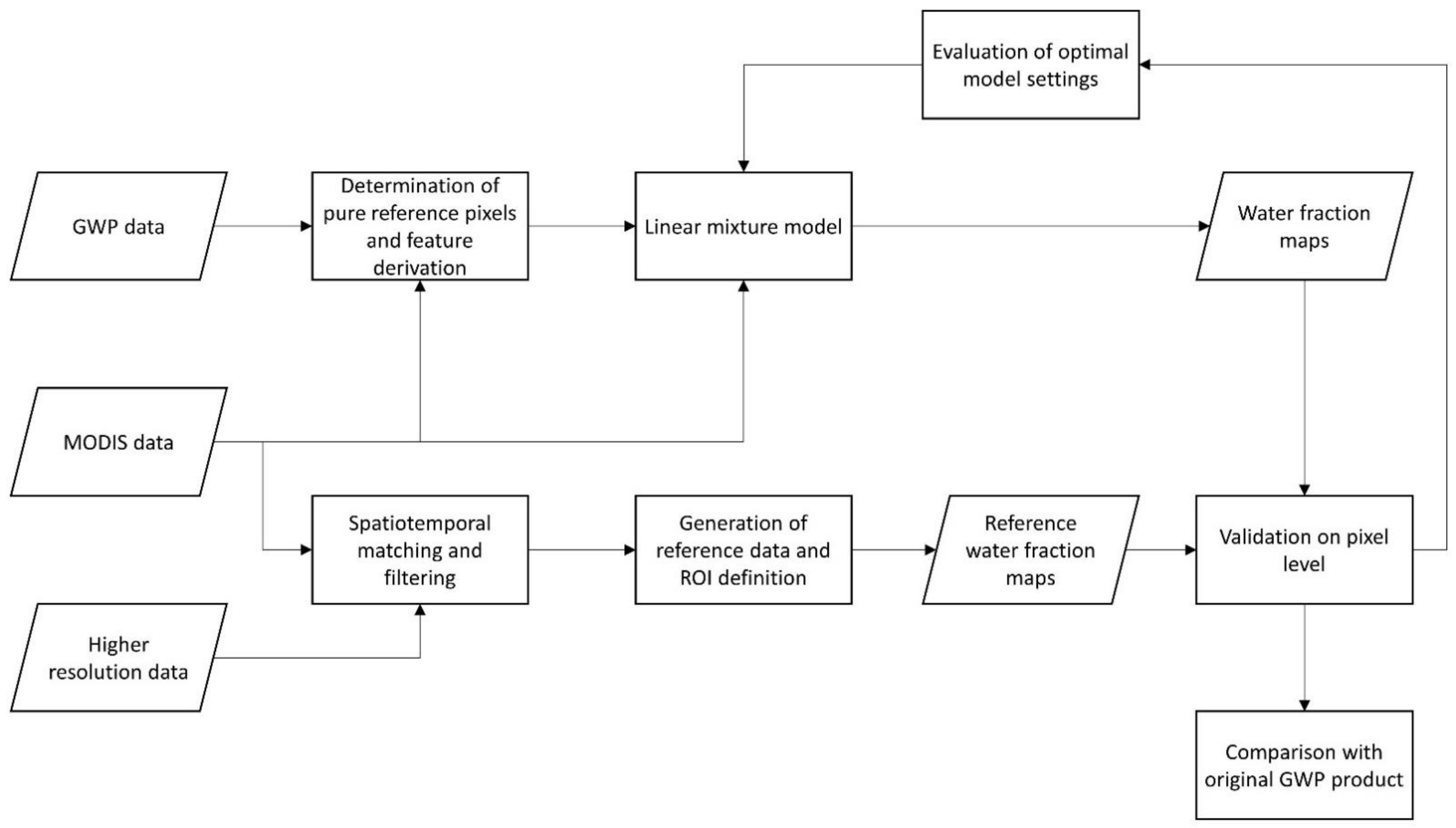
2. Materials and Methods
For this study, we use reflectance data from MODIS, GWP water/non-water classifications, and higher resolution optical images (Landsat 8 and Sentinel-2) as input data. Input features for the linear mixture model are determined from GWP time-series information and MODIS RED and NIR reflectance. Generated water fraction maps are evaluated utilizing reference data gained from higher resolution remote sensing images. By comparison of model performance using different model parameters, the optimal setting considering all reference data is determined. Outcomes of the final model are then evaluated together with the original GWP time-series on pixel level (Figure 1).
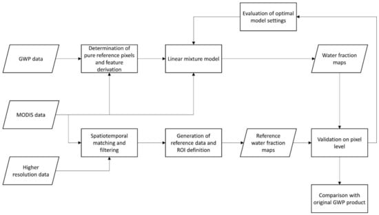
Figure 1.
Workflow of the proposed method to systematically derive water fractions.
2.1. Data
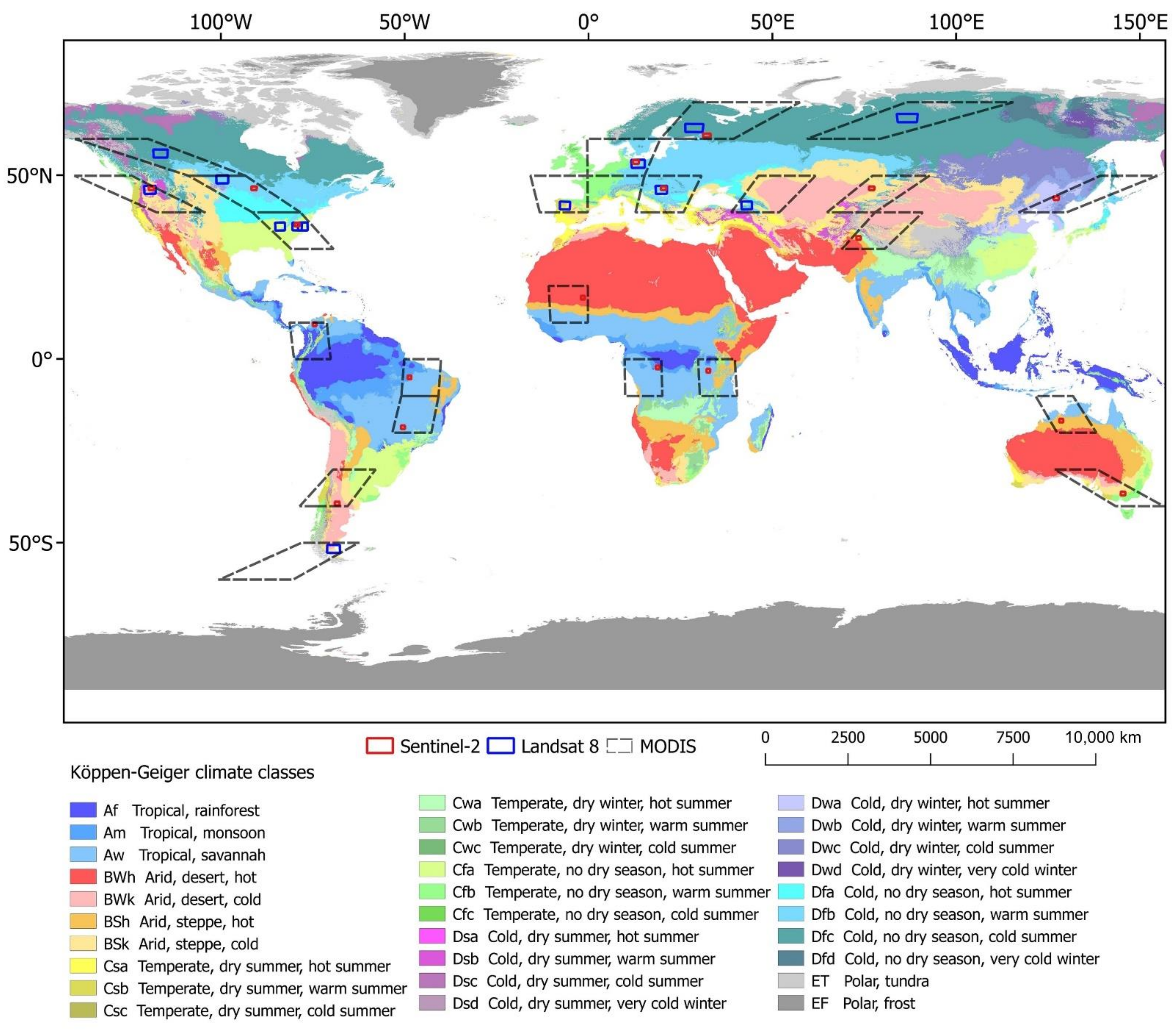
The Global WaterPack (GWP) inland surface water time-series is based on bi-diurnal moderate resolution acquisitions of MODIS sensors Aqua (MYD09GQ) and Terra (MOD09GQ). A binary water mask is created in a dynamic thresholds-based procedure, utilizing NIR and NIR-RED band reflectance. Additionally, several auxiliary layers (multi spectral information, day-night difference, urban areas, relief shadows, thermal information) are used to refine classification output and mask clouds and ocean (MODIS MYD10A1, MOD10A1). To create a temporally consistent time-series, data gaps (mostly due to cloud cover) are interpolated by a moving window approach, which utilizes the closest past and future valid observations of a pixel. For this paper, we use GWP data of 23 MODIS tiles in conjunction with 32 spatiotemporal matches of higher resolution reference datasets. Suitable reference surface reflectance images are selected from Sentinel-2 (Level-2A) and Landsat 8 (OLI/TIRS Level 2) archives. For this study, ROIs are defined by intersections of MODIS tiles and selected Sentinel-2 /Landsat 8 tiles, which spread across different continents and climate zones to represent global variability (Figure 2).
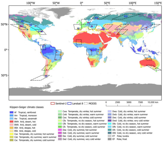
Figure 2.
Global distribution of regions of interest (ROIs) and climate classes [90].
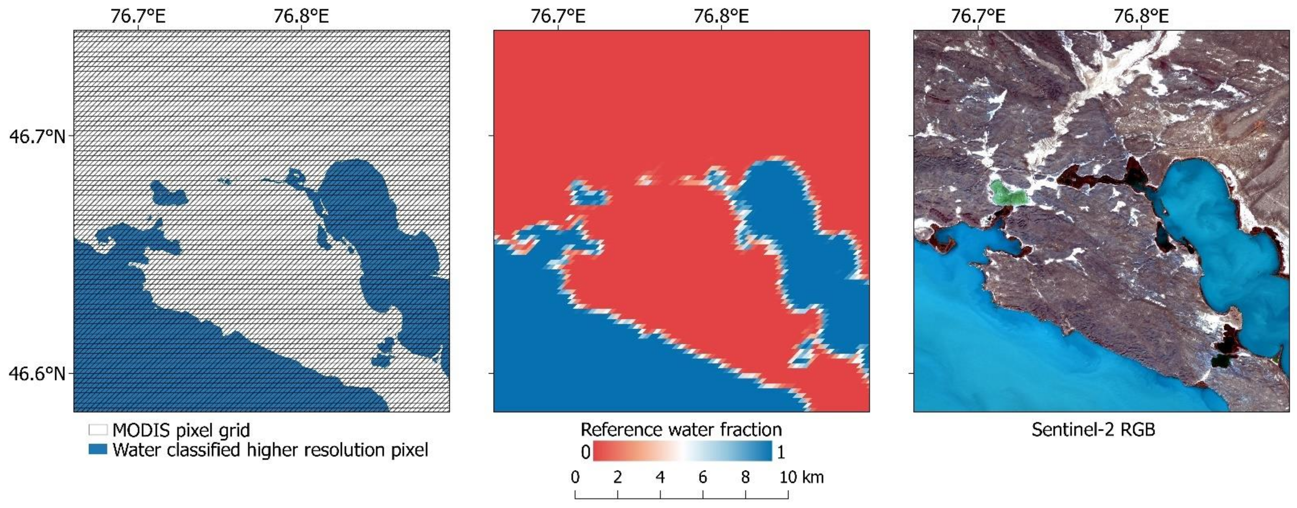
2.2. Generation of Reference Data
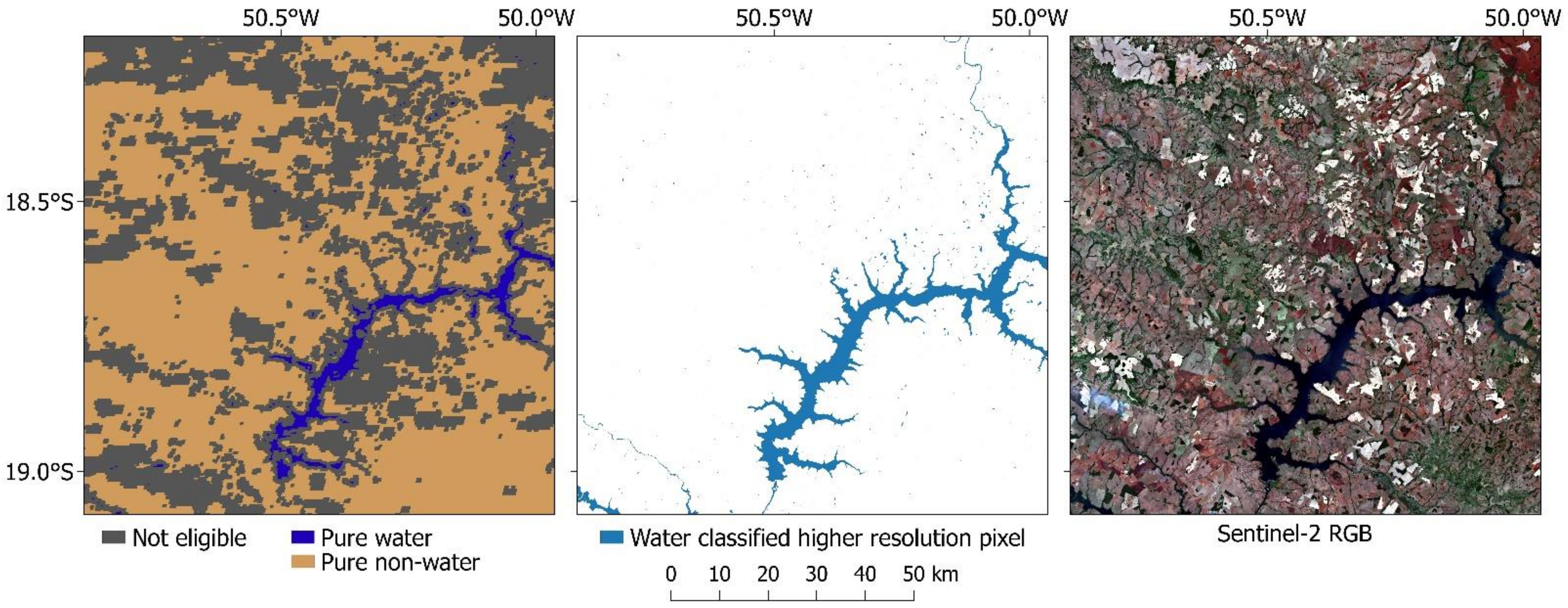
Reference data was generated based on Sentinel-2 and Landsat 8 images (Table A1). Spatiotemporal matches with MODIS data were selected, considering global distribution and data integrity (low cloud coverage (<1%) and completeness). Accordingly, a selection of 32 remote-sensing image pairs enabled the generation of approximately 622,900 km2 of reference area (15,260,357 reference pixels). Consequently, a wide range of surface cover compositions accounted for method sensibility to variable surface reflectance properties. Higher resolution (30 m for Landsat 8, 10 m for Sentinel-2) water/non-water masks were generated by k-means segmentation [91,92] as well as tasseled cap transformation [93]. After unsupervised classification, all reference images underwent rigorous visual verification to ensure data quality. Subsequently, higher resolution water pixels were allocated to a larger MODIS pixel, in case their pixel centers intersected. To minimize projection related errors in the spatial matching of pixels, a MODIS pixel grid vector version was reprojected from sinusoidal projection to the according spatial reference system of the reference image. Finally, reference water fraction was determined by the ratio of allocated higher resolution water and non-water pixels (Figure 3).
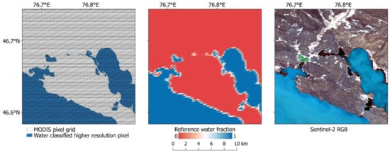
Figure 3.
Allocation of classified Sentinel-2 reference pixels to larger MODIS pixels to gain reference water fraction estimates. Data: Sentinel-2 tile R048 T43TFM, 2019-10-23.
Furthermore, a reference water fraction pixel is only valid if the accumulated pixel area of allocated higher resolution pixels amounts to at least 95% of the MODIS pixel area (~59,375 m2).
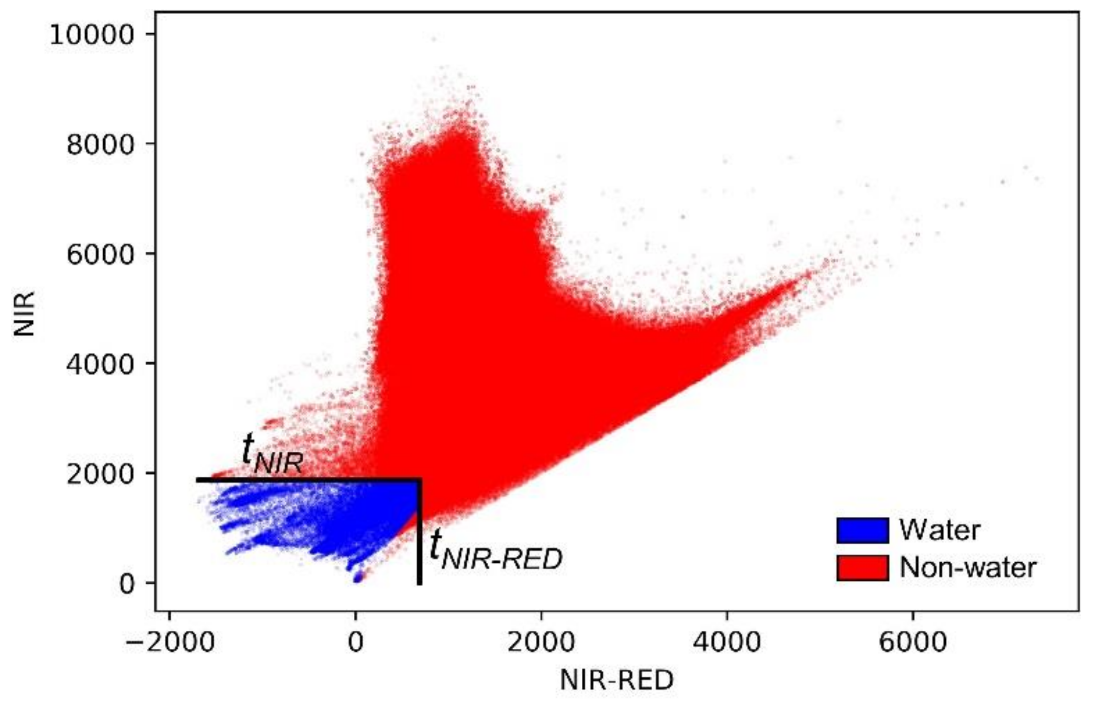
2.3. Classification Probability
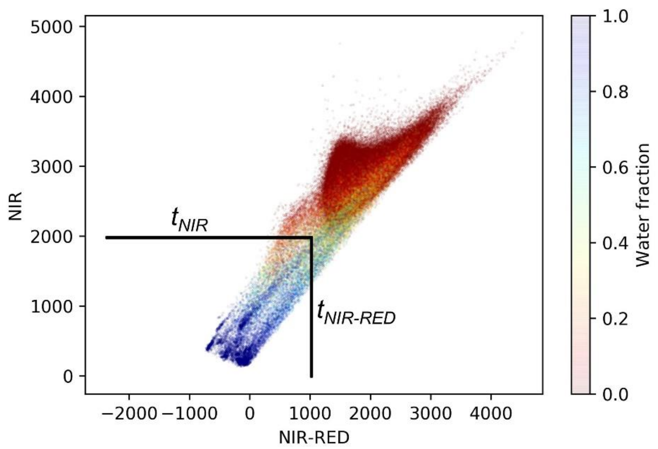
The classification probability of a remote-sensing product depends on the classification methodology (e.g., fuzzy or soft classification). To determine the classification probability of GWP, relative datapoint locations in feature space were utilized. For every daily GWP classification of sensor-specific data (MODIS Aqua and Terra), two thresholds (tNIR and tNIR-RED) were derived from known water pixels. These water pixels were selected in the original product based on additional tile-specific information from MOD44W (MODIS Terra Land Water Mask) and MOD10A1/MYD10A1 products [31]. The resulting distribution of NIR and NIR-RED values within training areas allowed the determination of daily thresholds. To minimize the day-to-day noise, eventually an 8-day-mean temporal filter was used for smoothing. Accordingly, water and non-water pixels were discriminated based on NIR and RED reflectance. For GWP, classification probability relates to the distance between pixel data points and scene-specific dynamically derived thresholds in the NIR and NIR-RED feature space (Figure 4).
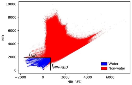
Figure 4.
GWP classification feature space. Data: MODIS Terra h17v07, 2019-10-22.
2.4. Linear Mixture Model for Water Fraction Estimation
To facilitate systematic water fraction estimation, the linear mixture model of Sheng et al. [89] was utilized. Accordingly, the reflectance of a mixed pixel (Rmix) for VIS to SWIR wavelengths could be estimated by its fractional water coverage (WF) and the approximated reflectance of pure water (Rwater) and non-water (Rnon-water) pixels:
solved for WF,
where
Since this method was applied to Aqua and Terra data separately, outcomes were combined based on spatial data availability. By using information from both MODIS sensors, generally a higher quality of outcomes could be expected (e.g., MODIS Nadir Bidirectional Reflectance Distribution Function (BRDF)-Adjusted Reflectance dataset MCD43A4 [70]). Thus, in case both sensors were able to provide surface reflectance information for a pixel, the average of model outputs was used; otherwise a single estimate depicted the combined result. The number of included sensors (one, two or none) was stated in an additional reliability band of the output raster.
2.5. Feature Selection
R predictor variables in the linear mixture model can be substituted by specific features related to reflectance [34]. Aspiring to model application on a global level, we tested a variety of input parameters to determine the optimal setting, considering all ROI datasets (Figure 1). As proxies for Rmix, Rwater, and Rnon-water, eight features based on MODIS reflectance and GWP classification thresholds were derived (Table 1):

Table 1.
Input features for the linear mixture model.
For feature selection, significant linear correlation (r > 0.5, p < 1%) in the majority of ROIs to known reference water fraction was a precondition. An example for a typical distribution of pixel data points with given reference water fraction is shown in Figure 5.
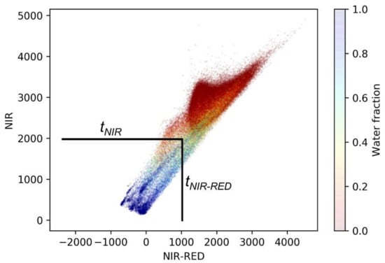
Figure 5.
Pixel data points (based on MODIS reflectance) with reference water fraction information (based on Sentinel-2) and GWP classification thresholds. Data: MODIS Terra tile h10v08 and Sentinel-2 tile T18PWR, 2019-02-08.
For application in the linear mixture model, features are expected to show lower values for water than for non-water pixels and vice versa. Consequently, distance features are signed negative for pixels in the GWP water classification window (area beneath tNIR and left of tNIR-RED, Figure 4 and Figure 5).
2.6. Selection of Pure Pixel Reference Features
To enable a systematic approximation of pure water and non-water features (Rwater and Rnon-water) we utilized spatial pixel relations and temporal information contained in the time-series. Pure water pixels are typically part of larger coherent waterbodies. According to this spatial relationship, a pixel that has water-covered neighbors is likely to contain pure water coverage itself. The same principle applies for the determination of pure non-water pixels. By considering the 8-pixel neighborhood of an evaluation pixel in the center, pure pixel candidates were evaluated. As optical MODIS observations are often rendered invalid by cloud coverage, we also determined monthly and yearly temporal averages (TAs) based on future and past observations of the evaluation pixel. For this, the ratio of classified water and valid observations for monthly (±15 days) and yearly (±182 days) temporal windows was calculated to yield water probability (pw). To also consider the reliability of averages, the ratio of valid observations and temporal window length (rw) was determined. Consequently, invalid observations in the pixel neighborhood were primarily substituted with monthly TA, given a valid observation in the monthly temporal vicinity. Otherwise, the yearly TA was used (Figure 6):
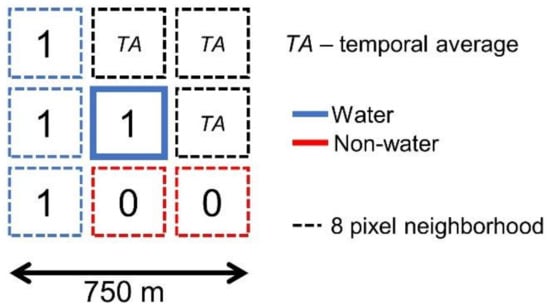
Figure 6.
Spatiotemporal relations based on neighborhood pixels. Here, three observations are invalid and therefore substituted by temporal averages (TAs).
Finally, a purity probability (pp) and reliability (pr) were determined by averaging of all n pixels in the neighborhood as well as the center pixel:
Hereby, valid water or non-water observations contributed with 100% or 0% probability, respectively, and 100% reliability. Subsequently, pixels could be considered as pure if several criteria were met. First, pure water candidate pixels must exhibit a pp of 100% (completely surrounded by neighboring water pixels), with a pr value of at least 95%. Conversely, pure non-water pixels had to show a pp of 0%. Furthermore, only pure pixels that had been classified as water or non-water based on a valid observation on the respective day were selected (Figure 7).
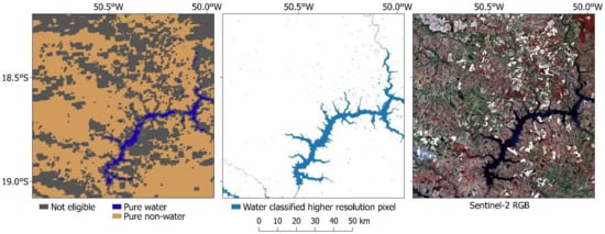
Figure 7.
Selection of pure water and non-water pixels. Data: MODIS Terra tile h13v10 and Sentinel-2 tile R081 T22KEE, 2019-10-15.
Based on this pure pixel selection, samples for typical water/non-water feature values (Table 1) were derived. Subsequently, respective reference statistics, including mean, median, 75th and 25th percentile were determined from these sample feature values. By utilizing different numerical measures, more modest (25th percentile), optimistic (75th percentile) and balanced (mean, median) water fraction estimates were available for evaluation.
2.7. Performance Evaluation and Determination of Optimal Settings
Water fractions were evaluated on pixel level in 32 ROIs (Figure 1). Results for respective combinations of features and reference feature statistics were evaluated by determining Pearson’s correlation (r), root mean square error (RMSE) and mean absolute error (MAE) with regard to reference data:
where e is the difference between model estimate (x) and reference water fraction (y), and n is the number of data points.
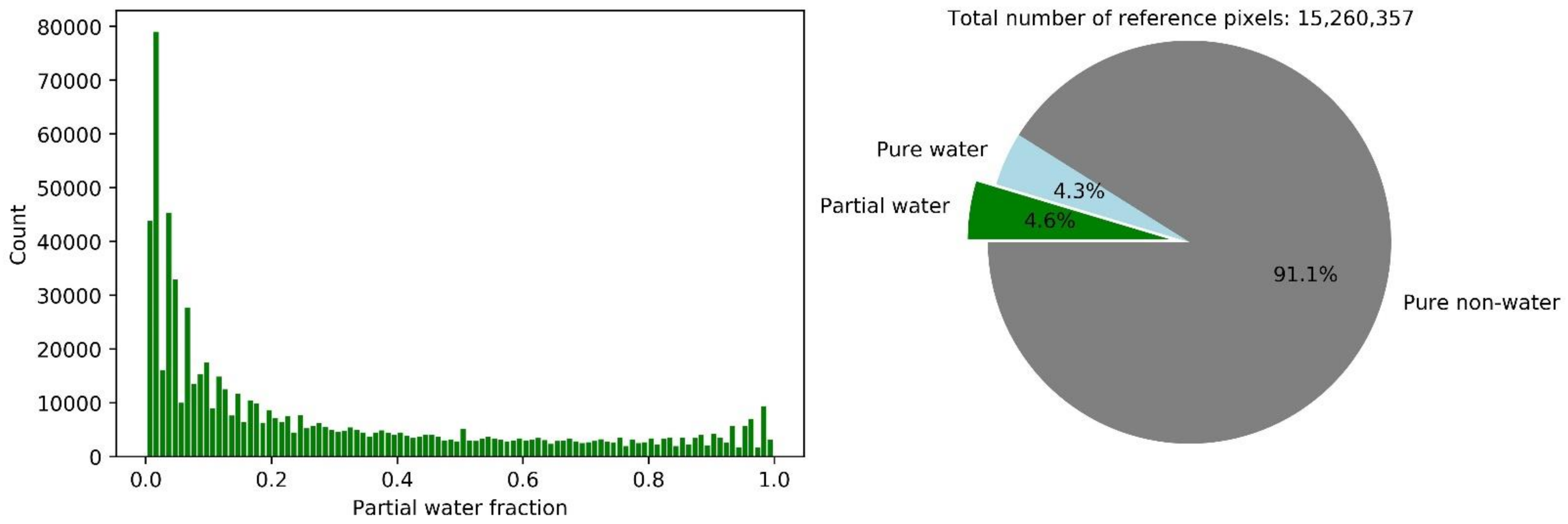
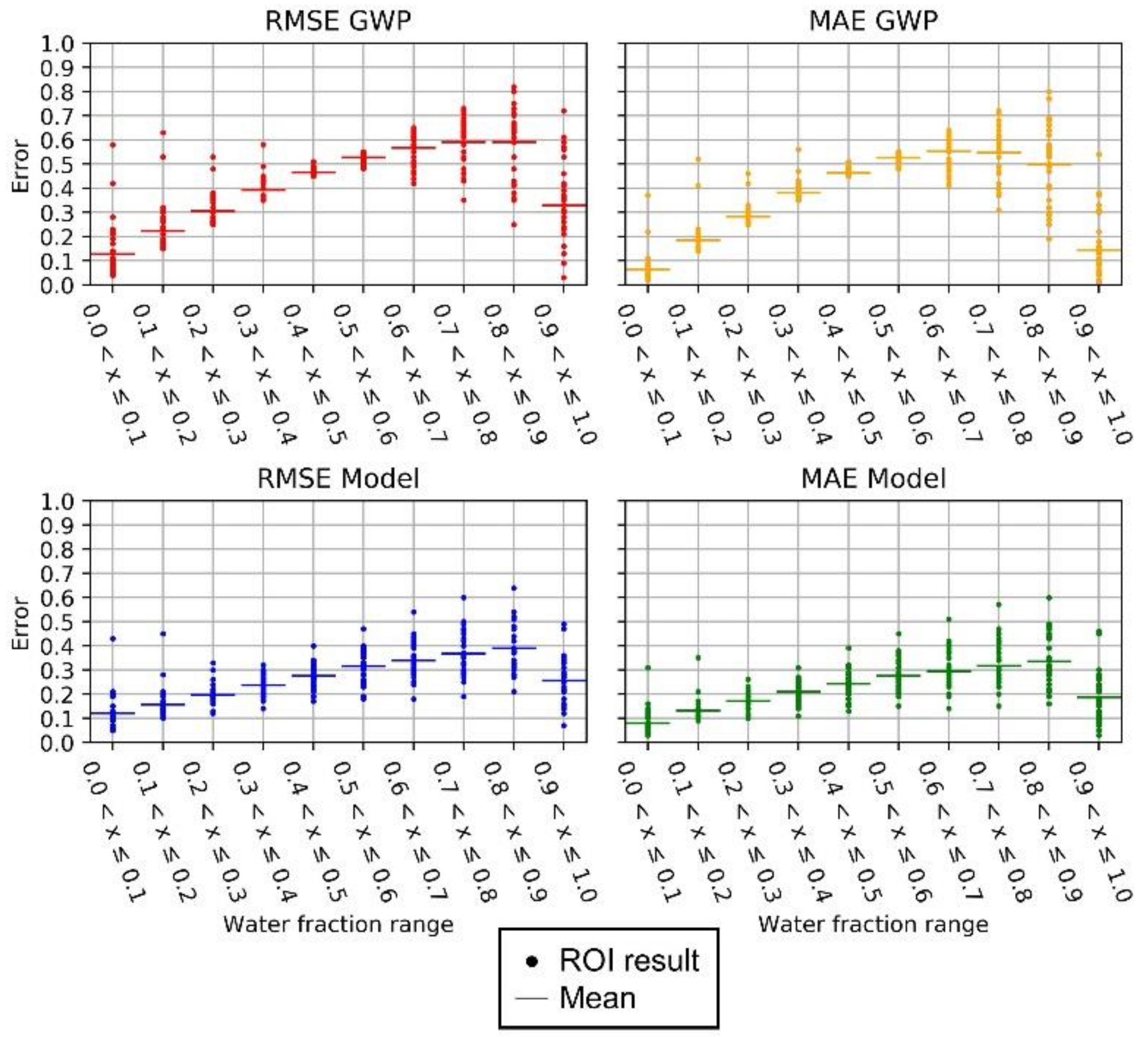
We chose two error metrics to further investigate error distribution. While the MAE gives the same weight to all errors, the RMSE penalizes higher variability in the distribution of error magnitudes by assigning more weight to larger error values [94]. Typically, the majority of pixels in an ROI exhibit no water coverage, biasing evaluation metrics towards zero-water fraction conditions. To reveal coverage-specific performance, we grouped spatiotemporal matches of model output and reference data in pixel coverage categories. Thus, separate assessments were conducted for reference pixels showing full water coverage, no water coverage and partial water coverage (0% < x < 100%). The distribution of all generated reference pixels is shown in Figure 8:
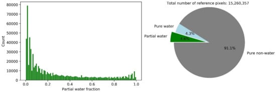
Figure 8.
Distribution of reference pixels according to coverage categories. The histogram shows only partial water fraction pixels (0% < x < 100%).
To determine the best performing model configuration for respective coverage categories, all ROI-specific outcomes per MODIS sensor were averaged.
2.8. Evaluation According to Water Permanence Types
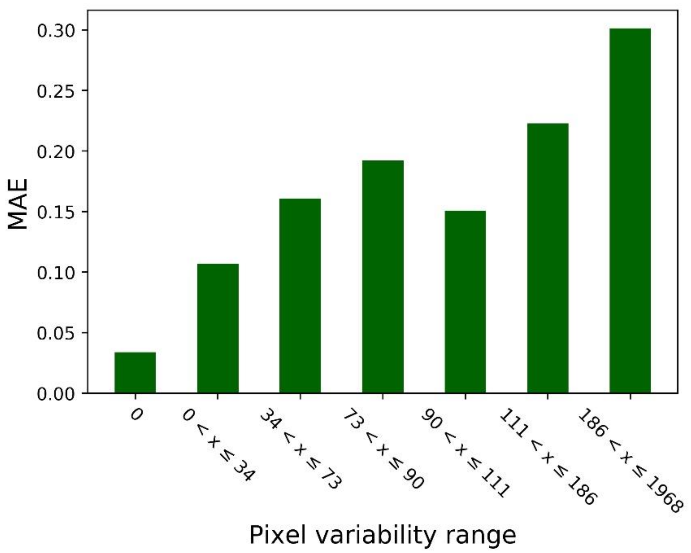
To assess the influence of pixel cover permanence on model performance, we determined the number of pixel state changes between water and non-water. This was conducted based on the GWP time-series for a time span of 6575 days (2003–2020). The resulting pixel variabilities of all pixels in the ROIs were grouped according to variability percentiles. Therefore, each selected variability range represents 1% of the available data, except the zero percentile (permanent pixels), which includes 94% of the data. Finally, the MAE of the respective model estimates and reference water fractions provides information on the influence of pixel change behavior on model performance.
3. Results
Best performing settings and corresponding results (lowest RMSE/MAE, highest correlation) are shown in Table 2.
Table 2.
Optimal parameter settings for pixel coverage categories.
The global evaluation showed that each coverage category favors a specific parameter setting. As most of the data is constituted by pure non-water pixels, the optimal setting for all data is biased towards this coverage category (distance threshold point feature and 25th percentile reference statistic). Larger errors occur in the partial coverage category, whereas pure pixel coverage can be approximated more accurately (average of 13% lower error).
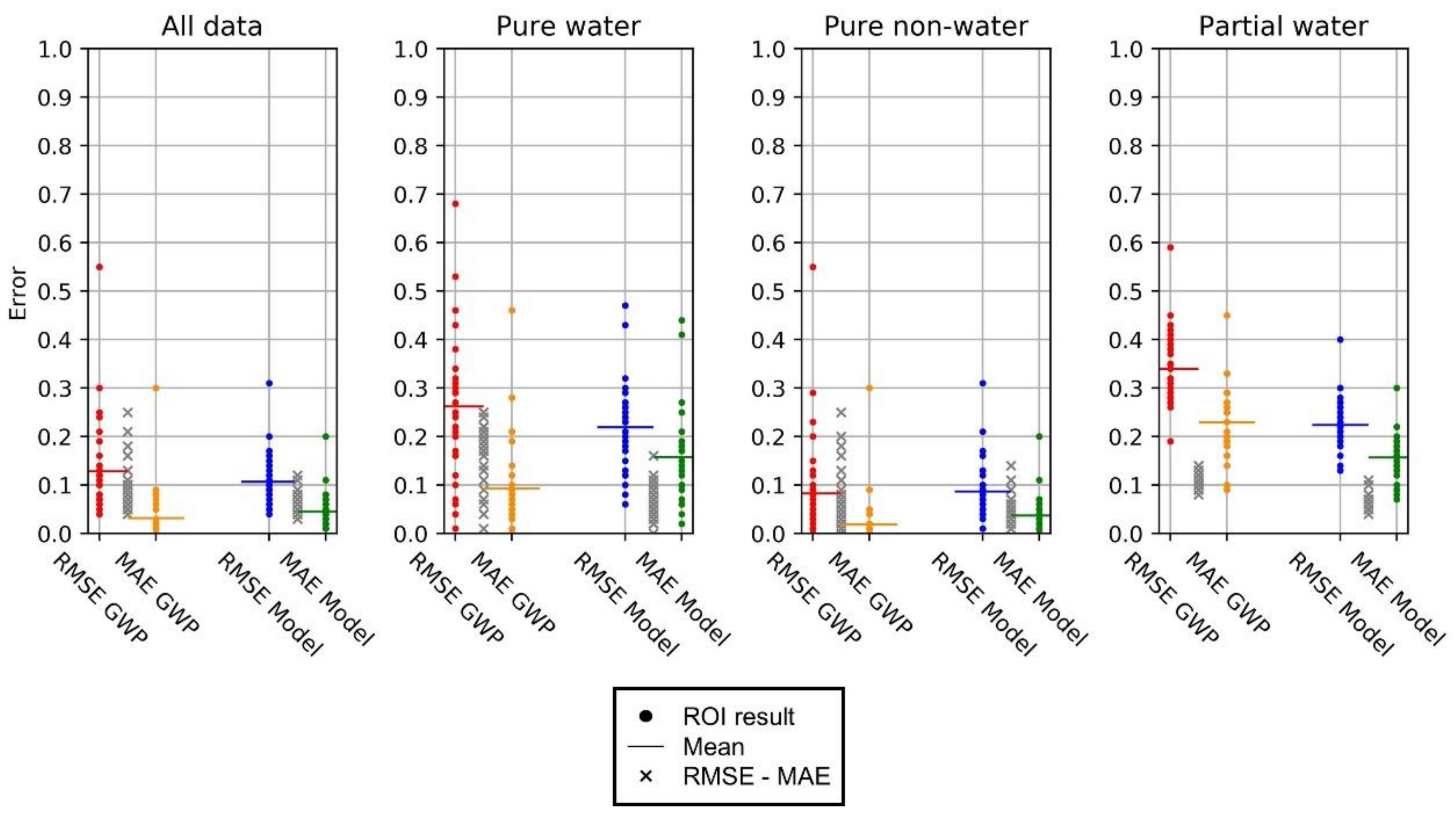
Using the optimal settings for all data (distance to threshold point, 25th percentile), we evaluated model output together with raw (without refinement by auxiliary layers) binary GWP classifications (Figure 9).
Figure 9.
Model and GWP performance according to coverage categories for all ROIs.
The comparison shows higher accuracy of water fraction model estimates for pixels with partial water coverage. For entirely water or non-water covered pixels, binary GWP classifications average to lower MAEs than model estimations, as only falsely classified pixels lead to errors in pure pixel categories. The water fraction model tends to underestimate surface water in the pure water category (average of 16% MAE), and to a smaller extent overestimates water coverage for pure non-water reference pixels (average of 4% MAE). Differences between ROI-specific RMSE and MAE error statistics indicate a generally smaller variance in the distribution of error magnitudes for model estimations than for GWP. This is caused primarily by rare GWP misclassifications of pure pixels, which result in large outlier errors of 100%. Model and GWP performance in the partial water category is dependent on the ratio of pixel water and non-water coverage (Figure 10).
Figure 10.
Model and GWP performance in all ROIs for specific intervals of partially water-covered pixels.
Larger errors in GWP were found for pixels with a balanced water/non-water ratio, whereas model estimates show lower accuracy for nearly full pixels (0.8 < x ≤ 0.9 water fraction). A general skewedness towards low water fraction indicates a more reliable approximation of minorly water-covered pixels.
To assess the goodness of fit of the proposed approach, we also determined the Nash-Sutcliffe efficiency (NSE), percent bias (PBIAS) and RMSE, considering all datapoints given by the reference data.
A NSE of 0.61 indicates a generally good match between model and reference data [95,96]. With a negative PBIAS of −62.34%, the model tends overestimate actual water fraction [97]. The total RMSE of 0.11 indicates a good overall performance, considering a standard deviation of 0.19 of all reference water fractions [98]. The evaluation according to water permanence types showed larger MAEs for change-intensive pixels than for more permanent ones. In the range of moderate pixel variability (34 to 186 state changes in 6575 days), only minor differences in model performance can be observed. Figure 11 shows MAEs for pixels in specific pixel variability ranges, based on variability percentiles.
Figure 11.
MAEs of model estimates and reference data for specific pixel variability (x) ranges representing 1% of all available data, except the zero percentile (94% of the data).
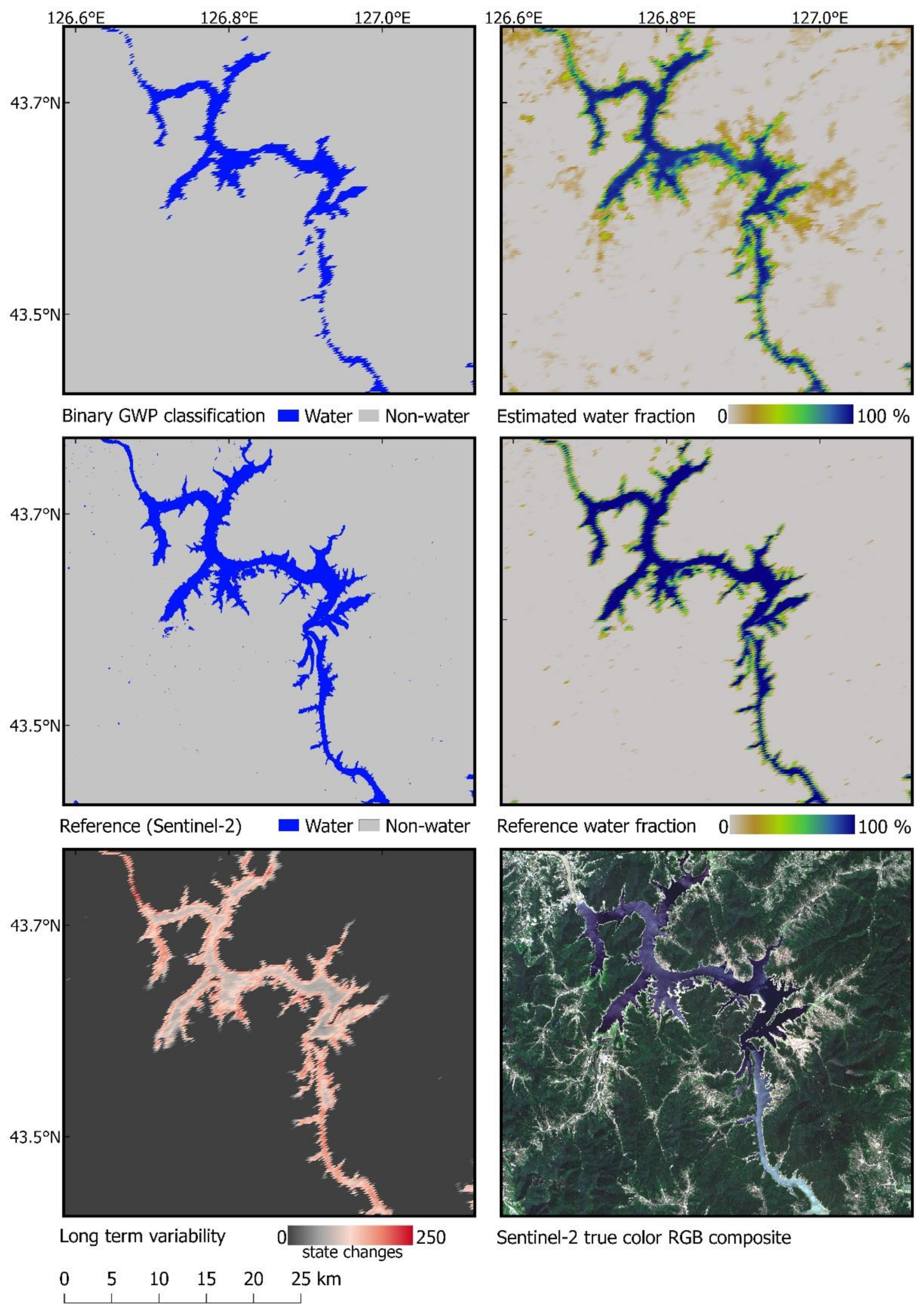
To illustrate the improvements achieved by water fraction estimation, Figure 12 shows a comparison of original GWP and higher resolution water masks, model and reference water fractions, as well as corresponding variability and true color information for the Songhua Lake and River.
Figure 12.
Comparison of original GWP binary classification, estimated water fraction and reference water fraction based on Sentinel-2 for Songhua Lake and River (China) on 2019-07-10. Water variability refers to the 10-year time-series of MODIS tile h27v04 and illustrates typical extent variations.
4. Discussion
For geospatial raster datasets such as GWP, total surface water extent can be approximated by accumulation of water-classified pixels. Limitations given by the moderate spatial resolution of a product induce quantification errors. A single pixel in the highest spatial resolution of MODIS accounts for approximately 62,500 m² of classified area. Accordingly, relatively coarse spatial resolution results in discrete areal quantification steps for the estimation of the actually continuous extent of waterbodies such as lakes, reservoirs or rivers. This can lead to erratic changes in estimated surface water extent, given a change-pixel constitutes a relatively large part of a study site or waterbody. Furthermore, subpixel-scale water extent variations are able to move respective mixed pixel data points just across classification threshold boundaries, thus overemphasizing actual extent changes. As a consequence, derived temporal behavior can be misleading. The extent to which this affects estimations of total surface water area strongly depends on the investigation scale and waterbody characteristics. Accordingly, water fraction estimates become increasingly relevant if extent changes are a matter of small-area variations (few pixels to subpixel scale, e.g., shoreline pixels of relatively stable waterbodies).
We showed that by considering GWP classification probability and spatiotemporal time-series information, subpixel water fractions can be approximated in an automated fashion. Accordingly, subpixel-scale water or non-water surfaces are accounted for; they otherwise would be disregarded. Especially for waterbodies with jagged shoreline characteristics (large shore-to-area ratio) as shown in Figure 12, the approach enables an enhanced estimation of surface water extent compared to binary classification.
To accurately capture the distinct temporal extent dynamics of highly variable waterbodies (e.g., dam regulated reservoir), the residual water or non-water fraction of change-intensive shoreline pixels (Figure 12, left bottom) must not be neglected. Therefore, the presented approach enables a systematic provision of water fraction along with the product’s spatiotemporal extent. Nonetheless, several arbitrary factors influence model accuracy. Since the relative pixel location in the NIR/NIR-RED feature space mainly determines its water fraction content, surface types with similar spectral properties in respective wavelengths can lead to an overestimation of water fraction (e.g., urban areas; Figure 12, top right). However, as problematic surface types are already masked by auxiliary layers in GWP, the handling of overestimations caused by urban areas, cloud shadows, burned areas or relief shadows is straightforward. On the other hand, water properties such as depth, in conjunction with ground materials, turbidity and vegetation content, can corrupt water fraction estimation. The other variable parameters in the linear mixture model are the feature reference values for pure water and non-water pixels. As they are determined from a selection of reference pixels, derived values per scene are dependent on the availability (e.g., by cloud cover location) and the current state (e.g., land cover type phenological state) of these pixels. Nevertheless, information for the determination of model input data is collected dynamically in time from a respective large-area MODIS tile. Consequently, the approach is robust to certain randomness, as a relatively large amount of pure pixel reference information is used to derive model parameters. If certain applications demand surface water estimation in more detail, a customization of model settings for specific tiles or even smaller ROIs is feasible. Similar strategies, along with the use of auxiliary data, have led to highly accurate applications in previous studies [29,34,81,82]. The effect of different model settings on the performance regarding specific pixel coverage categories can be seen when comparing the error scores of Table 2 and Figure 9. Here, better results can be achieved in pure water and partial water coverage categories if other parameter settings are chosen than the optimal setting for all data.
The comparison to reference water fractions derived from higher resolution data showed that the proposed model is able to improve quantification accuracy of the product. This results in a better approximation of the true water coverage of mixed water/non-water pixels. Consequently, the ability to estimate residual contents in otherwise binary classified pixels is gained. The extent to which this improves the accuracy of surface water estimations depends on the relative area of partially water-covered pixels in an ROI, as well as the coverage ratio of those pixels (Figure 10). Thus, applications focusing on known waterbodies and their areal dynamics in time benefit from more comprehensive consideration of mixed shoreline pixels (Figure 12). The evaluation of optimal settings resulted in a modest (25th percentile reference statistic) approach, which promotes the estimation of minorly water-covered pixels (Figure 10). Although GWP surpasses model performance in pure pixel categories (Figure 9) considering MAE, larger RMSEs on the other hand suggest that the distribution of error magnitudes is more variable. Consequently, model estimations can be expected to not feature as extraordinarily large errors in single cases as GWP.
The evaluation of model performance according to water permanence types showed that higher error occurs for pixels that change their water/non-water state more frequently (Figure 11). As the model accuracy is generally higher for pixels exhibiting near to complete water or non-water coverage (Figure 9 and Figure 10), these findings correspond with the fact that change-intensive pixels are more likely to be in a transition state and therefore depict considerable water and non-water coverage. Furthermore, such pixels can be expected to not feature deep (blue) water. Consequently, actually (shallow) water-covered pixels do not exhibit distinct water-like reflectance properties, eventually falsifying model predictions. On the other hand, relatively permanent pixels are more likely to show distinct water or non-water reflectance signatures.
The limitations of the evaluation results have to be considered critically. Clearly, the higher resolution of Landsat 8 and Sentinel-2 as well as the increased number of spectral bands enables a highly accurate classification of reference water and non-water pixels. However, discrepancies can emerge from projection-based deviations, difference in acquisition time (<12 h), pixel-based quantification and not ideally overlapping tile and pixel grids (diverging granules). Furthermore, sampling of reference datasets was very restrictive due to the high requirements to obtain reliable data. Consequently, only a fraction of global spatiotemporal surface composition (land cover, seasonal state) variability was considered.
For the estimation of extent dynamics of coherent waterbodies, a combined use of original binary product and water fraction estimates is recommended. As most inner pixels (not in contact with the shoreline) of a waterbody are completely water covered, higher accuracy can be expected for such pixels using a binary classification. On the other hand, water fraction information on shoreline pixels (outer fringe of the waterbody) can lead to a more accurate approximation of the true overall extent.
Using our approach, we addressed major limitations of systematic global water fraction estimation. Accurate definition of endmembers (pure pixels) in space and time could be achieved by utilization of the binary water/non-water classifications of GWP time-series and inherent temporal information. Consequently, the high temporal resolution of one day enables rapid monitoring of large and diverse areas in an automated fashion. However, this comprehensive spatiotemporal availability comes with the cost of a simplified linear unmixing formulation. We show the feasibility of our approach in diverse ROIs around the globe and that an improved estimation of surface water can be achieved compared to a hard classification.
5. Conclusions
Earth observation surface water time-series enable the quantification of surface water extent dynamics on a global level. Providing this information in high temporal resolution comes with the constraint of coarse spatial resolution. Consequently, quantification accuracy decreases due to mixed-pixel effects. By utilizing subpixel water fraction information, corresponding errors can be reduced.
We demonstrated a systematic approach to estimate subpixel water fractions for a global, daily surface water time-series dataset. Accordingly, shortcomings due to coarse spatial resolution are addressed. The approach is independent of external datasets, as only time-series inherent information is utilized. Thus, water fraction estimates are made available alongside the spatiotemporal resolution of the original time-series on the pixel level. In the case of the GWP surface water time-series product, this includes daily data provision for the global MODIS tile grid and the full temporal range of mid-2002 to the present day.
Accurate results were achieved in 32 ROIs across the globe by comparison to reference data derived from classified Sentinel-2 and Landsat 8 images. Accordingly, water fractions were validated for a total reference area of approximately 622,900 km2, considering various surface type compositions and climate zones. Based on these results, we determined the optimal model configuration for global application. The comparison of model output and original binary product showed that by accounting for the water fraction content of mixed pixels, the overall accuracy of the product on pixel level is enhanced (average of 11.6% lower RMSE).
Given the results of this study, earth observation surface water time-series products can be enhanced by the proposed methodology in order to achieve more detailed information on surface water extent on the subpixel level. For an extension to other remote-sensing surface water time-series, products have to feature inherent classification probability and temporal information. Currently, satellite remote-sensing platforms offer either high spatial or temporal resolution. Many higher spatial resolution datasets are unable to determine true timing or even occurrence of hydrological events (e.g., floods, droughts) due to longer data gaps in specific regions (e.g., tropical climates). By estimating water fractions systematically, as proposed in this paper, from sensors such as MODIS, more detailed results, including actual water coverage of mixed water/non-water pixels, are accessible in shorter intervals. This increased spatiotemporal availability enables the investigation of small-area and/or short-term changes on a global scale. Consequently, improved inferences on temporal surface water dynamics can be achieved.
Author Contributions
S.M. developed the initial research design. C.K., I.K. and M.R. provided guidance on research content, manuscript structure and suggested figures. S.M. and I.K. performed the literature research. S.M. wrote the manuscript and designed the figures. All authors contributed to the final version of the manuscript by intensive discussions and working over consecutive versions of the text and figures. All authors have read and agreed to the published version of the manuscript.
Funding
This research was funded by the DFG (Deutsche Forschungsgemeinschaft) GlobalCDA (Global Calibration and Data Assimilation) project.
Institutional Review Board Statement
Not applicable.
Informed Consent Statement
Not applicable.
Data Availability Statement
The data presented in this study are available on request from the corresponding author.
Acknowledgments
We would like to thank Ram Devkota for providing the framework for the automated classification of reference images.
Conflicts of Interest
The authors declare no conflict of interest.
Appendix A
Table A1.
Regions of interest.
Table A1.
Regions of interest.
| No. | Continent | Date (YYYYMMDD) | MODIS Tile | Reference Data Tile (Platform) |
|---|---|---|---|---|
| 1 | Europe | 20180729 | h19v02 | 187016 (L8) |
| 2 | Europe | 20190216 | h18v03 | 193023 (L8) |
| 3 | Europe | 20190529 | h17v04 | 203031 (L8) |
| 4 | Europe | 20190902 | h19v04 | 187028 (L8) |
| 5 | Europe | 20190519 | h19v02 | R093 T36VVN (S2) |
| 6 | Europe | 20190726 | h18v03 | R065 T32UQE (S2) |
| 7 | Europe | 20191022 | h19v04 | R036 T34TDS (S2) |
| 8 | North America | 20160831 | h11v05 | 019035 (L8) |
| 9 | North America | 20190526 | h11v03 | 045021 (L8) |
| 10 | North America | 20190819 | h11v04 | 032026 (L8) |
| 11 | North America | 20150217 | h09v04 | 044028 (L8) |
| 12 | North America | 20190929 | h11v05 | 015035 (L8) |
| 13 | North America | 20190920 | h11v05 | 016035 (L8) |
| 14 | North America | 20190606 | h11v04 | R069 T15TXM (S2) |
| 15 | North America | 20191106 | h09v04 | R113 T11TLM (S2) |
| 16 | North America | 20191205 | h11v05 | R097 T17SPA (S2) |
| 17 | North America | 20190507 | h11v04 | R069 T15TXM (S2) |
| 18 | South America | 20191003 | h13v14 | 228096 (L8) |
| 19 | South America | 20190403 | h12v12 | R010 T19HES (S2) |
| 20 | South America | 20190819 | h13v09 | R124 T22MGV (S2) |
| 21 | South America | 20191015 | h13v10 | R081 T22KEE (S2) |
| 22 | South America | 20190208 | h10v08 | R025 T18PWR (S2) |
| 23 | Asia | 20190821 | h21v02 | 151014 (L8) |
| 24 | Asia | 20190918 | h21v04 | 171031 (L8) |
| 25 | Asia | 20190426 | h24v05 | R048 T43SCS (S2) |
| 26 | Asia | 20190710 | h27v04 | R046 T52TCP (S2) |
| 27 | Asia | 20191023 | h23v04 | R048 T43TFM (S2) |
| 28 | Australia | 20191211 | h30v10 | R031 T52KDG (S2) |
| 29 | Australia | 20190302 | h29v12 | R116 T55HCV (S2) |
| 30 | Africa | 20190724 | h21v09 | R035 T36MVB (S2) |
| 31 | Africa | 20191022 | h17v07 | R108 T30QXD (S2) |
| 32 | Africa | 20190425 | h19v09 | R107 T34MBC (S2) |
References
- Belward, A.S.; Pekel, J.-F. Atlas of Global Surface Water Dynamics; Publications Office of the European Union: Luxembourg, 2020; EUR 30098 EN. [Google Scholar] [CrossRef]
- Subin, Z.M.; Riley, W.J.; Mironov, D. An Improved Lake Model for Climate Simulations: Model Structure, Evaluation, and Sensitivity Analyses in CESM1. J. Adv. Model. Earth Syst. 2012, 4, M02001. [Google Scholar] [CrossRef]
- Holgerson, M.A.; Raymond, P.A. Large Contribution to Inland Water CO2 and CH4 Emissions from Very Small Ponds. Nat. Geosci. 2016, 9, 222–226. [Google Scholar] [CrossRef]
- Gardner, R.C.; Barchiesi, S.; Beltrame, C.; Finlayson, C.M.; Galewski, T.; Harrison, I.; Paganini, M.; Perennou, C.; Pritchard, D.; Rosenqvist, A.; et al. State of the World’s Wetlands and Their Services to People: A Compilation of Recent Analyses. SSRN Electron. J. 2015. [Google Scholar] [CrossRef] [Green Version]
- Reid, W.V.; Mooney, H.A.; Cropper, A.; Capistrano, D.; Carpenter, S.R.; Chopra, K.; Dasgupta, P.; Dietz, T.; Duraiappah, A.K.; Hassan, R.; et al. Ecosystems and Human Well-Being: Synthesis; Millennium Ecosystem Assessment (Program), Ed.; Island Press: Washington, DC, USA, 2005; ISBN 978-1-59726-040-4. [Google Scholar]
- Vorosmarty, C.J. Global Water Resources: Vulnerability from Climate Change and Population Growth. Science 2000, 289, 284–288. [Google Scholar] [CrossRef] [PubMed] [Green Version]
- Abolafia-Rosenzweig, R.; Pan, M.; Zeng, J.L.; Livneh, B. Remotely Sensed Ensembles of the Terrestrial Water Budget over Major Global River Basins: An Assessment of Three Closure Techniques. Remote Sens. Environ. 2020, 112191. [Google Scholar] [CrossRef]
- Zhang, G.; Yao, T.; Chen, W.; Zheng, G.; Shum, C.K.; Yang, K.; Piao, S.; Sheng, Y.; Yi, S.; Li, J.; et al. Regional Differences of Lake Evolution across China during 1960s–2015 and Its Natural and Anthropogenic Causes. Remote Sens. Environ. 2019, 221, 386–404. [Google Scholar] [CrossRef]
- Feng, L.; Hu, C.; Chen, X.; Song, Q. Influence of the Three Gorges Dam on Total Suspended Matters in the Yangtze Estuary and Its Adjacent Coastal Waters: Observations from MODIS. Remote Sens. Environ. 2014, 140, 779–788. [Google Scholar] [CrossRef]
- Haas, E.M.; Bartholomé, E.; Combal, B. Time Series Analysis of Optical Remote Sensing Data for the Mapping of Temporary Surface Water Bodies in Sub-Saharan Western Africa. J. Hydrol. 2009, 370, 52–63. [Google Scholar] [CrossRef]
- Kuenzer, C.; Klein, I.; Ullmann, T.; Georgiou, E.; Baumhauer, R.; Dech, S. Remote Sensing of River Delta Inundation: Exploiting the Potential of Coarse Spatial Resolution, Temporally-Dense MODIS Time Series. Remote Sens. 2015, 7, 8516–8542. [Google Scholar] [CrossRef] [Green Version]
- Ogilvie, A.; Belaud, G.; Delenne, C.; Bailly, J.-S.; Bader, J.-C.; Oleksiak, A.; Ferry, L.; Martin, D. Decadal Monitoring of the Niger Inner Delta Flood Dynamics Using MODIS Optical Data. J. Hydrol. 2015, 523, 368–383. [Google Scholar] [CrossRef] [Green Version]
- Pekel, J.-F.; Cottam, A.; Gorelick, N.; Belward, A.S. High-Resolution Mapping of Global Surface Water and Its Long-Term Changes. Nature 2016, 540, 418–422. [Google Scholar] [CrossRef]
- Yamazaki, D.; Trigg, M.A. The Dynamics of Earth’s Surface Water. Nature 2016, 540, 348–349. [Google Scholar] [CrossRef] [Green Version]
- GCOS Essential Climate Variables. Available online: https://gcos.wmo.int/en/essential-climate-variables/table (accessed on 28 November 2020).
- Prigent, C.; Papa, F.; Aires, F.; Jimenez, C.; Rossow, W.B.; Matthews, E. Changes in Land Surface Water Dynamics since the 1990s and Relation to Population Pressure: LAND SURFACE WATER DYNAMICS. Geophys. Res. Lett. 2012, 39. [Google Scholar] [CrossRef] [Green Version]
- Li, Y.; Gao, H.; Zhao, G.; Tseng, K.-H. A High-Resolution Bathymetry Dataset for Global Reservoirs Using Multi-Source Satellite Imagery and Altimetry. Remote Sens. Environ. 2020, 244, 111831. [Google Scholar] [CrossRef]
- Getirana, A.; Jung, H.C.; Tseng, K.-H. Deriving Three Dimensional Reservoir Bathymetry from Multi-Satellite Datasets. Remote Sens. Environ. 2018, 217, 366–374. [Google Scholar] [CrossRef]
- Armon, M.; Dente, E.; Shmilovitz, Y.; Mushkin, A.; Cohen, T.J.; Morin, E.; Enzel, Y. Determining Bathymetry of Shallow and Ephemeral Desert Lakes Using Satellite Imagery and Altimetry. Geophys. Res. Lett. 2020, 47. [Google Scholar] [CrossRef]
- Duan, Z.; Bastiaanssen, W.G.M. Estimating Water Volume Variations in Lakes and Reservoirs from Four Operational Satellite Altimetry Databases and Satellite Imagery Data. Remote Sens. Environ. 2013, 134, 403–416. [Google Scholar] [CrossRef]
- Feyisa, G.L.; Meilby, H.; Fensholt, R.; Proud, S.R. Automated Water Extraction Index: A New Technique for Surface Water Mapping Using Landsat Imagery. Remote Sens. Environ. 2014, 140, 23–35. [Google Scholar] [CrossRef]
- Crétaux, J.-F.; Abarca-del-Río, R.; Bergé-Nguyen, M.; Arsen, A.; Drolon, V.; Clos, G.; Maisongrande, P. Lake Volume Monitoring from Space. Surv. Geophys. 2016, 37, 269–305. [Google Scholar] [CrossRef] [Green Version]
- Zhang, G.; Bolch, T.; Chen, W.; Crétaux, J.-F. Comprehensive Estimation of Lake Volume Changes on the Tibetan Plateau during 1976–2019 and Basin-Wide Glacier Contribution. Sci. Total Environ. 2021, 772, 145463. [Google Scholar] [CrossRef]
- Kavvada, A.; Metternicht, G.; Kerblat, F.; Mudau, N.; Haldorson, M.; Laldaparsad, S.; Friedl, L.; Held, A.; Chuvieco, E. Towards Delivering on the Sustainable Development Goals Using Earth Observations. Remote Sens. Environ. 2020, 247, 111930. [Google Scholar] [CrossRef]
- Martinis, S.; Kuenzer, C.; Wendleder, A.; Huth, J.; Twele, A.; Roth, A.; Dech, S. Comparing Four Operational SAR-Based Water and Flood Detection Approaches. Int. J. Remote Sens. 2015, 36, 3519–3543. [Google Scholar] [CrossRef]
- Papa, F.; Prigent, C.; Aires, F.; Jimenez, C.; Rossow, W.B.; Matthews, E. Interannual Variability of Surface Water Extent at the Global Scale, 1993–2004. J. Geophys. Res. 2010, 115. [Google Scholar] [CrossRef]
- Zhou, C.; Luo, J.; Yang, C.; Ll, B.; Wang, S. Flood Monitoring Using Multi-Temporal AVHRR and RADARSAT Imagery. Photogramm. Eng. Remote Sens. 2000, 66, 633–638. [Google Scholar]
- Ji, L.; Zhang, L.; Wylie, B. Analysis of Dynamic Thresholds for the Normalized Difference Water Index. Photogramm. Eng. Remote Sens. 2009, 75, 1307–1317. [Google Scholar] [CrossRef]
- Li, S.; Sun, D.; Goldberg, M.; Stefanidis, A. Derivation of 30-m-Resolution Water Maps from TERRA/MODIS and SRTM. Remote Sens. Environ. 2013, 134, 417–430. [Google Scholar] [CrossRef]
- Sun, F.; Sun, W.; Chen, J.; Gong, P. Comparison and Improvement of Methods for Identifying Waterbodies in Remotely Sensed Imagery. Int. J. Remote Sens. 2012, 33, 6854–6875. [Google Scholar] [CrossRef]
- Klein, I.; Gessner, U.; Dietz, A.J.; Kuenzer, C. Global WaterPack—A 250 m Resolution Dataset Revealing the Daily Dynamics of Global Inland Water Bodies. Remote Sens. Environ. 2017, 198, 345–362. [Google Scholar] [CrossRef]
- Jain, S.K.; Singh, R.D.; Jain, M.K.; Lohani, A.K. Delineation of Flood-Prone Areas Using Remote Sensing Techniques. Water Resour. Manag. 2005, 19, 333–347. [Google Scholar] [CrossRef]
- Klein, I.; Dietz, A.J.; Gessner, U.; Galayeva, A.; Myrzakhmetov, A.; Kuenzer, C. Evaluation of Seasonal Water Body Extents in Central Asia over the Past 27 Years Derived from Medium-Resolution Remote Sensing Data. Int. J. Appl. Earth Obs. Geoinf. 2014, 26, 335–349. [Google Scholar] [CrossRef]
- Sun, D.; Yu, Y.; Goldberg, M.D. Deriving Water Fraction and Flood Maps From MODIS Images Using a Decision Tree Approach. IEEE J. Sel. Top. Appl. Earth Obs. Remote Sens. 2011, 4, 814–825. [Google Scholar] [CrossRef]
- Gao, B. NDWI—A Normalized Difference Water Index for Remote Sensing of Vegetation Liquid Water from Space. Remote Sens. Environ. 1996, 58, 257–266. [Google Scholar] [CrossRef]
- Mcfeeters, S.K. The Use of the Normalized Difference Water Index (NDWI) in the Delineation of Open Water Features. Int. J. Remote Sens. 1996, 17, 1425–1432. [Google Scholar] [CrossRef]
- Xu, H. Modification of Normalised Difference Water Index (NDWI) to Enhance Open Water Features in Remotely Sensed Imagery. Int. J. Remote Sens. 2006, 27, 3025–3033. [Google Scholar] [CrossRef]
- Pekel, J.-F.; Vancutsem, C.; Bastin, L.; Clerici, M.; Vanbogaert, E.; Bartholomé, E.; Defourny, P. A near Real-Time Water Surface Detection Method Based on HSV Transformation of MODIS Multi-Spectral Time Series Data. Remote Sens. Environ. 2014, 140, 704–716. [Google Scholar] [CrossRef] [Green Version]
- Yamazaki, D.; Trigg, M.A.; Ikeshima, D. Development of a Global ~90 m Water Body Map Using Multi-Temporal Landsat Images. Remote Sens. Environ. 2015, 171, 337–351. [Google Scholar] [CrossRef]
- Boschetti, M.; Nutini, F.; Manfron, G.; Brivio, P.A.; Nelson, A. Comparative Analysis of Normalised Difference Spectral Indices Derived from MODIS for Detecting Surface Water in Flooded Rice Cropping Systems. PLoS ONE 2014, 9, e88741. [Google Scholar] [CrossRef]
- Jones, S.K.; Fremier, A.K.; DeClerck, F.A.; Smedley, D.; Ortega Pieck, A.; Mulligan, M. Big Data and Multiple Methods for Mapping Small Reservoirs: Comparing Accuracies for Applications in Agricultural Landscapes. Remote Sens. 2017, 9, 1307. [Google Scholar] [CrossRef] [Green Version]
- Xie, H.; Luo, X.; Xu, X.; Pan, H.; Tong, X. Automated Subpixel Surface Water Mapping from Heterogeneous Urban Environments Using Landsat 8 OLI Imagery. Remote Sens. 2016, 8, 584. [Google Scholar] [CrossRef] [Green Version]
- Chen, F.; Chen, X.; Van de Voorde, T.; Roberts, D.; Jiang, H.; Xu, W. Open Water Detection in Urban Environments Using High Spatial Resolution Remote Sensing Imagery. Remote Sens. Environ. 2020, 242, 111706. [Google Scholar] [CrossRef]
- Feng, L.; Hu, C.; Chen, X.; Cai, X.; Tian, L.; Gan, W. Assessment of Inundation Changes of Poyang Lake Using MODIS Observations between 2000 and 2010. Remote Sens. Environ. 2012, 121, 80–92. [Google Scholar] [CrossRef]
- Liu, Y. Why NDWI Threshold Varies in Delineating Water Body from Multitemporal Images? In Proceedings of the 2012 IEEE International Geoscience and Remote Sensing Symposium, Munich, Germany, 22–27 July 2012; IEEE: Munich, Germany, July 2012; pp. 4375–4378. [Google Scholar]
- Quintano, C.; Fernández-Manso, A.; Shimabukuro, Y.E.; Pereira, G. Spectral Unmixing. Int. J. Remote Sens. 2012, 33, 5307–5340. [Google Scholar] [CrossRef]
- Shao, Y.; Lan, J. A Spectral Unmixing Method by Maximum Margin Criterion and Derivative Weights to Address Spectral Variability in Hyperspectral Imagery. Remote Sens. 2019, 11, 1045. [Google Scholar] [CrossRef] [Green Version]
- Ji, L.; Gong, P.; Geng, X.; Zhao, Y. Improving the Accuracy of the Water Surface Cover Type in the 30 m FROM-GLC Product. Remote Sens. 2015, 7, 13507–13527. [Google Scholar] [CrossRef] [Green Version]
- Verdin, J.P. Remote Sensing of Ephemeral Water Bodies in Western Niger. Int. J. Remote Sens. 1996, 17, 733–748. [Google Scholar] [CrossRef]
- Domenikiotis, C.; Loukas, A.; Dalezios, N.R. The Use of NOAA/AVHRR Satellite Data for Monitoring and Assessment of Forest Fires and Floods. Nat. Hazards Earth Syst. Sci. 2003, 3, 115–128. [Google Scholar] [CrossRef] [Green Version]
- Kutser, T.; Vahtmäe, E.; Praks, J. A Sun Glint Correction Method for Hyperspectral Imagery Containing Areas with Non-Negligible Water Leaving NIR Signal. Remote Sens. Environ. 2009, 113, 2267–2274. [Google Scholar] [CrossRef]
- Ticehurst, C.; Guerschman, J.P.; Chen, Y. The Strengths and Limitations in Using the Daily MODIS Open Water Likelihood Algorithm for Identifying Flood Events. Remote Sens. 2014, 6, 11791–11809. [Google Scholar] [CrossRef] [Green Version]
- Kumar, C.; Podestá, G.; Kilpatrick, K.; Minnett, P. A Machine Learning Approach to Estimating the Error in Satellite Sea Surface Temperature Retrievals. Remote Sens. Environ. 2021, 255, 112227. [Google Scholar] [CrossRef]
- Carroll, M.L.; Townshend, J.R.; DiMiceli, C.M.; Noojipady, P.; Sohlberg, R.A. A New Global Raster Water Mask at 250 m Resolution. Int. J. Digit. Earth 2009, 2, 291–308. [Google Scholar] [CrossRef]
- Carroll, M.L.; DiMiceli, C.M.; Townshend, J.R.G.; Sohlberg, R.A.; Elders, A.I.; Devadiga, S.; Sayer, A.M.; Levy, R.C. Development of an Operational Land Water Mask for MODIS Collection 6, and Influence on Downstream Data Products. Int. J. Digit. Earth 2016, 10, 207–218. [Google Scholar] [CrossRef]
- Lehner, B.; Döll, P. Development and Validation of a Global Database of Lakes, Reservoirs and Wetlands. J. Hydrol. 2004, 296, 1–22. [Google Scholar] [CrossRef]
- Slater, J.A.; Garvey, G.; Johnston, C.; Haase, J.; Heady, B.; Kroenung, G.; Little, J. The SRTM Data “Finishing” Process and Products. Photogramm. Eng. Remote Sens. 2006, 72, 237–247. [Google Scholar] [CrossRef] [Green Version]
- Verpoorter, C.; Kutser, T.; Seekell, D.A.; Tranvik, L.J. A Global Inventory of Lakes Based on High-Resolution Satellite Imagery. Geophys. Res. Lett. 2014, 41, 6396–6402. [Google Scholar] [CrossRef]
- Feng, M.; Sexton, J.O.; Channan, S.; Townshend, J.R. A Global, High-Resolution (30-m) Inland Water Body Dataset for 2000: First Results of a Topographic–Spectral Classification Algorithm. Int. J. Digit. Earth 2016, 9, 113–133. [Google Scholar] [CrossRef] [Green Version]
- Fluet-Chouinard, E.; Lehner, B.; Rebelo, L.-M.; Papa, F.; Hamilton, S.K. Development of a Global Inundation Map at High Spatial Resolution from Topographic Downscaling of Coarse-Scale Remote Sensing Data. Remote Sens. Environ. 2015, 158, 348–361. [Google Scholar] [CrossRef]
- Messager, M.L.; Lehner, B.; Grill, G.; Nedeva, I.; Schmitt, O. Estimating the Volume and Age of Water Stored in Global Lakes Using a Geo-Statistical Approach. Nat. Commun. 2016, 7, 13603. [Google Scholar] [CrossRef]
- Jansen, L.; Di Gregorio, A. Land Cover Classification System (LCCS); Food and Agriculture Organization of the United Nations: Rome, Italy, 1998. [Google Scholar]
- Bartholomé, E.; Belward, A.S. GLC2000: A New Approach to Global Land Cover Mapping from Earth Observation Data. Int. J. Remote Sens. 2005, 26, 1959–1977. [Google Scholar] [CrossRef]
- Loveland, T.R.; Reed, B.C.; Brown, J.F.; Ohlen, D.O.; Zhu, Z.; Yang, L.; Merchant, J.W. Development of a Global Land Cover Characteristics Database and IGBP DISCover from 1 Km AVHRR Data. Int. J. Remote Sens. 2000, 21, 1303–1330. [Google Scholar] [CrossRef]
- Arino, O.; Ramos Perez, J.J.; Kalogirou, V.; Bontemps, S.; Defourny, P.; Van Bogaert, E. Global Land Cover Map for 2009 (GlobCover 2009). Pangaea. 2012. Available online: https://doi.pangaea.de/10.1594/PANGAEA.787668 (accessed on 27 May 2021).
- Mueller, N.; Lewis, A.; Roberts, D.; Ring, S.; Melrose, R.; Sixsmith, J.; Lymburner, L.; McIntyre, A.; Tan, P.; Curnow, S.; et al. Water Observations from Space: Mapping Surface Water from 25 Years of Landsat Imagery across Australia. Remote Sens. Environ. 2016, 174, 341–352. [Google Scholar] [CrossRef] [Green Version]
- Tulbure, M.G.; Broich, M.; Stehman, S.V.; Kommareddy, A. Surface Water Extent Dynamics from Three Decades of Seasonally Continuous Landsat Time Series at Subcontinental Scale in a Semi-Arid Region. Remote Sens. Environ. 2016, 178, 142–157. [Google Scholar] [CrossRef]
- Han, Q.; Niu, Z. Construction of the Long-Term Global Surface Water Extent Dataset Based on Water-NDVI Spatio-Temporal Parameter Set. Remote Sens. 2020, 12, 2675. [Google Scholar] [CrossRef]
- Ji, L.; Gong, P.; Wang, J.; Shi, J.; Zhu, Z. Construction of the 500-m Resolution Daily Global Surface Water Change Database (2001–2016). Water Resour. Res. 2018, 54. [Google Scholar] [CrossRef]
- Khandelwal, A.; Karpatne, A.; Marlier, M.E.; Kim, J.; Lettenmaier, D.P.; Kumar, V. An Approach for Global Monitoring of Surface Water Extent Variations in Reservoirs Using MODIS Data. Remote Sens. Environ. 2017, 202, 113–128. [Google Scholar] [CrossRef]
- Du, J.; Kimball, J.S.; Galantowicz, J.; Kim, S.-B.; Chan, S.K.; Reichle, R.; Jones, L.A.; Watts, J.D. Assessing Global Surface Water Inundation Dynamics Using Combined Satellite Information from SMAP, AMSR2 and Landsat. Remote Sens. Environ. 2018, 213, 1–17. [Google Scholar] [CrossRef]
- Revilla-Romero, B.; Hirpa, F.; Pozo, J.; Salamon, P.; Brakenridge, R.; Pappenberger, F.; De Groeve, T. On the Use of Global Flood Forecasts and Satellite-Derived Inundation Maps for Flood Monitoring in Data-Sparse Regions. Remote Sens. 2015, 7, 15702–15728. [Google Scholar] [CrossRef] [Green Version]
- Nigro, J.; Slayback, D.; Policelli, F.; Brakenridge, G.R. NASA/DFO MODIS Near Real-Time (NRT) Global Flood Mapping Product Evaluation of Flood and Permanent Water Detection. 2014. Available online: https://floodmap.modaps.eosdis.nasa.gov (accessed on 5 July 2021).
- De Groeve, T.; Vernaccini, L.; Adler, R.; Ricko, M.; Brakenridge, G.R.; Wu, H.; Thielen, J.; Salamon, P.; Policelli, F.S.; Slayback, D.; et al. Global Integrated Flood Map: A Collaborative Product of the Global Flood Working Group; Publications Office: Luxembourg, 2013; ISBN 978-92-79-29021-3. [Google Scholar]
- Martinis, S.; Twele, A.; Strobl, C.; Kersten, J.; Stein, E. A Multi-Scale Flood Monitoring System Based on Fully Automatic MODIS and TerraSAR-X Processing Chains. Remote Sens. 2013, 5, 5598–5619. [Google Scholar] [CrossRef] [Green Version]
- Guerschman, J.P.; Warren, G.; Byrne, G.; Lymburner, L.; Dijk, A.V. MODIS-Based Standing Water Detection for Flood and Large Reservoir Mapping: Algorithm Development and Applications for the Australian Continent; CSIRO Water for a Healthy Country Flagship Report Series; CSIRO: Canberra, Australia, 2011. [Google Scholar]
- Klein, I.; Mayr, S.; Gessner, U.; Hirner, A.; Kuenzer, C. Water and Hydropower Reservoirs: High Temporal Resolution Time Series Derived from MODIS Data to Characterize Seasonality and Variability. Remote Sens. Environ. 2021, 253, 112207. [Google Scholar] [CrossRef]
- Ling, F.; Li, X.; Foody, G.M.; Boyd, D.; Ge, Y.; Li, X.; Du, Y. Monitoring Surface Water Area Variations of Reservoirs Using Daily MODIS Images by Exploring Sub-Pixel Information. ISPRS J. Photogramm. Remote Sens. 2020, 168, 141–152. [Google Scholar] [CrossRef]
- Li, W.; Zhang, X.; Ling, F.; Zheng, D. Locally Adaptive Super-Resolution Waterline Mapping with MODIS Imagery. Remote Sens. Lett. 2016, 7, 1121–1130. [Google Scholar] [CrossRef]
- Muad, A.M.; Foody, G.M. Super-Resolution Mapping of Lakes from Imagery with a Coarse Spatial and Fine Temporal Resolution. Int. J. Appl. Earth Obs. Geoinf. 2012, 15, 79–91. [Google Scholar] [CrossRef]
- Ma, B.; Wu, L.; Zhang, X.; Li, X.; Liu, Y.; Wang, S. Locally Adaptive Unmixing Method for Lake-Water Area Extraction Based on MODIS 250 m Bands. Int. J. Appl. Earth Obs. Geoinf. 2014, 33, 109–118. [Google Scholar] [CrossRef]
- Li, L.; Skidmore, A.; Vrieling, A.; Wang, T. A New Dense 18-Year Time Series of Surface Water Fraction Estimates from MODIS for the Mediterranean Region. Hydrol. Earth Syst. Sci. 2019, 23, 3037–3056. [Google Scholar] [CrossRef] [Green Version]
- Liang, J.; Liu, D. Automated Estimation of Daily Surface Water Fraction from MODIS and Landsat Images Using Gaussian Process Regression. Int. J. Remote Sens. 2021, 42, 4261–4283. [Google Scholar] [CrossRef]
- Li, L.; Vrieling, A.; Skidmore, A.; Wang, T.; Turak, E. Monitoring the Dynamics of Surface Water Fraction from MODIS Time Series in a Mediterranean Environment. Int. J. Appl. Earth Obs. Geoinf. 2018, 66, 135–145. [Google Scholar] [CrossRef]
- Ling, F.; Boyd, D.; Ge, Y.; Foody, G.M.; Li, X.; Wang, L.; Zhang, Y.; Shi, L.; Shang, C.; Li, X.; et al. Measuring River Wetted Width From Remotely Sensed Imagery at the Subpixel Scale with a Deep Convolutional Neural Network. Water Resour. Res. 2019, 55, 5631–5649. [Google Scholar] [CrossRef]
- Zhang, F.; Zhu, X.; Liu, D. Blending MODIS and Landsat Images for Urban Flood Mapping. Int. J. Remote Sens. 2014, 35, 3237–3253. [Google Scholar] [CrossRef]
- Fily, M. A Simple Retrieval Method for Land Surface Temperature and Fraction of Water Surface Determination from Satellite Microwave Brightness Temperatures in Sub-Arctic Areas. Remote Sens. Environ. 2003, 85, 328–338. [Google Scholar] [CrossRef]
- Liu, X.; Deng, R.; Xu, J.; Zhang, F. Coupling the Modified Linear Spectral Mixture Analysis and Pixel-Swapping Methods for Improving Subpixel Water Mapping: Application to the Pearl River Delta, China. Water 2017, 9, 658. [Google Scholar] [CrossRef] [Green Version]
- Sheng, Y.; Gong, P.; Xiao, Q. Quantitative Dynamic Flood Monitoring with NOAA AVHRR. Int. J. Remote Sens. 2001, 22, 1709–1724. [Google Scholar] [CrossRef]
- Beck, H.E.; Zimmermann, N.E.; McVicar, T.R.; Vergopolan, N.; Berg, A.; Wood, E.F. Present and Future Köppen-Geiger Climate Classification Maps at 1-Km Resolution. Sci. Data 2018, 5, 180214. [Google Scholar] [CrossRef] [Green Version]
- Lloyd, S. Least Squares Quantization in PCM. IEEE Trans. Inf. Theory 1982, 28, 129–137. [Google Scholar] [CrossRef]
- MacQueen, J. Some Methods for Classification and Analysis of Multivariate Observations; University of California Press: Berkeley, CA, USA, 1967; pp. 281–297. [Google Scholar]
- Kauth, R.J.; Thomas, G.S. The Tasselled Cap—A Graphic Description of the Spectral-Temporal Development of Agricultural Crops as Seen by LANDSAT. In Proceedings of the Symposium on Machine Processing of Remotely Sensed Data, West Lafayette, IN, USA, June 29–July 1 1976; p. 13. [Google Scholar]
- Chai, T.; Draxler, R.R. Root Mean Square Error (RMSE) or Mean Absolute Error (MAE)? Geosci. Model Dev. Discuss. 2014, 7, 1525–1534. [Google Scholar] [CrossRef] [Green Version]
- Golmohammadi, G.; Prasher, S.; Madani, A.; Rudra, R. Evaluating Three Hydrological Distributed Watershed Models: MIKE-SHE, APEX, SWAT. Hydrology 2014, 1, 20–39. [Google Scholar] [CrossRef] [Green Version]
- Moriasi, D.N.; Arnold, J.G.; Van Liew, M.W.; Bingner, R.L.; Harmel, R.D.; Veith, T.L. Model Evaluation Guidelines for Systematic Quantification of Accuracy in Watershed Simulations. Trans. ASABE 2007, 50, 885–900. [Google Scholar] [CrossRef]
- Gupta, H.V.; Sorooshian, S.; Yapo, P.O. Status of Automatic Calibration for Hydrologic Models: Comparison with Multilevel Expert Calibration. J. Hydrol. Eng. 1999, 4, 135–143. [Google Scholar] [CrossRef]
- Singh, J.; Knapp, H.; Knapp, H.V.; Arnold, J.G.; Demissie, M. Hydrological Modeling of the Iroquois River Watershed Using HSPF and SWAT. J. Am. Water Resour. Assoc. 2005, 41, 343–360. [Google Scholar] [CrossRef]

Publisher’s Note: MDPI stays neutral with regard to jurisdictional claims in published maps and institutional affiliations. |
© 2021 by the authors. Licensee MDPI, Basel, Switzerland. This article is an open access article distributed under the terms and conditions of the Creative Commons Attribution (CC BY) license (https://creativecommons.org/licenses/by/4.0/).