Development and Validation of an End-to-End Simulator and Gas Concentration Retrieval Processor Applied to the MERLIN Lidar Mission ^†

Abstract

In the context of MERLIN (MEthane Remote LIdar missioN), a French–German spatial lidar mission dedicated to monitoring the atmospheric methane content, two software programs have been developed: LIDSIM (LIDar SIMulator) and PROLID (PROcessor LIDar). The objectives are to assess whether the instrument design meets the performance requirements and to study the sensitivity of this performance to geophysical parameters. LIDSIM is an end-to-end mission simulator and PROLID is a retrieval processor that provides mole fractions of methane in dry air, averaged over an atmospheric column. These two tools are described in this paper. Results of the validation tests and the first full orbit simulations are reported. Merlin target performance does not seem to be reachable but breakthrough performance is reached.

1. Introduction

MERLIN is a joint CNES–DLR (Centre National d’Etudes Spatiales and Deutsches Zentrum für Luft- und Raumfahrt) satellite mission [1] designed to measure the atmospheric methane content at the global scale. Methane is a potent greenhouse gas largely emitted by human activities and responsible for more than 20% of the radiative forcing induced by well-mixed greenhouse gases [2]. To date, methane sources are estimated from surface observations supplemented by data from many passive instruments, using shortwave infrared (SWIR) absorption spectrometry, on board of satellites in sun-synchronous orbit.

Table 1. Satellite missions providing methane concentration in the atmosphere since 2000.

Instrument	Satellite	Agency	Launch Date	References
SCIAMACHY A	ENVISAT E	ESA I	2002 (end of the mission in 2012)	[8]
TANSO-FTS B	GOSAT F	JAXA J	2009	[9,10]
IASI C	MetOp G satellite series	EUMETSAT K	2006, 2012 and 2018	[11]
TROPOMI D	Sentinel-5P H	ESA I	2017	[12]
TANSO-FTS-2 B	GOSAT-2 F	JAXA J-NIES L-MOE M	2018	[13]

^A SCanning Imaging Absorption Spectrometer for Atmospheric CHartographY; ^B Thermal And Near infrared Sensor for carbon Observations—Fourier Transform Spectrometer; ^C Infrared Atmospheric Sounding Interferometer; ^D TROPOspheric Monitoring Instrument; ^E ENVIronmental SATellite; ^F Greenhouse Gas Observation SATellite; ^G Meteorological Operational Polar Satellite; ^H Sentinel-5 Precursor; ^I European Space Agency; ^J Japan Aerospace Exploration Agency; ^K European Organisation for the Exploitation of Meteorological Satellites; ^L National Institute for Environmental Studies; ^M Ministry of the Environment of Japan.

provides a list of such instruments and the continuity of these observations is planned [3,4]. These passive satellite data have considerably improved our view of the space–time distribution of methane in the atmosphere [5]. However, these missions only provide data on sunlight reflecting areas, and their accuracy and precision are still far from the recommendation of the World Meteorological Organisation (WMO) for in situ surface observations of atmospheric methane, which is to be better than 2 ppb (<0.1%) [6]. The accuracy and precision of satellite data on atmospheric methane concentration must be increased to improve the identification of anthropogenic methane sources. The use of an active observation method, such as lidar, makes it possible to carry out measurements in all seasons, at all latitudes, by day and by night, and its implementation (small laser spot on the ground, differential approach) allows to limit systematic errors [7].

The MERLIN instrument is therefore an Integrated Path Differential Absorption (IPDA) lidar [14,15]. Two beams are pulsed at separate wavelengths (called On and Off) with significantly different molar methane absorptions (${\sigma }_{XC{H}_4}^{On}$ and ${\sigma }_{XC{H}_4}^{Off}$), but close enough in frequency and time to minimise differences other than methane absorption in their various interactions with the atmosphere, the ground or the instrument’s optics and detector. The principle of the IPDA measurement applied to the MERLIN mission is summarised in Figure 1 where orders of magnitude and values of various instrumental characteristics are given. The MERLIN instrument measures E_On and E_off, the energies emitted per pulse [16], and, P_On and P_off, those backscattered by the ground or by the cloud top, in order to provide the logarithm of the normalised energy ratio between the two frequencies. This quantity is the slant Differential Atmospheric Optical Depth (DAOD_slant) which represents the difference in the methane cross sections between the two frequencies, weighted by the methane concentration and integrated along the optical path. This relationship between the atmospheric methane concentration and the quantities measured by an IPDA lidar is expressed in Equation (1), where N_air is the number of moles of air per unit of volume and dl is the unit length along the path

$$DAO{D}_{slant}=-log\left(\frac{P_{On}}{E_{On}}\frac{E_{Off}}{P_{Off}}\right)={{\displaystyle \int }}_{Path}XC{H}_4 \left({\sigma }_{XC{H}_4}^{On}-{\sigma }_{XC{H}_4}^{Off}\right) N_{air} dl$$

(1)

Spectroscopic data and a priori knowledge of surface pressure, temperature and humidity profiles are used to estimate the dry air methane mole fraction (XCH₄) from the DAOD. In addition, an average over many shots is necessary to reduce the individual pulse noise [17].

Table 2. User requirements for MERLIN.

	Target	Breakthrough	Threshold
XCH4 Random Error	8 ppb	18 ppb	36 ppb
XCH4 Systematic Error	1 ppb	2 ppb	3 ppb
Horizontal resolution	50 km

summarises the user requirements for an integrated vertical methane column to improve methane emissions and sinks estimates [18]. The precision on XCH₄ is demanding (~2% for random errors at threshold) and the accuracy challenging (~0.2% for systematic errors at threshold). It is also advantageous to give more weight to the lower troposphere, which the MERLIN measurement does by construction, and the specifications for industrial development take this into account. To meet these requirements, all sources of variability and uncertainty in the MERLIN measurements must be tracked.

The user requirements expressed in Table 2 can be turned into constraints on the standard deviation of methane concentration measurements averaged over a given time period [18]. For a 7 s averaging time (corresponding to 50 km on the ground, due to the satellite velocity set by the orbit altitude) the limit for the squared deviation between the actual and estimated values of XCH₄ is the squared sum of the random and systematic errors shown in Table 2. For longer averaging times, this squared error takes into account the averaging effect on the random noise. Conversely, the performance required for an individual shot (at 20 Hz) is reduced. This is because the random errors at this scale will be averaged over 140 shots to obtain the 50 km data. Figure 2 shows this transcription of Table 2.

During the preparatory phase of the MERLIN mission, scheduled for launch in the second half of the decade, it is essential to verify by simulation whether the instrument design meets these challenging performances. This is the objective of the two software packages developed by the LMD (Laboratoire de Météorologie Dynamique): LIDSIM (an end-to-end mission simulator) and PROLID (a gas concentration retrieval processor). Instead of considering typical geophysical cases, the choice is made to be able to simulate data, in a systematic way, on one or several orbits, while having capacity to study specific cases. The software is developed in a modular way, in Fortran 90 with parallelization on the various target points treated, with the aim of being usable for instruments other than MERLIN, including the CHARM-F airborne demonstrator [19].

LIDSIM simulates the digitised lidar signal transmitted from the satellite to the processing centres. Its block diagram is shown in Figure 3a. The physical, chemical and radiative processes of the atmosphere and soil are first defined. (Section 2.1). The backscatter and extinction coefficients are evaluated for each atmospheric and surface level. The transmissions are then integrated at the relevant wavelengths and along the optical path both for the laser and solar fluxes (Section 2.2). The temporal distribution of light power is determined at the detector for atmospheric laser fluxes, solar flux and energy monitoring laser fluxes (Section 2.3). The various stochastic processes in the electronic detection chain are taken into account (Section 2.4). Random draws are performed to add simulated noise. Finally, the noisy power time series are convolved with the detection chain responses defined from the electronic characteristics (see Appendix A) to obtain voltage time series that are sampled and converted to digital counts (Section 2.5).

PROLID retrieves the atmospheric methane columns from MERLIN data simulated by LIDSIM, pending actual space-based measurements. Figure 3b shows its block diagram. PROLID is composed of two parts corresponding to the MERLIN data processing steps for level 1 and level 2 products [1]. An overview of the measurement principle and processing equations is given in Ehret et al. [1]. First of all, in PROLIDL1, the digital counts are pre-processed: subtracting an offset, filtering by a function to give a Gaussian shape to the signals, and determining a suitable filter window (Section 3.1). Then, for each peak in the pulse records, estimates are made for both its position in time to determine the mean scattering surface elevation (SSE) and its total energy to determine the mean slant DAOD (Section 3.2). Then, in PROLIDL2, the DAOD is corrected for the angle of incidence and the contributions of H₂O and CO₂ absorptions are subtracted. Finally, using a function calculated from auxiliary spectroscopic and meteorological data, the DAOD is converted for each shot into a vertically averaged methane content (Section 3.3). An average over many shots is used to reduce random noise at this stage. To deal with the various biases, the pulse energy and other quantities are averaged before estimating the average of XCH₄ (Section 3.4).

The physical processes taken into account in LIDSIM and algorithms implemented in PROLID are described in MERLIN’s Algorithm Theoretical Basis Document (ATBD) an internal project document [20]. Using LIDSIM and PROLID, the order of magnitude of the major system parameters can be determined (Section 4.1). Each step of these computations is carefully validated and the sensitivity of the results to various parameters is investigated (Section 4.2). The impact of noise is quantified using the standard atmosphere (Section 4.3). Finally, full MERLIN orbits are simulated to determine the precision and accuracy expected from the current instrument design (Section 4.4).

2. LIDSIM: Simulating Lidar Signal

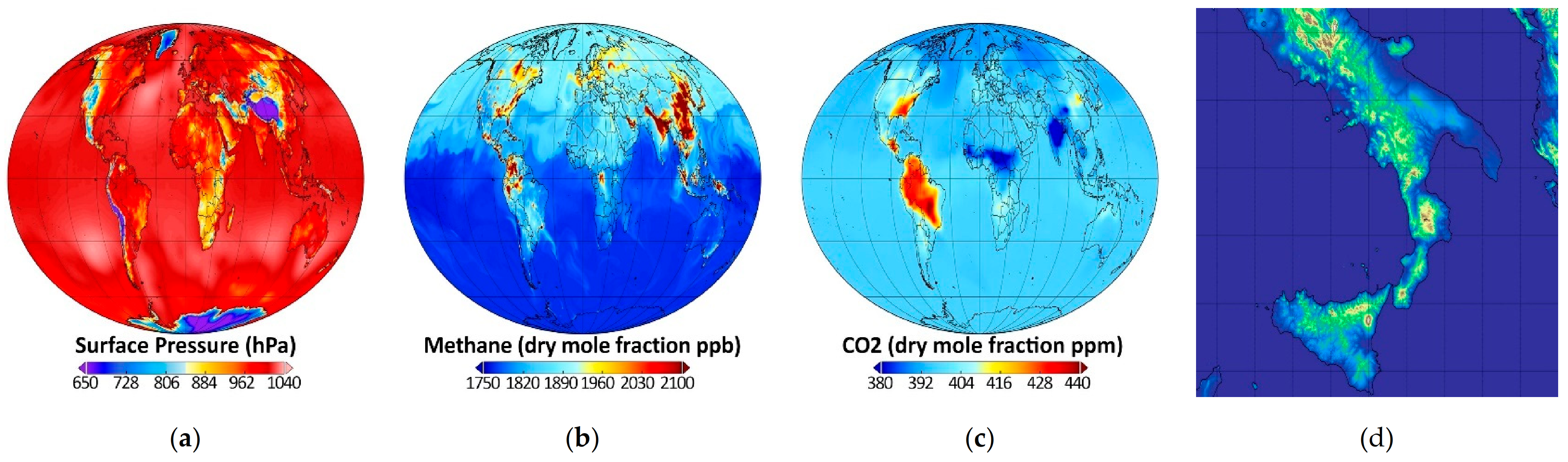
2.1. Ground and Atmosphere Description

The purpose of this section is to define the surface and atmosphere characteristics needed to compute the interactions between light and an Earth target.

2.1.1. Physical and Chemical Properties

Air is considered to be a mixture of ideal gases whose composition is constant for the major components, except for water vapour, although the minor components may vary

$$P=N_{air}RT={\rho }_{air}\frac{R}{M_{air}}T={\rho }_{air}\frac{R}{M_{dry}+q_{H_{2}O}\left(M_{H_{2}O}-M_{dry}\right)}T={\rho }_{air}\frac{R}{M_{dry}}{T}_v$$

(2)

where P is the pressure, N_air is the number of moles of air per unit of volume, R is the ideal gas constant [21], T is the temperature, ρ_air is the air density, M_air/dry/H2O are the molar mass of the moist air, dry air and water vapour, respectively, q_H2O is the specific humidity and T_v is the virtual temperature, which depends on both T and q_H2O.

The molar masses (related to isotopic abundances) are in g/mol [22]: M_air = 28.965, M_H2O = 18.015, M_CO2 = 44.009 and M_CH4 = 16.0425. For any G-gas of molar mass M_G with N_G moles per unit of volume, X_G the mole fraction referring to dry air (expressed in %, ppm or ppb) is associated to the dry mass ratio r_G referring to dry air and to the total mass ratio q_G referring to moist air

$$\begin{array}{c}{X}_G=\frac{N_G}{N_{dry}}=\frac{M_{dry}}{M_G}{r}_G \mathrm{and} q_G=\frac{{\rho }_G}{{\rho }_{air}}=\frac{N_G M_G}{N_{air} M_{air}}=\frac{N_G M_G}{N_{dry} M_{dry}+N_{H_{2}O} M_{H_{2}O}}=\frac{r_G}{1+r_{H_2}}\end{array}$$

(3)

For sensitivity studies, the temperature profile is that of the standard atmosphere [23] defined by the pressure and temperature at sea level, and by the gradients, relative to the geopotential, of the virtual temperature, which are constant in the geopotential bands. The humidity profile decreases exponentially with the geopotential to a minimum value. Analytical functions are used, so no vertical interpolation is required to calculate the different quantities at the various altitudes defined from the arbitrarily fixed ground elevation.

An alternative is to use temperature and humidity values at a set of pressures, taken from the Thermodynamic Initial Guess Retrieval (TIGR) radiosonde database [24] and to perform vertical interpolations at the desired altitudes. As usual, the interpolations used are linear in pressure for humidity and for the virtual temperature deviation from the standard atmosphere, and linear in pressure logarithm for geopotential deviation from the standard atmosphere. Figure 4 shows the temperature and humidity profiles for the standard atmosphere and for five TIGR profiles.

Regarding aerosols and clouds, one of the five vertical aerosol distributions and one of the seven cloud types from the ESA-defined reference model [25] can be selected. XCO₂^ref = 400 ppm and XCH₄^ref = 1780 ppb are the prescribed constant values for the CO₂ and CH₄ profiles. Tests with others values can be performed.

For the orbit simulations, the location of the laser footprints can be determined from the orbital characteristics using the IXION software [26] or taken from any database. Data on meteorological parameters [27], aerosols [28,29] and gas concentrations [30] are taken from operational analyses provided by the European Centre for Medium-Range Weather Forecasts (ECMWF) (Examples of these data sets are shown in Figure 5a–c). Following the habits of the meteorologists, they are interpolated linearly in time and bi-linearly on the horizontal, and then vertically at defined altitudes from the ground elevation. The latter is derived from a Digital Elevation Model (DEM): the EarthEnv DEM [31] at a 90 m resolution (Figure 5d shows this DEM over southern Italy) supplemented by data from the GTOPO30 database [32] at a 1 km resolution for areas where EarthEnv data are missing.

The vertical interpolation consists of first determining the pressure of the target elevation by linear interpolation in geopotential of the logarithm of the pressure, and then interpolating T, q and x_G to this pressure by linear interpolation in pressure. Extrapolations below ground are carried out by keeping a constant gradient from the penultimate layer above ground: zero gradient for specific humidity and any molar mass fraction, and standard gradient for temperature (−6.5 K/km). To preserve boundary layer profiles close to the ground, it is possible to use a more elaborate algorithm, developed at Météo-France (but unpublished), which consists of performing a weighted average between the profile found previously and a profile constructed from the potential temperature of the ground, thus preserving for each layer the gradient of potential temperature on the one hand and relative humidity on the other. A known disadvantage of this approach is the change in the geopotential even at higher altitudes, but this is of little importance here, because the geopotential is only involved in terms of the difference between two levels.

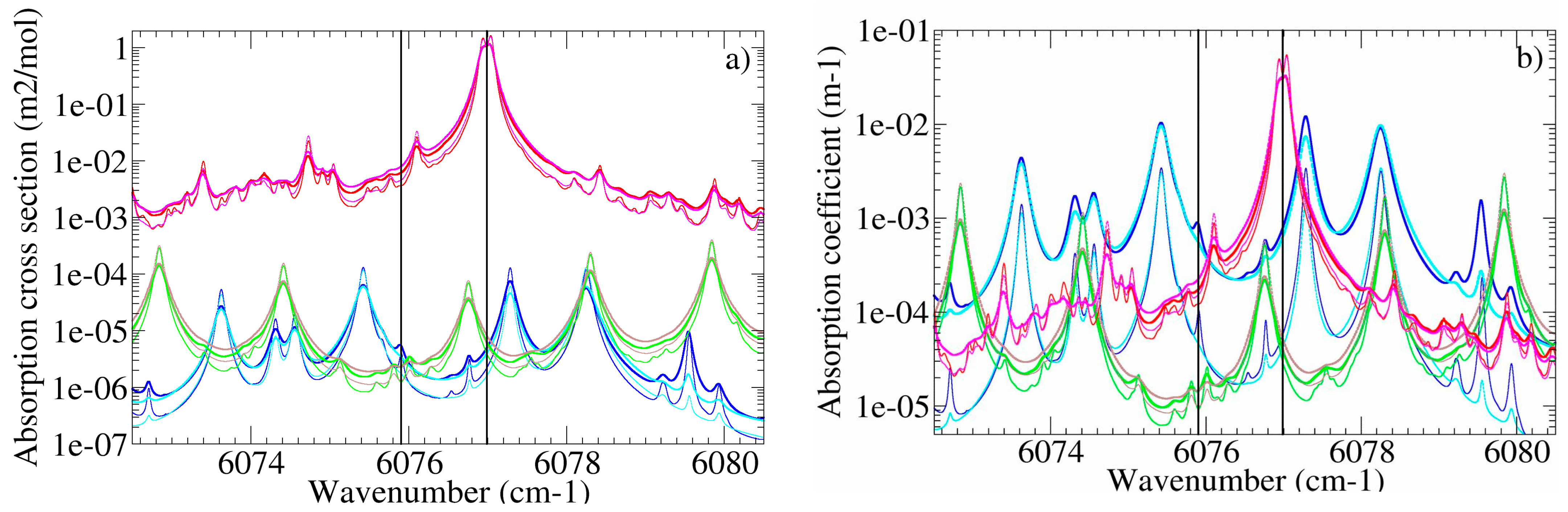
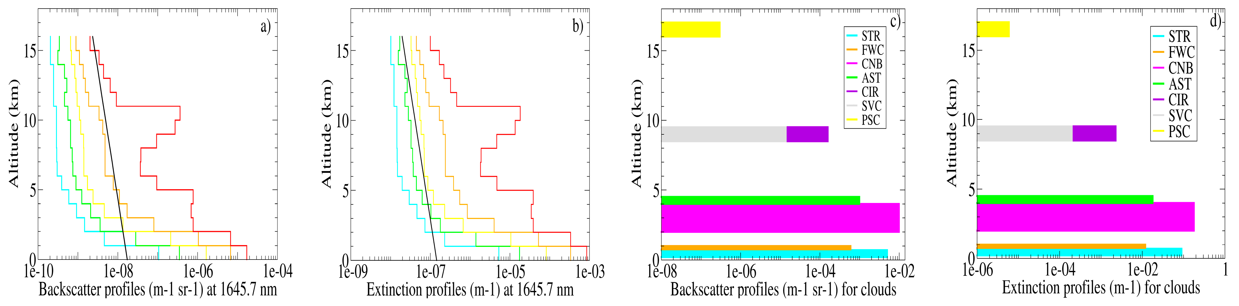
2.1.2. Radiative Properties

The laser emissions of the two MERLIN pulses are nominally centred at λ_On = 1645.5516 nm and λ_Off = 1645.8460 nm. The detection optics contain a filter to limit the incoming solar flux to a Δλ_filter interval of 2 nm. The spectral range is defined in wavelength as [1644.7 nm; 1646.7 nm] or in wavenumber as [6072.75 cm⁻¹; 6080.14 cm⁻¹]. The spectroscopic parameters of the gases of interest (CH₄ but also CO₂ and H₂O) are taken from the GEISA database [33], with recent specific improvements for methane [34,35] and for water vapour [36]. For each G-gas, the vertical distributions of the molar cross sections ${\sigma }_G\left(\nu ,p,T\right)$ are calculated from the thermodynamic description of the atmosphere using the 4A radiative transfer software [37,38] which has been modified to provide absorption cross sections instead of optical thicknesses. The Hartmann–Tran profile [39], recommended by the International Union of Pure and Applied Chemistry, is used for methane lines air-broadening and -shifting and combined with first-order line-mixing approximation. The 4A computations are performed at the maximum spectral resolution of 5 × 10⁻⁴ cm^℡1 (about 15 MHz). Figure 6a shows the absorption cross sections on the spectral region of interest for CH₄, CO₂ and H₂O, and Figure 6b shows the absorption coefficients for typical abundances of these gases.

The atmospheric vertical distributions of extinction and backscatter coefficients for air molecules (α_M and β_M), aerosol particles (α_A and β_A) and cloud droplets (α_C and β_C) are calculated in accordance with the ESA recommendations [25], so that the following relations are imposed

$${\alpha }_M=\frac{8\pi }{3}{\beta }_M, {\alpha }_A=50 {\beta }_A, {\alpha }_{C_{water}}=18 {\beta }_{C_{water}}, {\alpha }_{C_{ice}}=14.3 {\beta }_{C_{ice}}$$

(4)

For molecules, the extinction resulting from scattering is added to the molecular absorption computed above. Figure 7 shows the vertical distribution of backscatter and extinction coefficients estimated at a mean frequency for molecules, aerosols and clouds. It is assumed that these coefficients are not wavelength dependent over a few nanometres.

For clouds, with H_bot and H_top representing the altitudes of the base and top of the cloud layer, respectively, multiple scattering is taken into account for the downwards solar flux. Scattering in the cloud layer is replaced by scattering at the top of the cloud assimilated to a Lambert surface with a hemispherical reflectance R_c. R_c is fixed using τ the optical thickness of the cloud (computed from the extinction coefficient) and g_a = 0.85 the asymmetry factor which characterises the phase function of cloud scattering [41,42]

$$R_C=\frac{\left(1-g_a\right) \tau }{\left(1-g_a\right)\tau + 1} \mathrm{with} \tau ={{\displaystyle \int }}_{H_{bot}}^{H_{top}}{\alpha }_C\left(H\right)dH$$

(5)

The ground is assumed to be a set of scattering surfaces distributed vertically according to $D_{vert}^R\left(H\right)$ with $\int D_{vert}^R\left(H\right)dH=1$. The reflectance of the scattering surfaces varies with incidence and is prescribed as constant for the wavelengths of interest: R_nad for the laser beam (near nadir incidence) and R_hia for sunlight (high incidence angle). For sensibility studies, a typical value of 0.1 is used and $D_{vert}^R\left(H\right)$ is considered as a set of Dirac or Gaussian distributions. For the simulated orbits, the reflectances (see Figure 8) are derived from MODIS [43,44,45] with auxiliary data from SeaWifs and QuikScat for sea reflectances [46] and $D_{vert}^R\left(H\right)$ is estimated, based on the DEM variability between adjacent data, as a weighted sum of nine Dirac distributions.

2.2. From Radiative Properties to Transmission and Backscatter Coefficients

The light transmission factor between the satellite and an atmospheric layer, as well as the scattering coefficient of light towards the satellite from an atmospheric or ground level, are determined according to the observation geometry and the associated Doppler effects. The calculations are performed in spherical geometry with the assumption of horizontal homogeneity, and considering the variation of the speed of light with air density. Multiple scattering is only taken into account for the downward solar flux.

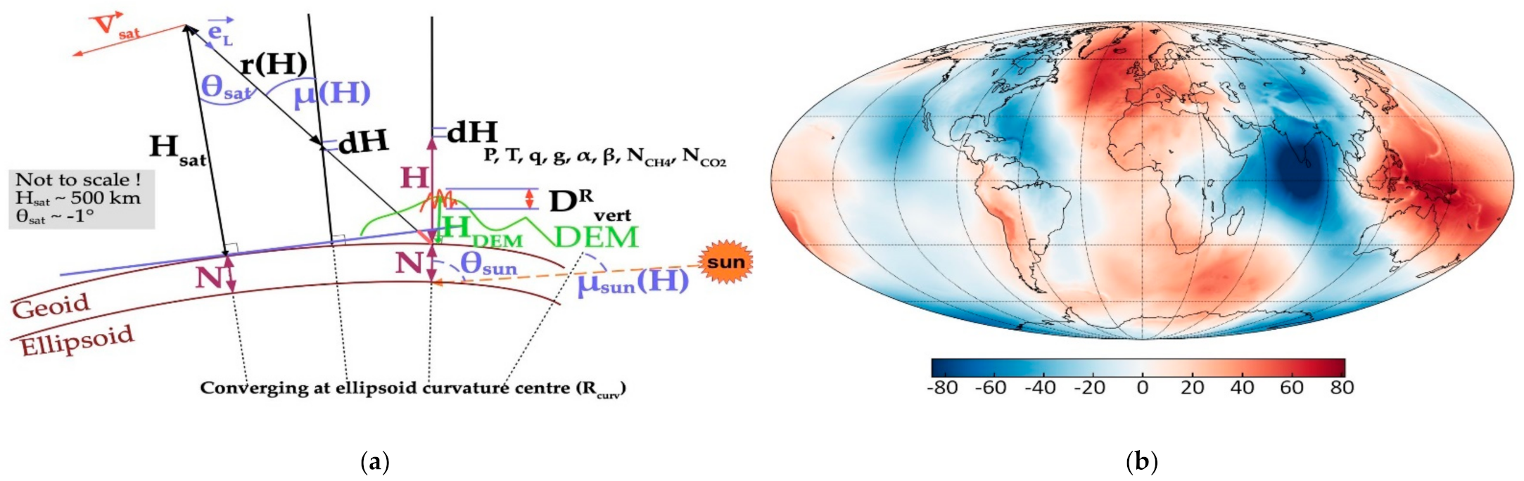
2.2.1. Observation Geometry and Vertical Coordinates

The lidar pulses are emitted in the $\overrightarrow{e_L}$ direction towards the Earth, with an angle θ_sat to the vertical and an angle ${\varphi }_{azimuth}^{laser}$ to the North direction at the satellite location. r indicates the distance between the satellite and the backscatter target along the beam propagation direction. Figure 9a illustrates the observation geometry as modelled with the location of the different variables.

For the geometric calculations, the geodetic system used is WGS84 [47,48]. Its reference ellipsoid (defined by R_Eq = 6378.137 km its terrestrial radius at the equator and e = 0.081819191 its flatness) is locally approximated by a tangent sphere of radius R_curv as a function of latitude lat and azimuth direction ${\varphi }_{azimuth}^{laser}$

$$R_{curv}=\frac{R_{Eq} \left(1-e^2\right)}{\sqrt{\left(1-e^2 si{n}^2\left(lat\right)\right)} \left[1-e^2\left(1-co{s}^2\left(lat\right) co{s}^2\left({\varphi }_{azimuth}^{laser}\right)\right)\right]}$$

(6)

Due to the density inhomogeneities of the Earth, the geoid differs from the reference ellipsoid. H the altitude (relative to the geoid) therefore differs from d_ell the distance to the ellipsoid by N the height of the geoid above the ellipsoid. N is fixed arbitrarily for the sensitivity studies and taken from the Earth Gravitational Model 2008 (EGM08) dataset [49] (shown in Figure 9b) for the orbit simulations

$$H=d_{ell}-N$$

(7)

A spherical atmosphere is used to determine dr, the contribution to the optical path of a vertical layer of thickness dH. With μ(H) the angle at altitude H between the local vertical and the direction of beam propagation, R_curv the local curvature radius of the ellipsoid, N the height of the geoid above the ellipsoid, H_sat = d_sat − N the altitude of the satellite above the geoid and θ_sat = μ(H_sat)

$$\begin{array}{c}dr=\frac{-dH}{cos\left(\mu \left(H\right)\right)} \mathrm{with} \left(R_{curv}+N+H\right) sin\left(\mu \left(H\right)\right)=\left(R_{curv}+N+H_{sat}\right) sin\left({\theta }_{sat}\right)\end{array}$$

(8)

$$\begin{array}{c}\mathrm{and} r\left(H\right)=\left(R_{curv}+N+H_{sat}\right) cos\left({\theta }_{sat}\right)-\left(R_{curv}+N+H\right) cos\left(\mu \left(H\right)\right)\end{array}$$

(9)

The gravity above the geoid is assumed to be the normal gravity above the reference ellipsoid. It varies with latitude and along the vertical. This last dependence is expressed as a Taylor series with altitude. In LIDSIM, the gravity varies as the inverse of H² but the parameter R_grav allows the Taylor series to be adjusted. Then, the gravitational field is defined as

$$g\left(lat,H\right)=g_{Eq} \left(1+g_{1}si{n}^2\left(lat\right)-g_2 si{n}^2\left(2lat\right)\right)\frac{R_{grav}^2}{{\left(R_{grav}+H\right)}^2}$$

(10)

$$\mathrm{and} R_{grav}=\frac{R_{Eq}}{r{g}_1-r{g}_2 si{n}^2\left(lat\right)}$$

(11)

with H the altitude, g_Eq = 9.780327 m/s² the gravity on the geoid at the equator, g₁ = 5.3024 × 10⁻³ and g₂ = 5.8 × 10⁻⁶ two constants to approximate Somigliana’s formula, rg₁ = 1.0068 and rg₂ = 6.7056 × 10⁻³ two other constants to define R_grav, and R_Eq = 6378.137 km the Earth’s radius at the equator.

Figure 10a shows the latitude dependence of the different radii used. As the satellite is intended to be manoeuvred so that $\overrightarrow{e_L}$ forms a constant angle tau = −1° with the direction of the centre of the Earth, θ_sat varies with latitude (see Figure 10b).

To use the meteorological data provided on vertical levels generally defined by their pressure, Z, the geopotential in J/kg, and H, the altitude in m, must be linked

$$dZ=g\left(lat,H\right)dH, Z=g\left(lat,0\right)\frac{H}{1+\frac{H}{R_{grav}}}, H=\frac{Z}{g\left(lat,0\right)-\frac{Z}{R_{grav}}}$$

(12)

The time t_rt required for light to travel the distance r and return is determined using the actual light speed calculated as a function of the air index n_air(H)

$$2dr=\frac{c}{n_{air}\left(H\right)}d{t}_{rt}\left(H\right), t_{rt}\left(H\right)=\frac{2}{c}{{\displaystyle \int }}_{H_{sat}}^H{n}_{air}\left(H\text{'}\right)\frac{-dH\text{'}}{cos\left(\mu \left(H\text{'}\right)\right)}$$

(13)

where c is the light speed in vacuum [21] and n_air(H) is the refractive index along the path. n_air is calculated according to Ciddor [50] from the number of moles per unit volume of dry air and water vapour (N_dry and N_H2O) with two constants cid_dry = 6.49 × 10⁻⁶ and cid_H2O = 5.57 × 10⁻⁶ calculated for a wavelength set to λ_ref = 1645.699 nm and an abundance of CO₂ fixed at XCO₂^ref

$$n_{air}=1+ci{d}_{dry} N_{dry}+ci{d}_{H2O} N_{H2O}$$

(14)

Figure 11 shows the variation of the speed of light with pressure and the corresponding error in the distance to the satellite if the speed of light is assumed constant.

2.2.2. Spectral Distribution of the Lidar Emission and Doppler Effects

In the satellite frame of reference, the lidar emission is assumed to follow a normal frequency distribution with a central frequency ν_o (alternatively ν_On and ν_Off for a pair of pulses) and a standard deviation ${\sigma }_{{\nu }_o}$ corresponding to a full width at half maximum (FWHM) of 60 MHz

$$S_L^{{\nu }_o}\left(\nu \right)=\frac{1}{\sqrt{2\pi } {\sigma }_{{\nu }_o}}{e}^{\frac{-1}{2} \frac{{\left(\nu -{\nu }_o\right)}^2}{{\sigma }_{{\nu }_o}^2}}$$

(15)

Spectral impurities can be introduced by adding similar Gaussian energy distributions on either side of the emission frequency, at significantly lower intensities and at frequencies shifted by one or more free spectral intervals [51].

The movement of the ground or of any air parcels relative to the satellite generates ν_Dop, a Doppler shift between ν_sat the wavelength in the reference frame of the satellite and ν_tar the wavelength in the reference frame of the target. This Doppler shift is proportional to $\overrightarrow{V_{tar}}$ the relative speed

$${\nu }_{tar}=\sqrt{\left(1-\frac{\overrightarrow{V_{tar}}\cdot \overrightarrow{e_L}}{c}\right)/\left(1+\frac{\overrightarrow{V_{tar}}\cdot \overrightarrow{e_L}}{c}\right)}{\nu }_{sat}\approx \left(1-\frac{\overrightarrow{V_{tar}}\cdot \overrightarrow{e_L}}{c}\right){\nu }_{sat}={\nu }_{sat}+{\nu }_{Dop}$$

(16)

where $\overrightarrow{e_L}$ is the unit vector pointing to the laser beam emission direction and c is the speed of light.

As the wind speed’s contribution to the Doppler shift is negligible for near nadir observations (estimated at less than 1 MHz), the generated Doppler shift ν_Dop is constant on the vertical. It is determined by the scalar product $\overrightarrow{V_{sat}}.\overrightarrow{e_L}$ where $\overrightarrow{V_{sat}}$ is the relative speed of the satellite with respect to the ground ($\Vert \overrightarrow{V_{sat}}\Vert$ = 7.6 km/s). Moreover, as the tilt angle tau is chosen to minimise this Doppler effect (tau = −1°), ν_Dop is negligible (less than 5 MHz or 3.3 × 10⁻⁵ cm⁻¹).

In addition, the velocity distribution of the molecules and particles creates a spectral broadening of the light beam scattered by them (illustrated in Figure 12). Assuming a Maxwell–Boltzmann distribution for the velocities of the scatterers (of molar mass M_sca), the probability for velocity V_z on the incident direction is

$$p\left(V_z\right)=\frac{1}{\sqrt{2\pi } {\sigma }_{V_z}}{e}^{\frac{-1}{2} \frac{V_z^2}{{\sigma }_{V_z}^2}} \mathrm{with} {\sigma }_{V_z}=\sqrt{\frac{RT}{M_{sca}}}$$

(17)

The probability distributions of forward and backward frequencies are linked by the conditional probability G_Ray of observing ν_b on the backward path when ν_f is observed on the forward path. Assuming elastic interactions, G_Ray depends only on the shift between ν_b and ν_f which is directly related to V_z and ν_ref, a medium value used for all the frequencies as their dispersion is really small

$$\begin{array}{c}{\nu }_b-{\nu }_f=\frac{-2}{c}{\nu }_{ref}{V}_z\end{array}$$

(18)

$$\begin{array}{c}\mathrm{and} p\left({\nu }_b|{\nu }_f\right)=G_{Ray}\left({\nu }_b-{\nu }_f\right)=\frac{1}{\sqrt{2\pi } {\sigma }_{Ray}}{e}^{\frac{-1}{2} \frac{{\left({\nu }_b-{\nu }_f\right)}^2}{{\sigma }_{Ray}^2}} \mathrm{with} {\sigma }_{Ray}=\frac{2{\nu }_{ref}}{c}\sqrt{\frac{RT}{M_{sca}}}\end{array}$$

(19)

As particles are heavier than molecules, their Brownian motion corresponds to lower individual velocities. Therefore, for the time being, the broadening associated with particles scattering is neglected with respect to the spectral width of the pulse.

Due to the large number of photons in the considered flows, their interactions with molecules or particles are classically treated in a deterministic way.

2.2.3. Vertical Distribution of Transmission and Backscatter Coefficients

T_L(ν,H) refers to the atmospheric transmission at frequency ν, integrated along the direction of the beam propagation between the satellite and the observed scattering target at altitude H. It is calculated from the vertical distribution of the coefficients α_M/A/C(H) representing the extinction due to air molecules, aerosols and clouds, respectively, and from the cross sections σ_G(ν, H) representing the absorption of the minor gases involved

$$\begin{array}{c}\begin{array}{c}{T}_L\left(\nu ,H\right)={\displaystyle {\displaystyle \prod }_{M/A/C}}exp\left(-{{\displaystyle \int }}_H^{H_{toa}}{\alpha }_{M/A/C}\left(H\text{'}\right)\frac{dH\text{'}}{cos\left(\mu \left(H\text{'}\right)\right)}\right)\end{array}{\displaystyle {\displaystyle \prod }_G}exp\left(-{{\displaystyle \int }}_H^{H_{toa}}{N}_G\left(H\text{'}\right) {\sigma }_G\left(\nu ,H\text{'}\right)\frac{dH\text{'}}{cos\left(\mu \left(H\text{'}\right)\right)}\right)\\ =exp\left(-{{\displaystyle \int }}_H^{H_{toa}}\left[{\displaystyle {\displaystyle \sum }_{M/A/C}}{\alpha }_{M/A/C}\left(H\text{'}\right)+{\displaystyle {\displaystyle \sum }_G}{N}_G\left(H\text{'}\right) {\sigma }_G\left(\nu ,H\text{'}\right)\right] \frac{dH\text{'}}{cos\left(\mu \left(H\text{'}\right)\right)}\right)\end{array}$$

(20)

where N_G(H) is the number of moles of G-gas per unit of volume at altitude H and H_toa ≅ 40 km the upper limit of the atmosphere above which light-matter interactions are negligible.

T_L(ν,H) is calculated for the two bands centred on the wavelengths emitted by the lidar and whose width is defined by the Doppler broadening, with a full spectral accuracy of 5 × 10⁻⁴ cm⁻¹ (see Figure 12).

A similar computation, but with a spectral accuracy reduced to 5 × 10⁻² cm⁻¹ to save computing time, is done for T_S(ν,H) the atmospheric transmissions of the solar flux on its own pathway defined by θ_sun the zenith solar angle given at the ellipsoid level

$$T_S\left(\nu ,H\right)=exp\left(-{{\displaystyle \int }}_H^{H_{toa}}\left[{\displaystyle \sum }_{M/A/C}{\alpha }_{M/A/C}\left(H\text{'}\right)+{\displaystyle \sum }_G{N}_G\left(H\text{'}\right) {\sigma }_G\left(\nu ,H\text{'}\right)\right] \frac{dH\text{'}}{cos\left({\mu }_{sun}\left(H\text{'}\right)\right)}\right)$$

(21)

where the angle μ_sun(H) is calculated from the angle θ_sun and the radius $R_{curv}^{sun}$

$$\begin{array}{c}\left(R_{curv}^{sun}+N+H\right) sin\left({\mu }_{sun}\left(H\right)\right)=R_{curv}^{sun} sin\left({\theta }_{sun}\right)\end{array}$$

(22)

$R_{curv}^{sun}$ is determined using Equation (6), from ${\varphi }_{azimuth}^{solar}$, the azimuthal angle of the sun, instead of that of the laser beam.

Furthermore, ${\beta }_l\left({\nu }_b,{\nu }_f,H\right)$ (in m⁻¹ sr⁻¹) the backscatter coefficient for the laser fluxes is given, with ${\delta }_{\nu }$ referring to the Dirac function for the wavenumbers, by

$$\begin{array}{c}{\beta }_l\left({\nu }_b,{\nu }_f,H\right)=\left[R_{nad} D_{vert}^R\left(H\right)+\frac{{\beta }_{A/C}\left(H\right)}{cos\left(\mu \left(H\right)\right)}\right] {\delta }_{\nu }\left({\nu }_b-{\nu }_f\right)+\frac{{\beta }_M\left(H\right)}{cos\left(\mu \left(H\right)\right)} G_{Ray}\left({\nu }_b-{\nu }_f\right)\end{array}$$

(23)

${\beta }_s\left({\nu }_b,{\nu }_f,H\right)$ (in m⁻¹ sr⁻¹) represents the part of the solar flux scattered towards the satellite from the ground or the cloud top and is defined by

$$\begin{array}{c}{\beta }_s\left({\nu }_b,{\nu }_f,H\right)=\left[R_{hia} D_{vert}^R\left(H\right)+\frac{R_c}{\pi } {\delta }_H\left(H-H_{top}\right)\right] {\delta }_{\nu }\left({\nu }_b-{\nu }_f\right)\end{array}$$

(24)

where ${\delta }_H$ refers to the Dirac function for the altitude.

2.3. Radiative Fluxes on the Detector

In this section, the quantities T_L(ν,H), T_S(ν,H), ${\beta }_l\left({\nu }_b,{\nu }_f,H\right)$ and ${\beta }_s\left({\nu }_b,{\nu }_f,H\right)$ determined in the previous section are used together with the instrument properties to specify not only $P_D^L$, the backscattered flux powers, but also $P_D^S$, the solar flux power, at both the On and Off frequencies. Simultaneously, $P_D^M$, the monitoring fluxes powers, are estimated at both the On and Off frequencies.

The main optical properties of the instrument are E_L = 9.5 mJ (alternatively E_On and E_Off for a pair of pulses) the total energy of the emitted laser pulses, E_o(ν) the optical emission efficiency factor, A the effective area of the collecting mirror and D_o(ν) the optical reception efficiency factor including the bandpass filter used to limit the solar flux reaching the detector. This filter is assumed to be an idealised bandpass filter, with a rectangular curve centred on λ_ref =1645.699 nm with Δλ_filter = 2 nm full width. Such a filter does not bias the estimation of DAOD. The effects due to differences in transmissions through the filter for the On and Off pulses are outside the scope of this work but are being studied by Airbus. If necessary, these effects will be integrated into LIDSIM.

2.3.1. From Emitted Lidar Pulses to Backscattered Fluxes on the Detector

The radiative transfer laws provide $F_{/\mathrm{m}}^L\left(H\right)$ (unit m⁻¹) the fraction of energy that returns from altitude H per unit of length after a round trip through the atmosphere

$$F_{/\mathrm{m}}^L\left(H\right)={{\displaystyle \int }}_{{\nu }_b}{D}_o\left({\nu }_b\right) T_L\left({\nu }_b,H\right) \frac{A}{r^2\left(H\right)} {{\displaystyle \int }}_{{\nu }_f}\beta \left({\nu }_b,{\nu }_f+{\nu }_{Dop},H\right) T_L\left({\nu }_f+{\nu }_{Dop},H\right) E_o\left({\nu }_f\right) S_L^{{\nu }_0}\left({\nu }_f\right) d{\nu }_f d{\nu }_b$$

(25)

in the integrals, νf denotes the frequencies for the forward path and νb for the backward path, as seen by the Earth targets.

D_o(ν) and E_o(ν) are assumed to be constant over the range of the transmitted frequencies, and are set to 0.77 and 0.952, respectively. $F_{/\mathrm{m}}^L\left(H\right)$ is then computed using Equation (23)

$$F_{/\mathrm{m}}^L\left(H\right)=D_o E_o \frac{A}{r^2\left(H\right)} \left[\left(R_{nad}{D}_{vert}^R\left(H\right)+\frac{{\beta }_{A,C}\left(H\right)}{cos\left(\mu \left(H\right)\right)}\right) \mathrm{Gat}1\left(H\right)+\frac{{\beta }_M\left(H\right)}{cos\left(\mu \left(H\right)\right)} \mathrm{Gat}2\left(H\right)\right]$$

(26)

where the auxiliary variables Gat1 and Gat2 average the spectral dependencies of the transmissions at the various altitudes

$$\begin{array}{c}\mathrm{Gat}1\left(H\right)={{\displaystyle \int }}_{\nu =-k{\sigma }_{{\nu }_o}}^{k{\sigma }_{{\nu }_o}}{T}_L^2\left({\nu }_0+{\nu }_{Dop}+\nu ,H\right) S_L^{{\nu }_0}\left({\nu }_0+\nu \right) d\nu \end{array}$$

(27)

$$\begin{array}{c}\mathrm{Gat}2\left(H\right)={{\displaystyle \int }}_{\nu \text{'}=-k\left({\sigma }_{{\nu }_o}+{\sigma }_{Ray}\right)}^{k\left({\sigma }_{{\nu }_o}+{\sigma }_{Ray}\right)}{T}_L\left({\nu }_0+{\nu }_{Dop}+\nu \text{'},H\right){{\displaystyle \int }}_{\nu =-k{\sigma }_{{\nu }_o}}^{k{\sigma }_{{\nu }_o}}{G}_{Ray}\left(\nu \text{'}-\nu \right) T_L\left({\nu }_0+{\nu }_{Dop}+\nu ,H\right) S_L^{{\nu }_0}\left({\nu }_0+\nu \right) d\nu d\nu \text{'}\end{array}$$

(28)

with $k=3\sqrt{2}$ the parameter fixing the truncation of the Gaussian distributions.

$P_L^{t_{00}}$, the power emitted by the lidar, is assumed to be distributed in time according to a normal distribution centred on t₀₀ and with standard deviation σ_t corresponding to a full width at half maximum (FWHM) of 20 ns

$$P_L^{t_{00}}\left(t\right)=\frac{E_L}{\sqrt{2\pi } {\sigma }_t}{e}^{\frac{-1}{2} \frac{{\left(t-t_{00}\right)}^2}{{\sigma }_t^2}}$$

(29)

$P_D^L\left(t\right)$ the backscattered laser power reaching the detector at t-time is composed of photons that have done a round trip up to altitude H and were emitted at t − t_rt(H). After a variable change between H and t’ = t_rt(H) − t₀₀, $P_D^L\left(t\right)$ can be expressed as a convolution product over time

$$\begin{array}{c} P_D^L\left(t_{00}+t\right)={{\displaystyle \int }}_H{F}_{/\mathrm{m}}^L\left(H\right) P_L^{t_{00}}\left(t_{00}+t-t_{rt}\left(H\right)\right) dH\\ ={{\displaystyle \int }}_{t\text{'}}{F}_{/\mathrm{s}}^L\left(t_{00}+t\text{'}\right) P_L^{t_{00}}\left(t_{00}+t-\left(t_{00}+t\text{'}\right)\right) dt\text{'}=F_{/\mathrm{s}}^L\otimes P_L^{t_{00}}\left(t_{00}+t\right)\end{array}$$

(30)

$F_{/\mathrm{m}}^L\left(H\right)=F_{/\mathrm{s}}^L\left(t_{rt}\left(H\right)\right)$ is estimated on a set of vertical layers where the radiative properties have been previously computed, but the corresponding set of times t_rt(H) is an irregular basis of time. Therefore, to evaluate the convolution product, $F_{/\mathrm{s}}^L\left(t\right)$ must be resampled. A resampling procedure is implemented to conserve the energy (the number of photons) per time interval. (See Appendix B).

2.3.2. Solar Flux

P_sun(υ) the solar spectrum at the top of the atmosphere (shown in Figure 13) is taken according to Toon [52] and converted in W/m²/cm⁻¹ with Ω_sun = 68.36 μsr the mean solar solid angle.

There is no modelled temporal variation in solar flux on the scale of a pair of pulses, although a displacement of a few metres may induce a significant fluctuation in the presence of clouds. Seasonal and diurnal modulations are only taken into account by ${\theta }_{sun}$ the sun zenith angle. The mean Doppler shift ${\nu }_{Dop}^{sun}$ due to the motion of the Earth on its elliptical orbit and its rotation on itself is less than 0.5 cm⁻¹ and is not taken into account because the seasonal fluctuations of the solar background are out of the scope of this study. As already mentioned, Doppler broadening is also negligible as the solar spectrum does not show any variability at the scale of a few hundredths of cm⁻¹.

$P_D^S$ the solar power on the detector is then constant over time (on a shot scale) and can be obtained as an integral over the scattering altitude

$$P_D^S=D_o \pi {\left(\frac{\delta \theta }{2}\right)}^2 A {{\displaystyle \int }}_0^{H_{toa}}\left(R_{hia}{D}_{vert}^R\left(H\right)+\frac{R_c}{\pi }{D}_{vert}^{R_{cld}}\left(H\right)\right) cos\left({\mu }_{sun}\left(H\right)\right) \mathrm{GatS}\left(H\right) dH$$

(31)

where δθ is the angle determining the field of view (the part of the Earth from which the backscattered photons reach the detector through the receiving optics of the instrument), μ_sun(H) is calculated, using Equation (22) from the angle θ_sun. The auxiliary variable GatS averaging the spectral dependencies of the transmissions is

$$GatS\left(H\right)={{\displaystyle \int }}_{{\nu }_{ref}-\frac{\Delta {\nu }_{filter}}{2}}^{{\nu }_{ref}+\frac{\Delta {\nu }_{filter}}{2}}{T}_L\left({\nu }_{ref}+\nu ,H\right) T_S\left({\nu }_{ref}+\nu ,H\right) P_{sun}\left({\nu }_{ref}-{\nu }_{Dop}^{sun}+\nu \right) d\nu$$

(32)

2.3.3. Energy Monitoring Fluxes

To handle fluctuations in the energy emitted by the laser, the instrument has a calibration unit that records the energy emitted through the same detector and electronic chain as the signal backscattered from the Earth targets [15]. The equation for $P_D^M$, the energy monitoring flux, is simply

$$\begin{array}{c}{P}_D^M\left(t_{00}+t\right)=F_{/\mathrm{s}}^M P_L^{t_{00}}\left(t_{00}+t-t_{d0}\right)\end{array}$$

(33)

where $F_{/\mathrm{s}}^M$ = 0.31 × 10⁻¹² is the fraction of emitted energy injected on the detector by the calibration unit and t_d0 is the delay (calibrated before launch) between the laser emission time and the corresponding detector illumination time. To avoid problems of non-linearity with the detector sensitivity, the energy of the monitoring fluxes must be of the same magnitude as the atmospheric fluxes, so integrating spheres are needed to reduce the energy taken out during the beam emission [18].

2.4. Electronic Chain and Noises

The electronics chain (shown in Figure 14) consists mainly of a detector (APD), a trans-impedance amplifier (TIA) and an analogue-to-digital converter (ADC). The detector is an avalanche photodiode that converts photons into electrons and amplifies their number. The TIA transforms the small current associated with the movement of the electrons into a voltage that can be digitised by the ADC. An anti-aliasing filter (AAF) and other electronics to control the offset (OC) and signal gain (PGA) are located between the TIA and the ADC.

Five fluxes have to be considered on the APD: the On and Off laser beams after their return from the atmosphere, the On and Off laser beams for calibration and the solar flux. Due to the large number of photons, the interactions with the atmosphere and the ground can be considered as deterministic, but in the electronic chain, many stochastic processes have to be taken into account to simulate the mean signals and their variability.

2.4.1. Speckle Effects

A first random process is related to interference on the detector resulting from the differences in optical path between different points in the area illuminated by the laser. Speckle occurs when coherent light is dispersed by wavelength-scale heterogeneities, such as variations in surface roughness or refractive index. The dispersed waves propagate along different optical paths and interfere in any observation plane, showing figures with a granular structure of alternating light and dark spots. Only the energy fluctuations on the detector induced by the speckle of the hard target for the Earth fluxes and by the integrating spheres for the monitoring fluxes are taken into account. The energy variance of each optical flux is a function of M_tav the number of speckle on the collecting mirror [53,54]

$$Var\left(E\right)=\langle {\left(E-\langle E\rangle \right)}^2\rangle =\langle {\left(\mathsf{\Delta }E\right)}^2\rangle =\frac{{\langle E⟩}^2}{M_{tav}}$$

(34)

M_tav the speckle number is determined from S_c the characteristic area, T_c the characteristic time, A = 3850.51 cm² the effective surface of the collecting mirror, δT the time interval considered and P the polarisation index of the flux on the detector

$$M_{tav}=\frac{2}{1+P^2}\left(1+\frac{A}{S_c}\right)\left(1+\frac{\delta T}{T_c}\right)$$

(35)

The laser fluxes are polarised unlike the solar flux. $T_c^{las}$ can be considered infinite for a pulsed laser, because for each pulse there is only one temporal speckle due to the full correlation of the transmitted signal over the pulse duration. Moreover, even if the interference pattern on the detector evolves due to the motion of the satellite relative to the ground, this evolution is negligible over the duration of a laser pulse [54,55]. The speckle noise during a laser pulse is therefore fully correlated.

Table 3. Polarisation index, characteristic area and characteristic time involved in the calculation of M_tav the speckle number for the laser and solar fluxes. λ is the wavelength, div_beam = 181.25 μrad the full divergence of the laser beam at the output of the transmitting telescope measured at the e⁻² energy level, f_rec = 47.04 cm the focal length of the receiving chain, d_APD = 0.2 mm the diameter of the detector and Δλ_filter = 2 nm the filter bandpass.

	P	Sc	Tc	A/Sc	T/Tc	Mtav
Laser flux	1	$\frac{4}{\pi }{\left(\frac{\lambda }{{\mathrm{div}}_{beam}}\right)}^2$ = 105 mm2	∞	3667	0	3668
Solar flux	0	$\frac{4}{\pi }{\left(\frac{\lambda f_{rec}}{d_{APD}}\right)}^2$ = 19 mm2	$\frac{{\lambda }^2}{c\mathsf{\Delta }{\lambda }_{filter}}$ = 4.52 × 10−3 ns	20266	2950	∞

gives the values of the parameters of Equation (35), calculated for the MERLIN instrument characteristics, and $M_{tav}^{las}$ and $M_{tav}^{sun}$ the resulting speckle number for the laser and solar fluxes, respectively. $1/M_{tav}^{sun}$ can be considered as zero due to the large area (field of view of the receiver) from which the solar flux originates and the relatively wide spectral filter.

The monitoring fluxes are depolarised by the integrating spheres, allowing the energy level to be reduced. But the complete analysis of the interference is complex and very dependent on the instrument design (integrating spheres and optical fibres). A value of $M_{tav}^{cal}$ = 1850 is prescribed in LIDSIM following a dedicated study by Airbus. In addition, a specific mechanism is installed to decouple the speckle patterns between each shot [15]. However, decorrelation can only be achieved at the time scale of a shot and not at the time scale of a sample [56]. Thus, the speckle pattern for the monitoring streams is fixed for a full shot but changes from one shot to another. So, the speckle noise on a monitoring pulse is fully correlated.

The effect of speckle noise is to alter the energy estimate of the pulses, each single-shot DAOD can be considered biased. But if there is no correlation on the changes between successive shots, then the final effect on the average energies and an averaged DAOD will be similar to random noise.

2.4.2. Shot Noise

While the speckle noise is due to fluctuations in the optical energy at the detector, arising from interferences reflecting the wave nature of light, the shot noise is due to fluctuations in the number of photons arriving in a given time interval, reflecting the corpuscular nature of light.

The arrival of photons at the detector follows a Poisson law [53]. The mean and variance of the photon number N_ph within any δt-time interval are derived from Mandel’s formula [57], where h is Planck’s constant and υ_On/Off is the frequency

$$\langle N_{ph}\rangle =\frac{\langle E⟩}{h{\nu }_{On/Off}}=\frac{ <P> \delta T}{h{\nu }_{On/Off}}, Var\left(N_{ph}\right)=\frac{\langle E⟩}{h{\nu }_{On/Off}}+\frac{Var\left(E\right)}{{\left(h{\nu }_{On/Off}\right)}^2}$$

(36)

2.4.3. Photoelectric Effect and Avalanche Process in the APD

In the APD, the photoelectric effect is modelled as a Bernoulli dilution characterised by a quantum efficiency η. The avalanche process is characterised by an avalanche factor M = 10 and an excess noise factor F [58]. η and F can be computed from R_det = 0.88 A/W the detector responsivity and κ = 40 the effective ratio of electron and hole ionization coefficients [59]

$$\eta =R_{det}\frac{h\nu }{e} \mathrm{and} F=\kappa M+\left(1-\kappa \right) \left(2-\frac{1}{M}\right)$$

(37)

where h is Planck’s constant [21], e is the charge of an electron [21] and ν is the frequency.

Each photon reaching the detector has the probability p_i of emitting a primary electron with <p_i> = η and Var(p_i) = η (1 − η). Each primary electron is transformed into m_i electrons during the avalanche process with <m_i> = M and Var(m_i) = (F − 1) M². Using Burgess’ variance theorem [60,61] for k independent random variables with the same distribution

$$Var\left({\displaystyle \sum }_{k=1}^N{X}_k\right)={\langle X⟩}^2 Var\left(N\right)+\langle N\rangle Var\left(X\right)$$

(38)

The mean and variance of the number of primary electrons produced by the APD are

$$\begin{array}{c}\langle N_{e_p^{-}}\rangle =\langle {\displaystyle {\displaystyle \sum }_{k=1}^{N_{ph}}}⟩p_i=\eta \langle N_{ph}\rangle \\ Var\left(N_{e_p^{-}}\right)={\eta }^2 Var\left(N_{ph}\right)+\langle N_{ph}\rangle \eta \left(1-\eta \right)=\eta \langle N_{ph}\rangle +{\eta }^2 \left(Var\left(N_{ph}\right)-\langle N_{ph}\rangle \right)\end{array}$$

(39)

and those of the total electron number are

$$\begin{array}{c}\langle N_{e^{-}}\rangle =\langle {\displaystyle {\displaystyle \sum }_{i=1}^{N_{ep}}}{m}_i⟩=M \langle N_{e_p^{-}}\rangle =\eta M \langle N_{ph}\rangle \\ Var\left(N_{e^{-}}\right)=M^2 Var\left(N_{e_p^{-}}\right)+\langle N_{e_p^{-}}\rangle \left(F-1\right)M^2=\eta F{M}^2 \langle N_{ph}\rangle +{\eta }^2{M}^2 \left(Var\left(N_{ph}\right)-\langle N_{ph}\rangle \right)\end{array}$$

(40)

2.4.4. Electronics Noises

Based on the previous paragraph, the APD receives a photon flux P_(t) = δE_(t)/δt of mean power 〈P〉_(t) and generates an electron flux corresponding to the intensity i_p(t) = δq_(t)/δt, with mean 〈i_p〉_(t) and variance Var(i_p)_(t)

$${\begin{array}{c}\langle i_p⟩{}_{\left(t\right)}=\frac{\eta Me}{h{\nu }_{ref}} {\langle P\rangle }_{\left(t\right)}\\ Var{\left(i_p\right)}_{\left(t\right)}=\frac{FMe}{h{\nu }_{ref}} \langle i_p⟩{}_{\left(t\right)} \delta \left(t\right)+{\left(\frac{\eta Me}{h{\nu }_{ref}}\right)}^2 \frac{{\langle P\rangle }_{\left(t\right)}{}^2}{M_{tav}}={\left(\frac{\eta Me}{h{\nu }_{ref}}\right)}^2\left(\frac{F}{\eta }{\langle P\rangle }_{\left(t\right)} h{\nu }_{ref} \delta \left(t\right)+\frac{{\langle P\rangle }_{\left(t\right)}{}^2}{M_{tav}}\right)\end{array}}_{ }$$

(41)

where e is the charge of the electron and δ(t) is the Dirac distribution in time.

The TIA and AAF transform this current into a voltage v₁ but add various electronic noises to the signal. Appendix A defines i_n(t) and uc_n(t) as white noises characterised by î_n and ${\widehat{uc}}_n$ as their Amplitude Spectral Densities (ASD) and amplified by R_i (like the signal) and by R_u, respectively. $\begin{array}{c}{v}_1\left(t\right)=i_p\left(t\right)\otimes R_i+i_n\left(t\right)\otimes R_i+u{c}_n\left(t\right)\otimes R_u\end{array}$, the voltage after the AAF thus has the following mean and variance

$$\begin{array}{c}\langle v_1\rangle \left(t\right)=\langle i_p\rangle \left(t\right)\otimes R_i\\ Var\left(v_1\right)\left(t\right)=Var\left(i_p\right)\left(t\right)\otimes R_i\otimes R_i+\frac{{\widehat{i}}_n{}^2}{2}\Vert R_i^2\Vert +\frac{{\widehat{uc}}_n{}^2}{2}\Vert R_u^2\Vert \end{array}$$

(42)

2.5. From Radiative Fluxes to Digitised Signal

According to the analysis described above, all noises are simulated as Gaussian noises with the appropriate variances and no covariance between samples, except for the speckle noise for which the interference patterns are held constant for a full pulse time by performing a single draw for all discretisation times of that pulse.

Random draws are performed and the electric current time series for the five processed streams are given on a discrete regular time basis {t_j} with t_j+1 − t_j = δt by

$$i_p^{L/M/S}\left(t_j\right)=\frac{\eta Me}{h\nu } \left[P_D^{L/M/S}\left(t_j\right) \left(1+\frac{k_{sp}^{L/M/S}}{\sqrt{M_{tav}^{L/M/S}}}\right)+\sqrt{P_D^{L/M/S}\left(t_j\right) \frac{h\nu }{\delta t}} \left(k_{sn}^{L/M/S}\left(t_j\right)+k_{sB}^{L/M/S}\left(t_j\right) \sqrt{\frac{1}{\eta }-1}+k_{sa}^{L/M/S}\left(t_j\right) \sqrt{\frac{F}{\eta }-\frac{1}{\eta }}\right)\right]$$

(43)

where $k_{sp}^{L/M/S},k_{sn}^{L/M/S}\left(t\right),k_{sB}^{L/M/S}\left(t\right),k_{sa}^{L/M/S}\left(t\right),k_i^{L/M}\left(t\right) \mathrm{and} k_u^{L/M}\left(t\right)$ are random values with standard normal distribution.

The current induced by the solar flux (whose mean does not depend on time) is added to those corresponding to the On/Off signal and those of the monitoring stream to calculate the voltages v₁^L/M

$$v_1{}^{L/M}\left(t_j\right)=\left(i_p^{L/M}\left(t_j\right)+i_p^S\left(t_j\right)+k_i^{L/M}\left(t_j\right) \frac{{\widehat{i}}_n}{\sqrt{2\delta t}}\right)\otimes R_i\left(t_j\right)+k_u^{L/M}\left(t_j\right) \frac{{\widehat{uc}}_n}{\sqrt{2\delta t}}\otimes R_u\left(t_j\right)$$

(44)

The data series are sampled at frequency f_N1 = 75 MHz and an offset xoffset = 13.5 mV is added to ensure that the voltages v₁^L/M have positive values (even with noise). A gain factor calibre = 0.135 is applied before digitisation to nbits = 14 to obtain the digital counts NC^L/M(j) transmitted to the ground, with δ₀ (<1/f_N1) the offset of the transmission time t₀₀ from the left edge of a time interval

$$N{C}^{L/M}\left(j\right)=\frac{\left[v_1^{L/M}\left(t_j\right)+xoffset\right]\ast 2^{nbits}}{calibre} \mathrm{with} t_j=t_{00}-{\delta }_0+\frac{1}{2f_{N1}}+\frac{j}{f_{N1}}$$

(45)

With Equations (30), (31), (33), (43) and (44) and their notations, the digital counts expression is

$$N{C}^{L/M}\left(j\right)=\frac{2^{nbits}}{calibre} [ xoffset+\eta Me \left[F_{/s}^{L/M}\otimes \frac{P_L^{t_{00}}}{h\nu }\otimes R_i\left(t_j\right)+\frac{P_D^S}{h\nu }\otimes R_i\left(t_j\right)\right]+\left[\frac{k_{sp}^{L/M}}{\sqrt{M_{tav}^{L/M}}} \eta Me F_{/s}^{L/M}\otimes \frac{P_L^{t_{00}}}{h\nu }+k_x^{L/M}\left(t_j\right) \left(\sqrt{\frac{F}{\eta }}\frac{\eta Me}{\sqrt{\delta t}} \sqrt{\left(F_{/\mathrm{s}}^{L/M}\otimes \frac{P_L^{t_{00}}}{h\nu }+\frac{P_D^S}{h\nu }\right)}+\frac{{\widehat{i}}_n}{\sqrt{2\delta t}}\right)\right]\otimes R_i\left(t_j\right)+k_u^{L/M}\left(t_j\right) \frac{{\widehat{uc}}_n}{\sqrt{2\delta t}}\otimes R_u\left(t_j\right) ]$$

(46)

The first terms provide the mean value, with the offset and solar terms causing a bias towards the expected mean value. The other terms correspond to random Gaussian noise. To complete the simulation of the MERLIN data, these digital counts are averaged for the times corresponding to high altitude measurements in order to emulate the reduction in the volume of data to be transmitted from the satellite to the ground that will be implemented on board. Figure 15 shows an example of a simulated signal with and without noise.

For further analysis, the following expressions give the mean and covariance of a sum of digital counts over a W-window

$$\langle {\displaystyle \sum }_{t\in W}N{C}^{L/M}\left(t\right)⟩=N_W\frac{2^{nbits}}{calibre} \left(xoffset+\eta Me \frac{P_D^S}{h\nu } \Vert R_i\Vert \right)+\frac{2^{nbits}\eta Me}{calibre} {\displaystyle \sum }_{t\in W}\int F_{/s}^{L/M}\otimes \frac{P_L^{t_{00}}}{h\nu }\left(t\text{'}\right) R_i\left(t-t\text{'}\right) dt\text{'}$$

(47)

$$\begin{gathered} \langle \Delta {\displaystyle \sum }_{t_1\in W}N{C}^{L/M}\Delta {\displaystyle \sum }_{t_2\in W}N{C}^{L/M}⟩={\begin{array}{c}\left(\frac{2^{nbits} \eta Me}{calibre}\right)\end{array}}^2[ \frac{F}{\eta } {\displaystyle \sum }_{t_1\in W \\ {t}_2\in W}\int F_{/s}^{L/M}\otimes \frac{P_L^{t_{00}}}{h\nu }\left(t\right) R_i\left(t_1-t\right) R_i\left(t_2-t\right) dt+\frac{1}{M_{tav}^{L/M}} {\left({\displaystyle \sum }_{t_1\in W}\int F_{/s}^{L/M}\otimes \frac{P_L^{t_{00}}}{h\nu }\left(t\right) R_i\left(t_1-t\right) dt\right)}^2+\frac{F}{\eta } \frac{P_D^S}{h\nu } {\displaystyle \sum }_{t_1\in W \\ {t}_2\in W}\int R_i\left(t_1-t\right) R_i\left(t_2-t\right) dt+\frac{{\widehat{i}}_n{}^2}{2 {\left(\eta Me\right)}^2} {\displaystyle \sum }_{t_1\in W \\ {t}_2\in W}\int R_i\left(t_1-t\right) R_i\left(t_2-t\right) dt+\frac{{\widehat{uc}}_n{}^2}{2 {\left(\eta Me\right)}^2} {\displaystyle \sum }_{t_1\in W \\ {t}_2\in W}\int R_u\left(t_1-t\right) R_u\left(t_2-t\right) dt ] \end{gathered}$$

(48)

3. PROLID: Processing Lidar Data

The processing of the lidar signals follows the MERLIN ATBD [20] but may differ to some extent. PROLID is a research prototype to help define the algorithms that will be used in the official MERLIN ground segment. It is divided into two parts. Firstly, each peak is dated to obtain an estimate of the scattering surface elevation (SSE). The average energy of each peak and its variability are also estimated to derive the differential absorption optical depth (DAOD) along the optical path. Secondly, using ancillary meteorological data, a weighting function, then XCH₄, are computed for each shot. However, due to the noise level, an average over several shots is required to obtain an estimate whose accuracy meets the mission objectives.

3.1. Preliminary Treatments

As the sampling of the signal varies in time with its altitude range, the signal is first reconstructed with a uniform time base by simply assigning the mean value for each corresponding data item.

For each shot, R_out, a region with N_R values without signal influence, is defined and the average signal value on this region is computed

$$P_{out}^{L/M}=\frac{1}{N_R} {\displaystyle \sum }_{R_{out}}N{C}^{L/M}\left(i\right)$$

(49)

$P_{out}^{L/M}$ can be considered as an offset and expressed in terms of the LIDSIM parameters

$$\langle P_{out}^{L/M}\rangle =\frac{2^{nbits}}{calibre} \left(\frac{\eta Me}{h\nu } P_D^S \Vert R_i\Vert +xoffset\right)$$

(50)

When the instrument is in flight, the electronic characteristics, which may drift with time, will be unknown. However, it will be possible, using Equation (51), to estimate U_D the normalised electronic impulse response convolved with the time emission. To avoid broadening due to the vertical distribution of ground reflectance, only data from the energy calibration path will be used. The digital counts of the individual shots used to determine U_D will be averaged after removing the amplitude offset and aligning them to an appropriate time base (the signals will be shifted to fit each peak to its maximum)

$$U_D\left(i\right)=\langle \frac{N{C}^M\left(i\right)-P_{out}^M}{{{\displaystyle \sum }}_{j}N{C}^M\left(j\right)-P_{out}^M}⟩ \approx \frac{P_L^{t00}\otimes R_i\left(i/f_{N1}\right)}{\Vert R_i\Vert f_{N1}} \approx \frac{R_i\left(i/f_{N1}\right)}{\Vert R_i\Vert f_{N1}}$$

(51)

To improve the estimation algorithms that follow, the digital counts are filtered by K_e a function defined such that its convolution with U_D gives G a Gaussian centred function with standard deviation σ_G (σ_G = 6.38 following a recommendation from the ATBD but this value will be adjusted in future work)

$$G\left(i\right)=e^{\frac{-1}{2} \frac{i^2}{{\sigma }_G^2}}=U_D\otimes K_e\left(i\right)$$

(52)

To obtain a smooth K_e function, the low values of G(i) and K_e(i) are forced to zero. After various tests, the limits defining the “low values” are empirically set to a fraction 10⁻⁹ and 10⁻⁶ of the maxima of G and K, respectively. For the processing, $N{C}_F^{L/M}$ and $N{C}_{FC}^{L/M}$ are computed as

$$N{C}_F^{L/M}\left(i\right)=N{C}^{L/M}\left(i\right)\otimes K_e\left(i\right)$$

(53)

$$N{C}_{FC}^{L/M}\left(i\right)=N{C}_F^{L/M}\left(i\right)-P_{R_{out}F}^{L/M} \mathrm{with} P_{R_{out}F}^{L/M}=\frac{1}{N_R}{\displaystyle \sum }_{R_{out}}N{C}_F^{L/M}\left(i\right)$$

(54)

As long as the photon signals on the detector can be considered as quasi-Dirac pulses, the signals received at the ground convolved with K_e have a quasi-Gaussian shape. Despite the different noises, it will then be easier to estimate the time location of the signal, its energy and also its signal-to-noise ratio (SNR).

3.2. Estimations

From the NC_FC(i) digital counts, a peak (or two if there is a transparent cloud) is identified corresponding to the monitoring pulse or return signal record, for each of the two wavelengths On and Off. Each peak corresponds to a photon pulse reaching the detector convolved by the response function. Each peak is associated with the index of its maximum

$$i_{max}^{peak}=\underset{i\in peak}{max}N{C}_{FC}\left(i\right)$$

(55)

To account for the temporal dispersion introduced by the vertical distribution of the target reflectance, the window size used for the estimates is adjusted on the data. The search for the half-value width of the signal is performed on the ν_Off -frequency signal (as it is more energetic). A search interval is set and a first window is constructed by searching, from the limits of the $i_{\max }^{peak}\pm i_{search}$ interval and moving towards the centre, for the first indices $i_{\mathrm{left}}^{peak}$ and $i_{\mathrm{right}}^{peak}$ for which the signal is greater than the half of its maximum $N{C}_{FC}\left(i_{max}^{peak}\right)$. This window is then expanded on either side by half the length of the noise correlation. This procedure is illustrated in Figure 16. The same window size $N_W^{L/M}=i_{\mathrm{right}}^{peakL/M}-i_{\mathrm{left}}^{peakL/M}+1$ is used for the ν_on-frequency signal.

3.2.1. Elevation of the Scattering Target

$i_{peak}^{L/M}$ the recording time of a peak for backscattered or monitoring signals is estimated as centroids on the laser pulse at the ν_Off-frequency

$$i_{peak}^{L/M}=\frac{{{\displaystyle \sum }}_{windowL/M}N{C}_{FC}^{L/M}\left(i\right)i}{{{\displaystyle \sum }}_{windowL/M}N{C}_{FC}^{L/M}\left(i\right)}$$

(56)

The difference between the peak recording times of the Earth and calibration signals is converted into dist, the distance between satellite and target. This is computed by taking into account tdo the delay between a laser emission and its recording (calibrated before launch and arbitrarily fixed at 1760 ns in PROLID for the time being) and with c the average speed of light on the path estimated using H_ref the height scale of the atmosphere

$$\overline{c}=c \left(1-ci{d}_{dry} \frac{P_{00}}{R{T}_{00}} \frac{H_{ref}-H_g}{dist}\right) \mathrm{with} H_{ref}=\frac{R T_{00}}{M_{air} g_{00}}$$

(57)

where P₀₀ = 1013.25 hPa, T₀₀ = 288.15 K, g₀₀ = 9.80665 m s⁻² are the standard values of pressure, temperature and gravity on Earth, R is the ideal gas constant, M_air is the molar mass of dry air and cid_dry = 6.49 × 10⁻⁶ is from Ciddor [50]

$$dist=\frac{c}{2} \left(\frac{i_{peak}^L-i_{peak}^M}{freq{N}_1}+tdo\right)-ci{d}_{dry} \frac{P_{00}}{R{T}_{00}} \left(H_{ref}-H_g\right)$$

(58)

The scattering surface elevation (SSE) is then determined by a geometric computation using a sphere of constant radius R_terre = 6371.226 km instead of the curvature of the geoid (but not a flat Earth, as $SSE=H_{sat}-dist cos{\theta }_{sat}$ would induce a bias of 6 m)

$$\begin{array}{c}SSE=R_{terre}\left(\sqrt{{\left(1+\frac{H_{sat}-dist}{R_{terre}}\right)}^2+2 \frac{dist}{R_{terre}} \left(1+\frac{H_{sat}}{R_{terre}}\right) \left(1-cos{\theta }_{sat}\right)}-1\right)\\ \approx H_{sat}-dist cos{\theta }_{sat}+\frac{{\left(dist sin{\theta }_{sat}\right)}^2}{2R_{terre}}\end{array}$$

(59)

The target is identified as the ground or a cloud by comparing the SSE and the DEM (not yet studied in detail, especially in the case of clouds close to the ground).

3.2.2. Energy Peaks and Their Variability

Proxies $P{P}_{On/Off}^{L/M}$ of the expected values of the peak energy $P_{On/Off}^{L/M}$ are constructed from the digital counts $\left\{N{C}_{FCon/off}^{L/M}\left(i\right)\right\}$ by

$$P{P}_{On/Off}^{L/M}={\displaystyle \sum }_{window}N{C}_{FCOn/Off}^{L/M}\left(i\right)$$

(60)

The digital counts can be divided into a part of photonic origin x_p that is unsteady but results from a convolution by a Gaussian function, and a statistically stationary dark component x_d.

By using the following property of Gaussian distributions

$$\int F\left(t\right) G\left(t_1-t\right) G\left(t_2-t\right)dt=\int F\left(t\right)e^{\frac{-1}{2} \frac{{\left(t_1-t\right)}^2}{{\sigma }_G^2}}{e}^{\frac{-1}{2} \frac{{\left(t_2-t\right)}^2}{{\sigma }_G^2}}dt=e^{\frac{-1}{4} \frac{{\left(t_1-t_2\right)}^2}{{\sigma }_G^2}}\int F\left(t\right)e^{-2 \frac{{\left(\frac{\left(t_1+t_2\right)}{2}-t\right)}^2}{{\sigma }_G^2}}dt$$

(61)

the following relation is established for the photonic part x_p

$$\langle {\left(\Delta x_p\right)}^2⟩={\rm K}\left(x_p\otimes G_{var}\right) \mathrm{and} A_p\left(i\right)=e^{\frac{-1}{4} \frac{i^2}{{\sigma }_G^2}} \mathrm{with} G_{var}\left(i\right)=e^{-2 \frac{i^2}{{\sigma }_G^2}}$$

(62)

A_p is the correlation functions of the photonic part of the signals. A_d is defined as that of the dark component. Then, assuming that the digital counts, which are summed, are contiguous, the following relations are obtained

$${\displaystyle \sum }_{\left(i,j\right)\in E\times E}{A}_{p/d}\left(\left|i-j\right|\right)={\displaystyle \sum }_{i,j=1}^{N_E}{A}_{p/d}\left(\left|i-j\right|\right)=2{\displaystyle \sum }_{u=1}^{N_E-1}\left(N_E-u\right) A_{p/d}\left(u\right)+N_E$$

(63)

Then, with W, the window of size N_W established around the peak in 3.2 and R_out the signal part of size N_R defined in 3.1, the variances of $P{P}_{on/off}^{L/M}$ are estimated, from Equation (48), as

$$Var\left(P{P}_{On/Off}^{L/M}\right)=\frac{{\left(P{P}_{On/Off}^{L/M}\right)}^2}{M_{tav}^{L/M}}+K{\displaystyle \sum }_{\left(i,j\right)\in W\times W}{A}_p\left(\left|i-j\right|\right) \left(N{C}_{On/Off}^{L/M}\left(i\right)-\langle x_d⟩\right)\otimes G_{var}+\langle {\left(\mathsf{\Delta }{x}_d\right)}^2⟩{\displaystyle \sum }_{\left(i,j\right)\in W\times W}{A}_d\left(\left|i-j\right|\right)+{\left(\frac{N_W}{N_R}\right)}^2\left(K{\displaystyle \sum }_{\left(i,j\right)\in R\times R}{A}_p\left(\left|i-j\right|\right) \left(N{C}_{On/Off}^{L/M}\left(i\right)-\langle x_d⟩\right)\otimes G_{var}+\langle {\left(\mathsf{\Delta }{x}_d\right)}^2⟩{\displaystyle \sum }_{\left(i,j\right)\in R\times R}{A}_d\left(\left|i-j\right|\right)\right)$$

(64)

$\langle x_d\rangle$, ${\langle \left(\Delta x_d\right)\rangle }^2$, $\left\{A_d{\left(i\right)}_{i=0,max\left(N_W,N_R\right)-1}\right\}$, $M_{tav}^{L/M}$ and K must be estimated on the ground before launch but they should also be monitored in flight. $\langle x_d\rangle$, ${\langle \left(\mathsf{\Delta }{x}_d\right)\rangle }^2$, $\left\{A_d{\left(i\right)}_{i=0,max\left(N_W,N_R\right)-1}\right\}$ and $M_{tav}^{L/M}$ can be estimated using orbit sections without solar illumination, and K can be estimated [20] using sections with different constant illuminations to establish a regression between the variance of the signal over the section and the average of the G_var-filtered signal over the same section. At present, these quantities are computed in PROLID directly from LIDSIM parameters

$$\begin{array}{c}\langle x_d\rangle =\frac{2^{nbits}}{calibre} xoffset\end{array}$$

(65)

$$\begin{array}{c}\langle {\left(\Delta x_d\right)}^2\rangle ={\left(\frac{2^{nbits}}{calibre}\right)}^2 \left(\frac{{\widehat{i}}_n^2}{2}\Vert {\left(R_i\otimes K_e\right)}^2\Vert +\frac{{\widehat{uc}}_n^2}{2}\Vert {\left(R_u\otimes K_e\right)}^2\Vert \right) \\ ={\left(\frac{2^{nbits}}{calibre}\right)}^2 \Vert R_i\Vert {}^2\sqrt{\pi }{\sigma }_G \left(\frac{{\widehat{i}}_n^2}{2}+\frac{{\widehat{uc}}_n^2}{2}\frac{f_{N1}^2}{2{\sigma }_G^2}\right)\end{array}$$

(66)

$$\begin{array}{c}{A}_d\left(i\right)=\left(1-\frac{1}{1+{\left(\frac{\sqrt{2} {\sigma }_G {\widehat{i}}_n}{f_{N1} {\widehat{uc}}_n}\right)}^2} \left(\frac{i}{\sqrt{2} {\sigma }_G}\right)\right) A_p\left(i\right)\end{array}$$

(67)

$$\begin{array}{c}K=\left(\frac{2^{nbits} \eta Me}{\mathrm{calibre} h\nu }\right) \Vert R_i\Vert \frac{F}{\eta }\end{array}$$

(68)

3.2.3. DAOD along the Optical Path

DAOD_slant on the optical path is estimated from $P{P}_{On/Off}^{L/M}$ the total energy peaks which are assumed to have a Gaussian distribution

$$DAO{D}_{slant}=\frac{-1}{2}ln\left(\frac{P{P}_{On}^{L}P{P}_{Off}^M}{P{P}_{On}^{M}P{P}_{Off}^L}\right)$$

(69)

but for the estimation of its mean, due to the non-linear transformation, a statistical bias coming from the dispersion of the peak energy distribution has to be taken into account [17]

$$<DAO{D}_{slant}>=\frac{-1}{2}ln\left(\frac{<P{P}_{On}^L> <P{P}_{Off}^M>}{<P{P}_{On}^M> <P{P}_{Off}^L>}\right)-\frac{1}{4}\left(\frac{Var\left(P{P}_{On}^L\right)}{<P{P}_{On}^L{>}^2}+\frac{Var\left(P{P}_{Off}^M\right)}{<P{P}_{Off}^M{>}^2}-\frac{Var\left(P{P}_{On}^M\right)}{<P{P}_{On}^M{>}^2}-\frac{Var\left(P{P}_{Off}^L\right)}{<P{P}_{Off}^L{>}^2}\right)$$

(70)

3.3. XCH₄ Retrieval

The actual vertical average of XCH₄, i.e., the XCH₄ column, is

$${\overline{XC{H}_4}}^t:=\frac{\int XC{H}_4\left(h\right) N_{dry}\left(h\right) dh}{\int N_{dry}\left(h\right) dh}=\frac{{{\displaystyle \int }}_0^{P_{DEM}}XC{H}_4\left(p\right) \frac{\left(1-q\left(p\right)\right)}{g\left(p\right) M_{dry}} dp}{{{\displaystyle \int }}_0^{P_{DEM}}\frac{\left(1-q\left(p\right)\right)}{g\left(p\right) M_{dry}} dp}$$

(71)

But, the IPDA method actually averages the observed quantity over the vertical in a specific way. The weighting function WF(p) is used to define a reference observable value corresponding to what the instrument actually observes

$${\overline{XC{H}_4}}^{ref}:=\frac{{{\displaystyle \int }}_0^{P_{DEM}}XC{H}_4\left(p\right) WF\left(p\right) dp}{{{\displaystyle \int }}_0^{P_{DEM}}WF\left(p\right) dp}$$

(72)

The weighting function is estimated using spectroscopic and meteorological auxiliary data

$$\begin{array}{c} WF\left(p\right)=\frac{{\sigma }_{eff}^{C{H}_4}\left({\nu }_{On},p,T_{\left(p\right)}\right)-{\sigma }_{eff}^{C{H}_4}\left({\nu }_{Off},p,T_{\left(p\right)}\right)}{g\left(lat,H\left(p\right)\right) \left(M_{dry}+M_{H_{2}O}{X}_{H_{2}O}\left(p\right)\right)}\\ =\frac{{\sigma }_{eff}^{C{H}_4}\left({\nu }_{On},p,T_{\left(p\right)}\right)-{\sigma }_{eff}^{C{H}_4}\left({\nu }_{Off},p,T_{\left(p\right)}\right)}{g\left(lat,H\left(p\right)\right) M_{dry}} \left(1-q\left(p\right)\right)\end{array}$$

(73)

where g(lat, H(p)) is the vertical acceleration of gravity for latitude lat and altitude H corresponding to pressure p, M_dry is the molar mass of dry air, M_H2O is the molar mass of water vapour, X_H2O is the volume mixing ratio of water vapour to dry air, q is the specific humidity and ${\sigma }_{eff}^{C{H}_4}\left({\nu }_0,p,T\right)$ is the effective absorption cross section of one mole of methane at ν-frequency, p-pressure and T-temperature, which is an average value on the frequencies of the absorption cross sections computed with 4A software

$${\sigma }_{eff}^G\left({\nu }_0,p,T\left(p\right)\right)=\frac{\int \sigma \left(\nu ,p,T\left(p\right)\right) {\tau }_{global}^2\left(\nu ,p\right) S_L^{{\nu }_o+{\nu }_D}\left(\nu \right) d\nu }{\int {\tau }_G^2\left(\nu ,p\right) S_L^{{\nu }_o+{\nu }_D}\left(\nu \right) d\nu }$$

(74)

with ${\tau }_{global}\left(\nu ,p\right)$ calculated from

$$ln\left({\tau }_{global}\left(\nu ,p\right)\right)=-{\displaystyle \sum }_G {{\displaystyle \int }}_0^p\frac{X_G\left(p\text{'}\right) \sigma \left(\nu ,p\text{'},T\left(p\text{'}\right)\right)}{g\left(lat,H\left(p\text{'}\right)\right) M_{dry}} \left(1-q\left(p\text{'}\right)\right) dp\text{'}$$

(75)

Taking into account the residual differences in absorption due to the other gases, PROLID retrieves XCH₄ from the estimation of the mean slant DAOD, with a correction on the optical path length depending on μ, the angle of incidence relative to nadir

$${\overline{XC{H}_4}}^r:=\frac{DAO{D}_{CH4}}{IWF}=\frac{\langle DAO{D}_{slant}⟩ cos\mu -DAO{D}_{H2O}-DAO{D}_{CO2}}{{{\displaystyle \int }}_0^{P_{SSE}}WF\left(p\right) dp}$$

(76)

with IWF the integral of WF, the weighting function, to the SSE pressure, and

$$DAO{D}_G={{\displaystyle \int }}_0^{P_{SSE}}{X}_G\left(p\right) \frac{{\sigma }_{eff}^G\left({\nu }_{On},p,T_{\left(p\right)}\right)-{\sigma }_{eff}^G\left({\nu }_{Off},p,T_{\left(p\right)}\right)}{g\left(lat,H\left(p\right)\right) M_{dry}} \left(1-q\left(p\right)\right) dp$$

(77)

To determine the sources of anthropogenic methane, it is preferable to have an estimate of its concentration averaged over the vertical with greater weight given to the boundary layer. This is why ${\overline{XC{H}_4}}^t$, the actual methane column defined by Equation (71), is not the objective of a mission such as MERLIN, which aims only to find the concentration ${\overline{XC{H}_4}}^{ref}$ defined by Equation (72). Indeed, source identification favours knowledge of a tropospheric column or even a boundary layer column, rather than a complete column, especially since the methane content of the stratosphere is largely decoupled from the sources and governed by its own physics.

3.4. Averaging

Several shots must be averaged to reduce random noise and achieve the mission objectives. Using Equation (70), the expected DAOD over N_shot is obtained by averaging the power ratio of the pulses

$$\overline{DAOD}=\frac{1}{2}ln\left(\frac{{{\displaystyle \sum }}_{k=1}^{N_{shot}}\frac{P{P}_{Off}^L\left(k\right)}{P{P}_{Off}^M\left(k\right)}}{{{\displaystyle \sum }}_{k=1}^{N_{shot}}\frac{P{P}_{On}^L\left(k\right)}{P{P}_{On}^M\left(k\right)}}\right)-0.25\frac{{{\displaystyle \sum }}_{k=1}^{N_{shot}}\frac{Var\left(P{P}_{On}^L\left(k\right)\right)}{P{P}_{On}^M{\left(k\right)}^2}}{{\left({{\displaystyle \sum }}_{k=1}^{N_{shot}}\frac{P{P}_{On}^L\left(k\right)}{P{P}_{On}^M\left(k\right)}\right)}^2}+0.25\frac{{{\displaystyle \sum }}_{k=1}^{N_{shot}}\frac{Var\left(P{P}_{Off}^L\left(k\right)\right)}{P{P}_{Off}^M{\left(k\right)}^2}}{{\left({{\displaystyle \sum }}_{k=1}^{N_{shot}}\frac{P{P}_{Off}^L\left(k\right)}{P{P}_{Off}^M\left(k\right)}\right)}^2}$$

(78)

according to Tellier et al. [17], a weighting factor is defined that gives more weight to shots with more signal

$$w\left(k\right)=\frac{\frac{P{P}_{Off}^L\left(k\right)}{P{P}_{Off}^M\left(k\right)}}{{{\displaystyle \sum }}_{l=1}^{N_{shot}}\frac{P{P}_{Off}^L\left(l\right)}{P{P}_{Off}^M\left(l\right)}}$$

(79)

Then, ${\overline{XC{H}_4}}^a$, the methane column averaged over N_shot, is obtained as follows

$${\overline{XC{H}_4}}^a=\frac{\overline{DAOD}cos\left({{\displaystyle \sum }}_{k=1}^{N_{shot}}w\left(k\right) \mu \left(k\right)\right)-{{\displaystyle \sum }}_{k=1}^{N_{shot}}w\left(k\right) DAO{D}_{H2O/CO2}\left(k\right)}{{{\displaystyle \sum }}_{k=1}^{N_{shot}}w\left(k\right) IWF\left(k\right)}$$

(80)

A correction must be made for the variability of geophysical conditions for the different pairs of pulses during the averaging interval. This is an iterative correction formula, but only one iteration is required [17]

$${\overline{XC{H}_4}}^b=2{\overline{XC{H}_4}}^a+0.5\frac{log\left({{\displaystyle \sum }}_{k=1}^{N_{shot}}w\left(k\right)e^{-2{\overline{XC{H}_4}}^{a}IWF\left(k\right)}\right)}{{{\displaystyle \sum }}_{k=1}^{N_{shot}}w\left(k\right)IWF\left(k\right)}$$

(81)

4. Results and Discussion

4.1. Order of Magnitude of Some Characteristic Values

Table 4. Estimated value for the detector quantum efficiency, the detector noise factor, the speckle number both for the Earth signal and the calibration path, the response function norm, the offset value and the standard deviation of the electronic noise (in digital counts or in mV), and the K parameter defined by Equations (62) and (68).

η	F	${\mathit{M}}_{\mathit{t}\mathit{a}\mathit{v}}^{\mathit{l}\mathit{a}\mathit{s}}$	${\mathit{M}}_{\mathit{t}\mathit{a}\mathit{v}}^{\mathit{c}\mathit{a}\mathit{l}}$	$\mathit{\Vert }{\mathit{R}}_{\mathit{i}}\mathit{\Vert }$	$\mathit{\langle }{\mathit{x}}_{\mathit{d}}\mathit{\rangle }$	$\sqrt{\mathit{\langle }{\left(\mathsf{\Delta }{\mathit{x}}_{\mathit{d}}\right)}^2\mathit{⟩}} \mathit{\ast }$	K
0.715	7.18	2882	1850	998,798 Ω	1638.4 or 13.5 mV	383.5 or 3.16 mV	9.98 × 10−7

* the standard deviation of the electronic noise is the sum of one component coming from the current noise and another coming from the voltage noise.

gives the order of magnitude obtained from the above equations for several important instrumental parameters of the MERLIN mission using the LIDSIM and PROLID software.

In summary, a photon incident on the detector gives a mean current over a 13.3 ns sampling interval of 0.086 nA which becomes, in steady state, a potential difference at the output of the detection chain of 85.8968 μV and finally a digital count of 10.425.

For a numerical simulation with a standard atmosphere, no aerosol and no clouds, and a standard deviation for the dispersion of the scattering ground levels of 15 m, the transmissions are 0.984 for the Off laser pulse, 0.297 for the On laser pulse and 0.853 for the sunlight in the spectral filter. The DAOD is then 0.61319. The window size for estimating the pulse energy is 35 samples for the monitoring pulse and is expanded to 43 samples for the ground signal due to the vertical distribution of the scattering surface.

Table 5. For two ground reflectance values: the number of photons in the laser pulses (calibration, Off and On), the number per samples of photons in the solar flux and their contribution in mV to both the signal offset and the additional variability (for a sun zenith angle of 70° and 80°), the electronic noise (both for the amplified part as signal or current noise and for the differently amplified part or voltage noise) expressed in photons per sample and by its contribution in mV to the bias and dispersion, and finally, the 3 SNRs of the laser peak energy: calibration, Off and On (with and without solar flux).

	Ref = 0.1	Ref = 0.01
Ncal	18 786 photons	id
NOff	8 539 photons	865 photons
NOn	2 608 photons	268 photons
Nsun(70°)	56.41 photons or 4.85 mV ± 1.73 mV	5.641 photons or 0.485 mV ± 0.55 mV
Nsun(80°)	27.21 photons or 2.34 mV ± 1.20 mV	2.721 photons or 0.234 mV ± 0.38 mV
Nnoise	187.30 ph + 0.91 ph or ± 3.16 mV ± 0.22 mV	id
SNRcal	29.5 without sun 29.1 with the sun at 70°	id
SNROff	20.4 without sun 19.5 with the sun at 70°	2.75 without sun smaller but nearly the same with the sun at 70°
SNROn	7.8 without sun 7.4 with the sun at 70°	0.86 without sun smaller but nearly the same with the sun at 70°

gives the total number of photons per pulse reaching the detector, the number of sunlight photons per 13.3 ns time interval, the equivalent number of photons for the noise in the same interval (187.3 associated with ${\widehat{i}}_n$, the overall electrical intensity noise and 0.9 associated with ${\widehat{uc}}_n$ the voltage noise, both defined in Appendix A) and the SNR for the different recorded pulses. In the absence of any other noise, a shot-level SNR of 4.2 is required to achieve 2% accuracy on methane retrieval for a set of 140 shots.

4.2. Signal Validation

Numerous experiments were carried out without noise, to verify the developed software, by varying technical parameters such as: the vertical resolution and upper limit in altitude for radiative computations, vertical and spectral resolutions for transmission calculations, the temporal resolution for electronic simulations and ground reflectance representation. In all noise-free cases, the SSE (defined by Equation (59)) is retrieved to better than 0.1 m and XCH₄ is retrieved to better than 0.5 ppb. Sensitivity experiments were also conducted for methane content, ground elevation, weather patterns, aerosol amounts and cloud types.

Figure 17 shows the impact of methane content, atmosphere type and aerosol content on the digitised signal. These experiments use as a reference point a standard atmosphere without aerosol with a methane content of 1780 ppb. For the methane sensitivity: the methane content varies from 1760 to 1800 ppb; for the atmosphere type sensitivity: the typical atmospheres from the TIGR database are used, with the temperature and humidity profiles given in Figure 4; for the aerosol sensitivity: the five distributions recommended by ESA [25] are used (see Figure 7). To quantify the sensitivity of the digital counts to methane concentration, it can be noted that there was an increase of 40 ppb of methane results in a decrease of 23 counts out of 2788 for the peak of the On signal (no change for the Off signal), i.e., only about 2 photons less per sample. When changing the type of atmosphere, even for times with no laser signal, the signal level varies by about the same amount of 20 counts. This is mainly due to the average humidity of the atmosphere which, as it increases, decreases the solar radiation and the laser radiation for the Off beam, which is placed on a water line (see Figure 6). The variation for the On beam is different—humidity variations are dominated by variations in the temperature profile. Indeed, at the methane multiplet where the On wavelength is located, the absorption increases when the temperature decreases (see Figure 6b). The signal is more perturbed by the type of atmosphere than by a change of 40 ppb of methane, highlighting the importance of good temperature and humidity profiles for recovering methane columns. The aerosols, for their part, can significantly attenuate the signal to a level that will not exceed that of noise when taken into account. In addition, it should be noted that at ground level, the aerosols contribute to the bias in the determination of the SSE. This is because photons backscattered from aerosols close to the ground mix with those returned from the ground itself and distort the return pulse. This effect will be investigated in a future study on the accuracy of SSE determination.

For all cloud types, except polar stratospheric clouds and sub-visible cirrus clouds, the laser signal is fully scattered, so there is no echo from the ground (see Figure 18). But in the absence of noise, it is still possible to retrieve XCH₄ content above the cloud layer with similar precision and accuracy as over cloudless ground. Note the importance of the change in the background signal with sunlight.

Figure 19 shows the weighting functions computed from Equation (73) for representative atmospheres from the tropics to the poles. They are mainly determined by the choice of the On and Off wavelengths. As desired, these functions are not too sensitive to the air mass and are practically uniform over a large part of the atmosphere. They decay in the stratosphere, which means that MERLIN only observes a tropospheric methane column. The maximum sensitivity is around 700 hPa. A maximum in the boundary layer would have been preferred, but it is not physically possible. Finally, for the error budget, it should be noted that the use of the vertical resolution of the ECMWF model in PROLID results in a quadrature error in the estimation of these weight functions, leading to a bias of about 0.2 ppb in the methane retrieval.

4.3. Noise Impact

Simulations were performed one hundred times for the standard atmosphere [23] with 140 random realisations of the noise each time. Figure 20 shows the shot-by-shot distribution of the DAOD retrieved in PROLID minus the actual DAOD computed in LIDSIM, as well as the distribution of XCH₄ retrieved minus the actual value of 1780 ppb. As expected, with a bias of 21 ppb and a standard deviation of 303 ppb, the shot-by-shot XCH₄ is not usable. Therefore, averaging several shots is necessary. Moreover, it should be noted that the distribution is not Gaussian, which implies that the averaging has to be performed with care, as explained above in Section 3.4, in line with what is studied in Tellier et al. [17].

Figure 21 shows the distribution of XCH₄ averaged over 140 shots before and after subtracting the statistical bias on the DAOD. Before subtracting, the average XCH₄ distribution has a bias of 30 ppb and a standard deviation of 27 ppb. After subtracting the statistical bias, estimated from the SNRs estimates (see. Equation (78)), the experimental bias is reduced to 1 ppb and the standard deviation becomes 26 ppb.

4.4. Full Orbit Simulations

CNES provided the orbital data (sun-synchronous orbits at 6.00 UTC) and ECMWF the atmospheric data for 18 June 2019. The orbit starts north of Canada, descends over the Pacific, passes over Antarctica, ascends over Africa, Tunisia, Sardinia, Corsica and the Alps, before ending over Greenland. Figure 22 shows the ground track and the DEM interpolated on it. Complete orbits of 810 cells of 140 shots were simulated, without aerosols or clouds, first without any noise and then with the instrumental noise. Some experiments were also performed with vertically uniform XCH₄, but the results presented here correspond to experiments with realistic methane profiles.

Figure 23 shows the actual ground reflectivity used along the ground track. At high latitudes, the reflectivity data show some anomalies. At the same latitudes, due to the nature of the ground (snow or ice), the reflectivity is close to zero according to the reflectivity data set used. There is therefore no signal. The corresponding points are eliminated in the processing.

Figure 24 shows along the ground track: in green, the full column average of XCH₄ computed (Equation (71)) as the ratio of the number of moles of methane to the number of moles of air; in red, the XCH₄ reference computed (Equation (72)) as the vertical average concentration obtained by applying the MERLIN weighting function; in black, the XCH₄ retrieved shot-by-shot provided by PROLID (Equation (81)). As mentioned earlier, the objective of the MERLIN mission is to retrieve the XCH₄ reference, not the full column average of XCH₄. Without noise, the retrievals are almost perfect. For this reason, the red curve is hidden by the black dots in Figure 24a. This is neither the object of the Merlin mission nor of this article, but one can observe the differences and their geographical variability between the full column of methane (green curve) and the reference methane that MERLIN will be able to observe (red curve hidden by the black points). For the simulation that was carried out, the differences are positive in the Northern Hemisphere and negative in the Southern Hemisphere, with the major differences being over the relief. Figure 24b shows the highly noisy nature of the shot-by-shot inversion (note that the green and red curves are the same on Figure 24a,b).

Table 6. For the experiments with and without instrumental noise, per shots and per 50 km cell, the differences between retrieved SSE and XCH₄ and their references in terms of mean bias and mean standard deviation calculated over the number of points for which XCH₄ can be retrieved (points with sufficient signal due to sufficient reflectivity).

	SSE (in m)			XCH4 (in ppb)
Experiment	Per Shot		Per Cell	Per Shot		Per Cell
	without Noise	with Noise	with Noise	without Noise	with Noise	with Noise
Number of points	113,400	96,385 (85%)	669 (83%)	113,400	96,239 (85%)	669 (83%)
Bias	0.02	0.	0.	0.07	11.3	1.2
Standard deviation	0.03	1.7	0.1	0.10	250.3	16.0

summarises the results on SSE and methane content, shot-by-shot and also averaged over 140 shots (7 s). There are less data for the experiment with instrumental noise than for the one without, because, for points with low reflectivity, the signal is lost in the noise, and it is then impossible to process these points. The determination of the SSE requires only the Off pulse, whereas the XCH₄ also requires the On pulse. Therefore, the number of shots considered for the SSE and for the XCH₄ is not the same. For the 7 s averages, only those for which all 140 shots are available are considered. This will be improved later on.

The standard deviation of 16 ppb for these 7 s average data is better than the 26 ppb presented in the previous section for the tests with a standard atmosphere, just because here the reflectivities used (see Figure 23) are on average higher than the value of 0.1 taken in the tests of the previous section. It should be noted that this standard deviation clearly depends on the number of shots available for averaging, and will therefore increase when aerosols and clouds are considered.

For the experiments with instrumental noise, Figure 25 shows, for each 50 km cell, the differences between the retrieved SSE and XCH₄ and their references. In the experiments without noise, a slight modulation of errors was observed as a function of the ground altitude and the temperature profile. However, the experiments with instrumental noise give homogeneous results in quality over the whole orbit, except of course for a strong dependence on the target reflectivity. This is consistent with the MERLIN random noise budgets, established by Airbus and CNES, which show that the instrumental noise is predominant [2].

Various sources of error are not taken into account in this study, such as non-linearities of the laser emission or detection, or the lack of knowledge of certain parameters: in particular, the emitted wavelengths, the satellite attitude or the state of the atmosphere. The main source of error not taken into account is that induced by uncertainties in operational meteorological analyses. Nevertheless, preliminary studies (not detailed here) have indicated that it is less than 0.9 pp. Thus, although there is no geophysical noise in these simulations (the weighting function is computed with the actual values used to simulate the MERLIN data in LIDSIM), the present study can conclude on the performance achieved by the MERLIN mission. Figure 26 shows the performance of the modelled instrument compared to that expected by the users.

The target performance does not seem to be achievable as the speckle noise alone gives a standard deviation of 60 ppb for one shot and 5 ppb for a 50 km average [54]. However, breakthrough performance is reached and optimisation of the processing parameters can further improve it.

5. Conclusions

The LIDSIM and PROLID software packages have been developed and tested, respectively, to generate MERLIN lidar signals and to produce XCH₄ data from them. They are proving to be powerful tools for preparing satellite missions such as MERLIN. They have been developed with enough generality to be applicable to other IPDA lidar missions and many parts of these packages can be useful for preparing other types of satellite missions or even for simulating ground-based remote sensing instruments. In this line of work, PROLID has already been used on CHARM-F data [19] provided by the DLR.

In the framework of MERLIN, numerous sensitivity tests have been performed on both technical parameters and geophysical conditions. Orbital simulations investigating the impact of the clouds and aerosols remain to be carried out, as well as the updating of the detection chain in order to follow the choices of the instrument manufacturer (Airbus). In the future, the level of performance estimated by our tools will be systematically compared with that estimated by the performance model used by Airbus and CNES to validate the design of the MERLIN instrument. LIDSIM and PROLID will also be used to optimise the pre-processing of digital counts and to study the possibility of retrieving cloud and canopy heights from MERLIN data (secondary products).

The simulations carried out so far and presented in this paper confirm that the current MERLIN design, as simulated here, achieves the ambitious breakthrough performance set for the mission.

References

1. Ehret, G.; Bousquet, P.; Pierangelo, C.; Alpers, M.; Millet, B.; Abshire, J.B.; Bovensmann, H.; Burrows, J.P.; Chevallier, F.; Ciais, P.; et al. MERLIN: A French-German Space Lidar Mission Dedicated to Atmospheric Methane. Remote Sens. 2017, 9, 1052. [Google Scholar] [CrossRef] [Green Version]
2. Bousquet, P.; Pierangelo, C.; Bacour, C.; Marshall, J.; Peylin, P.; Ayar, P.V.; Ehret, G.; Bréon, F.M.; Chevallier, F.; Crevoisier, C.; et al. Error Budget of the MEthane Remote LIdar missioN and Its Impact on the Uncertainties of the Global Methane Budget. JGR Atmos. 2018, 123, 766–785. [Google Scholar] [CrossRef]
3. Crevoisier, C.; Clerbaux, C.; Guidard, V.; Phulpin, T.; Armante, R.; Barret, B.; Camy-Peyret, C.; Chaboureau, J.P.; Coheur, P.F.; Crpeau, L.; et al. Towards IASI-new generation (IASI-NG): Impact of improved spectral resolution and radiometric noise on the retrieval of thermodynamic, chemistry and climate variables. Atmos. Meas. Tech. 2014, 7, 4367–4385. [Google Scholar] [CrossRef] [Green Version]
4. Irizar, J.; Melf, M.; Bartsch, P.; Koehler, J.; Weiss, S.; Greinacher, R.; Erdmann, M.; Kirschner, V.; Perez Albinana, A.; Martin, D. Sentinel-5/UVNS. In Proceedings of the International Conference on Space Optics—ICSO 2018, Chania, Greece, 12 July 2019; Volume 11180, p. 1118004. [Google Scholar] [CrossRef] [Green Version]
5. Cressot, C.; Chevallier, F.; Bousquet, P.; Crevoisier, C.; Dlugokencky, E.J.; Fortems-Cheiney, A.; Frankenberg, C.; Parker, R.; Pison, I.; Scheepmaker, R.A.; et al. On the consistency between global and regional methane emissions inferred from SCIAMACHY, TANSO-FTS, IASI and surface measurements. Atmos. Chem. Phys. 2014, 14, 577–592. [Google Scholar] [CrossRef] [Green Version]
6. GAW Report n°213. In Proceedings of the 17th WMO/IAEA Meeting on Carbon Dioxide, Other Greenhouse Gases and Related Tracers Measurement Techniques (GGMT-2013), Beijing, China, 10–13 June 2013; World Meteorological Organization: Geneva, Switzerland, 2014.
7. Ehret, G.; Kiemle, C.; Wirth, M.; Amediek, A.; Fix, A.; Houweling, S. Space-borne remote sensing of CO2, CH4, and N2O by integrated path differential absorption Lidar: A sensitivity analysis. Appl. Phys. B Lasers Opt. 2008, 90, 593–608. [Google Scholar] [CrossRef] [Green Version]
8. Frankenberg, C.; Aben, I.; Bergamaschi, P.; Dlugokencky, E.J.; Van Hees, R.; Houweling, S.; Van der Meer, P.; Snel, R.; Tol, P. Global column-averaged methane mixing ratios from 2003 to 2009 as derived from SCHIAMACHY:Trends and variability. J. Geophys. Res. Atmos. 2011, 116, D04302. [Google Scholar] [CrossRef]
9. Butz, A.; Guerlet, S.; Hasekamp, O.; Schepers, D.; Galli, A.; Aben, I.; Frankenberg, C.; Hartmann, J.M.; Tran, H.; Kuze, A.; et al. Toward accurate CO2 and CH4 observations from GOSAT. Geophys. Res. Lett. 2011, 38, L14812. [Google Scholar] [CrossRef] [Green Version]
10. Morino, I.; Uchino, O.; Inoue, M.; Yoshida, Y.; Yokota, T.; Wennberg, P.O.; Toon, G.C.; Wunch, D.; Roehl, C.M.; Notholt, J.; et al. Preliminary validation of column-averaged volume mixing ratios of carbon dioxide and methane retrieved from GOSATshort-wavelength infrared spectra. Atmos. Meas. Tech. 2011, 4, 1061–1076. [Google Scholar] [CrossRef] [Green Version]
11. Crevoisier, C.; Nobileau, D.; Fiore, A.M.; Armante, R.; Chedin, A.; Scott, N.A. Tropospheric methane in the tropics—First year from IASI hyperspectral infrared observations. Atmos. Chem. Phys. 2009, 9, 6337–6350. [Google Scholar] [CrossRef] [Green Version]
12. Hu, H.; Landgraf, J.; Detmers, R.; Borsdorff, T.; Aan de Brugh, J.; Aben, I.; Butz, A.; Hasekamp, O. Toward Global Mapping of Methane with TROPOMI: First Results and Intersatellite Comparison to GOSAT. Geophys. Res. Lett. 2018, 45, 3682–3689. [Google Scholar] [CrossRef]
13. Glumb, R.; Davis, G.; Lietzke, C. The TANSO-FTS-2 instrument for the GOSAT-2 greenhouse gas monitoring mission. In Proceedings of the 2014 IEEE International Geoscience and Remote Sensing Symposium (IGARSS), Quebec City, QC, Canada, 6 November 2014; pp. 1238–1240. [Google Scholar] [CrossRef]
14. Kiemle, C.; Quatrevalet, M.; Ehret, G.; Amediek, A.; Fix, A.; Wirth, M. Sensitivity studies for a space-based methane lidar mission. Atmos. Meas. Tech. 2011, 4, 2195–2211. [Google Scholar] [CrossRef] [Green Version]
15. Nikolov, S.; Wührer, C.; Kühl, C.; Bode, M.; Hupfer, W.; Lucarelli, S. MERLIN: Design of an IPDA LIDAR instrument. CEAS Space J. 2019, 11, 437–457. [Google Scholar] [CrossRef]
16. Amediek, A.; Fix, A.; Wirth, M.; Ehret, G. Development of an OPO system at 1.57 μm for integrated path DIAL measurement of atmospheric carbon dioxide. Appl. Phys. 2008, 92, 295. [Google Scholar] [CrossRef] [Green Version]
17. Tellier, Y.; Pierangelo, C.; Wirth, M.; Gibert, F.; Marnas, F. Averaging bias correction for the future space-borne methane IPDA lidar mission MERLIN. Atmos. Meas. Tech. 2018, 11, 5865–5884. [Google Scholar] [CrossRef] [Green Version]
18. Fix, A.; Quatrevalet, M.; Amediek, A.; Wirth, M. Energy calibration of integrated path differential absorption lidars. Appl. Opt. 2018, 57, 7501–7514. [Google Scholar] [CrossRef]
19. Amediek, A.; Ehret, G.; Fix, A.; Wirth, M.; Büdenbender, C.; Quatrevalet, M.; Kiemle, C.; Gerbig, C. CHARM-F a new airborne integrated-path differential-absorption lidar for carbon dioxide and methane observations: Measurement performance and quantification of strong point source emissions. Appl. Opt. 2017, 56, 5182–5197. [Google Scholar] [CrossRef] [PubMed]
20. Wirth, M. MERLIN ATBD: Algorithm Theoretical Basis Document Part 1/Top Level Algorithms for Primary L1/2 Products: MLN-PLDP-ATBD-90001-PI, Version 1, Revision 2; CNES: Toulouse, France, 2018.
21. Newell, D.; Tiesinga, E. The International System of Units (SI), 2019 Edition, Special Publication (NIST SP), National Institute of Standards and Technology, Gaithersburg, MD, USA. Available online: https://doi.org/10.6028/NIST.SP.330-2019 (accessed on 1 July 2021).
22. Haynes, W.M. (Ed.) Handbook of Chemistry and Physics, 97th ed.; CRC Press: Boca Raton, FL, USA, 2017; p. 2643. ISBN 978-1498754293. [Google Scholar]
23. COESA (Committee on Extension to the Standard Atmosphere). U.S. Standard Atmosphere, 1976; U.S. Government Printing Office: Washington, DC, USA, 1976. Available online: https://www.ngdc.noaa.gov/stp/space-weather/online-publications/miscellaneous/us-standard-atmosphere-1976/us-standard-atmosphere_st76-1562_noaa.pdf (accessed on 1 July 2021).
24. Chevallier, F.; Chédin, A.; Chéruy, F.; Morcrette, J.-J. TIGR-like atmospheric-profile databases for accurate radiative-flux computation. Q. J. R. Meteorol. 2000, 126, 777–785. [Google Scholar] [CrossRef]
25. Reference Model of the Atmosphere. Internal Report, ESA, EOP-PI/2006-12-19 Issue 02. 2006. Available online: https://earth.esa.int/eogateway/documents/20142/37627/Aeolus-L1B-Algorithm-ATBD.pdf (accessed on 1 July 2021).
26. Capderou, M. Handbook of Satellite Orbits; Springer: Cham, Switzerland, 2014. [Google Scholar] [CrossRef]
27. Dee, D.P.; Uppala, S.M.; Simmons, A.J.; Berrisford, P.; Poli, P.; Kobayashi, S.; Andrae, U.; Balmaseda, M.A.; Balsamo, G.; Bauer, P.; et al. The ERA-Interim reanalysis: Configuration and performance of the data assimilation system. Q. J. R. Meteorol. Soc. 2011, 137, 553–597. [Google Scholar] [CrossRef]
28. Morcrette, J.J.; Boucher, O.; Jones, L.; Salmond, D.; Bechtold, P.; Beljaars, A.; Benedetti, A.; Bonet, A.; Kaiser, J.W.; Razinger, M.; et al. Aerosol analysis and forecast in the ECMWF Integrated Forecast System. Part I: Forward modelling. J. Geophys. Res. 2009, 114, D06206. [Google Scholar] [CrossRef]
29. Benedetti, A.; Morcrette, J.J.; Boucher, O.; Dethof, A.; Engelen, R.J.; Fisher, M.; Flentje, H.; Huneeus, N.; Jones, L.; Kaiser, W.; et al. Aerosol analysis and forecast in the ECMWF Integrated Forecast System. Part II: Data assimilation. J. Geophys. Res. 2009, 114, D13205. [Google Scholar] [CrossRef] [Green Version]
30. Agusti-Panareda, A.; Diamantakis, M.; Bayona, V.; Klappenbach, F.; Butz, A. Improving the inter-hemispheric gradient of total column atmospheric CO2 and CH4 in simulations with the ECMWF semi-Lagrangian atmospheric global model. Geosci. Model Dev. 2017, 10, 1–18. [Google Scholar] [CrossRef] [Green Version]
31. Robinson, N.; Regetz, J.; Guralnick, R.P. EarthEnv-DEM90: A nearly-global, void-free, multi-scale smoothed, 90m digital elevation model from fused ASTER and SRTM data. ISPRS J. Photogramm. Remote Sens. 2014, 87, 57–67. [Google Scholar] [CrossRef]
32. Danielson, J.J.; Gesch, D.B. Global Multi-Resolution Terrain Elevation Data 2010 (GMTED2010); US Department of the Interior; US Geological Survey Open File Report, 2011. Available online: http://pubs.usgs.gov/of/2011/1073/pdf/of2011-1073.pdf (accessed on 1 July 2021).
33. Jacquinet-Husson, N.; Armante, R.; Scott, N.A.; Chedin, A.; Crépeau, L.; Boutammine, C.; Bouhdaoui, A.; Crevoisier, C.; Capelle, V.; Boonne, C.; et al. The 2015 edition of the GEISA spectroscopic database. J. Mol. Spectrosc. 2016, 327, 31–72. [Google Scholar] [CrossRef] [Green Version]
34. Delahaye, T.; Maxwell, S.E.; Reed, Z.D.; Lin, H.; Hodges, J.T.; Sung, K.; Devi, V.; Warneke, T.; Tran, H. Precise methane absorption measurements in the 1.64 μm spectral region for the MERLIN mission. JGR Atmos. 2016, 121, 7360–7370. [Google Scholar] [CrossRef]
35. Delahaye, T.; Ghysels, M.; Hodges, J.T.; Sung, K.; Armante, R.; Tran, H. Measurement and modeling of air-broadened methane absorption in the MERLIN spectral region at low temperatures. JGR Atmos. 2019, 124, 3556–3564. [Google Scholar] [CrossRef]
36. Vasilchenko, S.; Tran, H.; Mondelain, D.; Kassi, S.; Campargue, A. Accurate absorption spectroscopy of water vapour near 1.64 µm in support of the MEthane Remote LIdar missioN (MERLIN). J. Quant. Spectrosc. Radiat. Transf. 2019, 235, 332–342. [Google Scholar] [CrossRef]
37. Scott, N.A.; Chédin, A. A fast line-by-line method for atmospheric absorption computations: The Automatized Atmospheric Absorption Atlas. J. Appl. Meteor. 1981, 20, 802–812. [Google Scholar] [CrossRef] [Green Version]
38. Chéruy, F.; Scott, N.A.; Armante, R.; Tournier, B.; Chedin, A. Contribution to the development of radiative transfer models for high spectral resolution observations in the infrared. J. Quant. Spectrosc. Radiat. Transf. 1995, 53, 597–611. [Google Scholar] [CrossRef]
39. Ngo, N.H.; Lisak, D.; Tran, H.; Hartmann, J.-M. An isolated line-shape model to go beyond the Voigt profile in spectroscopic databases and radiative transfer codes. J. Quant. Spectrosc. Radiat. Transf. 2013, 129, 89–100. [Google Scholar] [CrossRef]
40. Vaughan, J.M.; Brown, D.W.; Nash, C.; Alejandro, S.B.; Koenig, G.G. Atlantic atmospheric aerosol studies: 2. Compendium of airborne backscatter measurements at 10.6μm. JGR Atmos. 1995, 100, 1043–1065. [Google Scholar] [CrossRef]
41. Meador, W.E.; Weaver, W.R. Two-stream approximations to radiative transfer in planetary atmospheres: A unified description of existing methods and a new improvement. J. Atmos. Sci. 1980, 37, 630–643. [Google Scholar] [CrossRef] [Green Version]
42. Peng, Y.; Lohmann, U.; Leaitch, R.; Banic, C.; Couture, M. The cloud albedo-cloud droplet effective radius relationship for clean and polluted clouds from RACE and FIRE.ACE. JGR Atmos. 2002, 107, AAC 1-1–AAC 1-6. [Google Scholar] [CrossRef]
43. Vermote, E.F.; Roger, J.C.; Ray, J.P. MODIS Surface Reflectance User’s Guide (Collection 6, Version 1.4). May 2015. Available online: https://modis-land.gsfc.nasa.gov/pdf/MOD09_UserGuide_v1.4.pdf (accessed on 1 July 2021).
44. Bréon, F.-M.; Maignan, F.; Leroy, M.; Grant, I. Analysis of hopt spot directional signatures measured from space. JGR Atmos. 2002, 107, AAC 1-1–AAC 1-15. [Google Scholar] [CrossRef]
45. Maignan, F.; Bréon, F.-M.; Lacaze, R. Bidirectional reflectance of Earth targets: Evaluation of analytical models using a large set of spaceborne measurements with emphasis on the hot spot. Remote Sens. Environ. 2004, 90, 210–220. [Google Scholar] [CrossRef]
46. Noveltis Consortium. A Surface Reflectance DAtabase for ESA’s Earth Observation Missions (ADAM) Technical Note 4 for ESA Study Contract Nr C4000102979, NOV-3895-NT-12121. 2013. Available online: https://nebula.esa.int/sites/default/files/neb_study/1089/C4000102979ExS.pdf (accessed on 1 July 2021).
47. Imagery, National and Agency, Mapping Department of Defense. World Geodetic System 1984: Its Definition and Relationships with Local Geodetic Systems. (TR8350.2); National Imagery and Mapping Agency: St. Louis, MO, USA, 2000.
48. Moritz, H. Geodetic Reference System 1980. J. Geod. 2000, 74, 128–162. [Google Scholar] [CrossRef]
49. Pavlis, N.K.; Holmes, S.A.; Kenyon, S.C.; Factor, J.K. The development and evaluation of the Earth Gravitational Model 2008 (EGM2008). J. Geophys. Res. 2012, 117, B04406. [Google Scholar] [CrossRef] [Green Version]
50. Ciddor, P.E. Refractive index of air: New equations for the visible and near infrared. Appl. Optics. 1996, 35, 1566–1573. [Google Scholar] [CrossRef] [PubMed]
51. Mahnke, P.; Klingenberg, H.H.; Fix, A.; Wirth, M. Dependency of injection seeding and spectral purity of a single resonant KTP optical parametric oscillator on the phase matching condition. Appl. Phys. 2007, 89, 1–7. [Google Scholar] [CrossRef] [Green Version]
52. Toon, G.C. Solar Line List for GGG2014, TCCON Data Archive; The Carbon Dioxide Information Analysis Center, Oak Ridge National Laboratory: Oak Ridge, TN, USA, 2014. [CrossRef]
53. Goodman, J.W. Statistical Optics; John Wiley & Sons: Hoboken, NJ, USA, 1985. [Google Scholar]
54. Cassé, V.; Gibert, F.; Edouart, D.; Chomette, O.; Crevoisier, C. Optical Energy Variability Induced by Speckle: The Cases of MERLIN and CHARM-F IPDA Lidar. Atmosphere 2019, 10, 540. [Google Scholar] [CrossRef] [Green Version]
55. Ohtsubo, J.; Asakura, T. Velocity measurement of a diffuse object by using time-varying speckles. Opt. Quant. Electron. 1976, 8, 523–529. [Google Scholar] [CrossRef]
56. Liu, Z.; Hunt, W.; Vaughan, M.; Hostetler, C.; McGill, M.; Powell, K.; Winker, D.; Hu, Y. Estimating random errors due to shot noise in backscatter lidar observations. Appl. Opt. 2006, 45, 4437–4447. [Google Scholar] [CrossRef] [PubMed]
57. Mandel, L. Fluctuations of Photon Beams: The Distribution of the Photo-Electrons. Proc. Phys. Soc. 1959, 74, 233–243. [Google Scholar] [CrossRef]
58. Teich, M.C.; Saleh, B.E.A. Effects of random deletion and additive noise on bunched and antibunched photon-counting statistics. Opt. Lett. 1982, 7, 365–367. [Google Scholar] [CrossRef]
59. Mc Intyre, R.J. Distribution of gains in uniformly multiplying avalanche photodiodes: Theory. IEEE Trans. Electron Devices 1972, 19, 703–713. [Google Scholar] [CrossRef]
60. Burgess, R.E. Homophase and heterophase fluctuations in semiconducting crystals. Discuss. Faraday Soc. 1959, 28, 151–158. [Google Scholar] [CrossRef]
61. Van Vliet, K.M.; Rucker, L.M. Noise associated with reduction, multiplication and branching processes. Phys. Stat. Mech. Appl. 1979, 95, 117–140. [Google Scholar] [CrossRef]
Figure 1. (a) Principle of the satellite-based IPDA lidar technique applied to MERLIN; (b) Optical flow diagram for MERLIN (for the meaning of the variables see the text).
Remotesensing 13 02679 g001
Figure 2. User requirements for the MERLIN mission translated in terms of standard deviation for different averaging times (the red/blue/green curves correspond to the threshold/breakdown/target cases respectively). The vertical black line indicates the performance required for one shot. The lines are continuous from 7 s, the expected averaging time for MRLIN data.
Remotesensing 13 02679 g002
Figure 3. Flowcharts: (a) LIDSIM and (b) PROLID. In yellow the inputs, in blue the processes, in green some variables, in red those related to noise, in grey the impulse responses of the electronic chain, and in purple the outputs.
Remotesensing 13 02679 g003
Figure 4. (a) Temperature profiles and (b) humidity profiles for standard atmosphere (in black) and for five typical TIGR atmospheres (tropical in red, mid-latitude in green and dark green, polar in cyan and blue).
Remotesensing 13 02679 g004
Figure 5. Global maps of: (a) surface pressure, (b) total methane column, (c) total carbon dioxide column from ECMWF available on the 21 September 2014 12H UTC and (d) EarthEnv DEM over southern Italy.
Remotesensing 13 02679 g005
Figure 6. (a) The molar absorption cross sections (m2/mol) and (b) the molar absorption coefficient (m−1) from 6072.5 cm−1 to 6080.5 cm−1 for methane/water vapour/carbon dioxide (respectively in red-magenta/blue-cyan/green-brown) and for four sets of pressure and temperature. The molar absorption coefficients are calculated with a concentration of 1780 ppb for CH4, 1% at P = 1013.25 hPa and 1‰ at P = 500 hPa for H2O and 400 ppm for CO2.The curves are bold red/blue/green for P = 1013.25 hPa and T = 300 K, bold magenta/cyan/brown for P = 1013.25 hPa and T = 250 K, thin red/blue/green for P = 500 hPa and T = 280 K and thin magenta/cyan/brown for P = 500 hPa and T = 220 K. The vertical black lines indicate the spectral position of the Off and On laser emissions.
Remotesensing 13 02679 g006
Figure 7. (a) Backscatter and (b) extinction profiles at 1645.7 nm prescribed from the ESA atmospheric reference model [25] for molecules (black curve) and aerosols (each curve comes from a climatological database of Atlantic aerosols [40]: lower decile value (LD) in blue, lower quartile (LQ) in green, median in yellow, upper quartile (HQ) in orange and upper decile (HD) in red). (c) Backscatter and (d) extinction profiles prescribed by the ESA atmospheric reference model [25] in the NIR-Visible region for different type of clouds: stratus, fair weather cumulus, cumulonimbus, altostratus, cirrus, sub-visible cirrus and polar stratospheric clouds.
Remotesensing 13 02679 g007
Figure 8. Global maps of zenith reflectance around 1.6 μm on a monthly basis (here June). (a) for a nadir incidence (hot spot configuration), the map provided by the company Estellus under a CNES contract, over the continents with a lat/lon resolution of 1/120°. These data are used for the laser fluxes even though, with an incidence angle of −1°, there is no specular reflectivity in the MERLIN context. (b) for a solar incidence angle of 65°, the map provided by the company Noveltis under an ESA contract [46], with resolution of 1/10°. These data are used for sunlight even if the incidence angle (given the choice of orbit) is larger as the database has too many artefacts at higher angles of incidence.
Remotesensing 13 02679 g008
Figure 9. (a) Observation geometry (for the notations see the text). (b) Global map of geoid height provided by EGM08 (in meter).
Remotesensing 13 02679 g009
Figure 10. (a) Latitude dependences of Rellipsoid the ellipsoid radius (distance to the Earth centre), of Rcurv the tangent sphere radius (for two azimuths) and of Rgrav the radius used for gravity computation. (b) For one orbit: in black tau the fixed tilt of the platform in geodetic frame, in blue θsat = μ(Hsat) the angle between the beam direction and the vertical at the satellite level and in red μ(0) the satellite viewing angle from the ellipsoid.
Remotesensing 13 02679 g010
Figure 11. For the pressure levels in hPa of a standard atmosphere: (a) the speed of light in km/s; (b) the distance offset in m if the speed of light is assumed to be the same as in the vacuum.
Remotesensing 13 02679 g011
Figure 12. For (a) the Off and (b) the On beam, the dependence of the logarithm of the energy on the wavenumber: emitted (blue), after Doppler broadening by molecules at 300 K (green) or by particles (assumed 32 times heavier than molecules) at 300 K (red). The dots are at the spectral resolution of the 4A computations (5 × 10⁻⁴ cm−1).
Remotesensing 13 02679 g012
Figure 13. Solar spectrum over the width of the MERLIN spectral filter. The red (resp. blue) line indicates the wavelength of the laser beam On (resp. Off).
Remotesensing 13 02679 g013
Figure 14. Electronic chain diagram from photon detector to digitised data.
Remotesensing 13 02679 g014
Figure 15. Example of signals. (a) without noise. (b) with noise. The On (blue) and Off (red) signals correspond to the same digitisation index because the sampling index of each is counted from its own emission time. The vertical distribution of the ground reflectance is symmetrical with respect to its mean value. The asymmetry of the signals over time is only due to the shape of the response function (see Appendix A).
Remotesensing 13 02679 g015
Figure 16. Summary of the process of determining the averaging window on the νOff-frequency signal.
Remotesensing 13 02679 g016
Figure 17. Sensitivity of the Off and On laser pulse records to (a) the methane content, (b) the TIGR atmosphere used [24], (c) the aerosol content (see Figure 6, MS: molecular scattering only). For the reference experiment, the maximum value is 4762 for the Off signal and 2788 for the On signal.
Remotesensing 13 02679 g017
Figure 18. Position and strength of cloud and ground signals for various cloud types (see Figure 7) for a solar zenith angle (SZA). (a) SZA = 90°. (b) SZA = 70°. The rightmost peak around 20,200 is the ground echo.
Remotesensing 13 02679 g018
Figure 19. For 5 typical TIGR atmospheres. (a) The weighting functions. (b) The differences in methane absorption cross sections between λOn and λOff.
Remotesensing 13 02679 g019
Figure 20. Histograms over 14,000 shots of the deviations from the actual values. (a) for the DAOD (with a sampling of 3.5 × 10⁻⁴ unitless). (b) for the XCH4 (with a sampling of 1 ppb).
Remotesensing 13 02679 g020
Figure 21. Histograms over 100 averages (over 140 shots) of the deviations from the true value for XCH4 (with a sampling of 1 ppb). In blue before subtraction of the statistical bias, and in green after.
Remotesensing 13 02679 g021
Figure 22. (a) Ground track for the orbit used. (b) DEM at the MERLIN targets along this track.
Remotesensing 13 02679 g022
Figure 23. Ground reflectivity from the database used. (a) for laser beams (incidence angle close to 0). (b): for solar flux (huge incidence angle).
Remotesensing 13 02679 g023
Figure 24. For a complete orbit, the actual (or full column average) XCH4 in green, theXCH4 reference in red and the retrieved XCH4 in black. (a) experiment without noise. (The curve in red for the XCH4 reference is not visible because everywhere the retrieved methane is very close to its reference value); (b) with instrumental noise.
Remotesensing 13 02679 g024
Figure 25. Averaged over 7 s (about 50 km), the black curve gives the average and the blue area shows the one standard deviation variability of the results shot-by-shot. (a). Differences between the SSE retrieved by PROLIDL1 and the horizontal average over 140 shots of the DEM. (b). XCH4 retrieved by PROLIDL2, the actual XCH4 and the reference XCH4 (green and red curve as in Figure 24) also averaged over 140 shots.
Remotesensing 13 02679 g025
Figure 26. MERLIN performances estimated with LIDSIM and PROLID (the red/blue/green curves correspond to the threshold/breakthrough/target performances, respectively). The cyan dots represent the tests described in Section 4.3 (at the shot and cell level before and after removing the statistical bias), and the orange diamonds represent the results obtained in this section (for one shot and for one cell).
Remotesensing 13 02679 g026