Article

Prototype Calibration with Feature Generation for Few-Shot Remote Sensing Image Scene Classification

1
School of Electronics and Information, Northwestern Polytechnical University, Xi’an 710072, China
2
Honors College, Northwestern Polytechnical University, Xi’an 710072, China
3
Perelman School of Medicine, University of Pennsylvania, Philadelphia, PA 19104, USA
*
Author to whom correspondence should be addressed.
These authors contributed equally to this work.
Remote Sens. 2021, 13(14), 2728; https://doi.org/10.3390/rs13142728
Submission received: 19 June 2021 / Revised: 7 July 2021 / Accepted: 9 July 2021 / Published: 12 July 2021

Abstract

:
Few-shot classification of remote sensing images has attracted attention due to its important applications in various fields. The major challenge in few-shot remote sensing image scene classification is that limited labeled samples can be utilized for training. This may lead to the deviation of prototype feature expression, and thus the classification performance will be impacted. To solve these issues, a prototype calibration with a feature-generating model is proposed for few-shot remote sensing image scene classification. In the proposed framework, a feature encoder with self-attention is developed to reduce the influence of irrelevant information. Then, the feature-generating module is utilized to expand the support set of the testing set based on prototypes of the training set, and prototype calibration is proposed to optimize features of support images that can enhance the representativeness of each category features. Experiments on NWPU-RESISC45 and WHU-RS19 datasets demonstrate that the proposed method can yield superior classification accuracies for few-shot remote sensing image scene classification.

Graphical Abstract

1. Introduction

Remote sensing images captured by satellites contain rich information of land-cover targets, which have been widely applied in kinds of scenarios such as road detection [1], ecological monitoring [2], disaster prediction, and other fields [3,4]. Scene classification of remote sensing images aims to classify novel images into corresponding categories based on the captured information [5,6], which has become an important research direction at present. Few-shot scene classification prefers to classify images into corresponding categories with limited samples [7], which is of great importance since limited labeled samples can be acquired in various applications. Few-shot classification of remote sensing images has great application prospects in environmental monitoring, biological protection, resource development and so on, which can greatly reduce the requirements of field research and manual annotation.
Deep learning has achieved admirable performance in traditional image classification [8,9], which generally need a large number of labeled data for training. Deep neural networks perform well with complex network structure and sufficient prior knowledge [10,11]. However, if the labeled training set is inadequate, there would be obvious overfitting of the deep model and deviation of feature expression. As for various remote sensing applications, it is hard to acquire labeled samples, and collecting annotated data is quite time-consuming [12]. In addition, the training process of deep neural network consumes a lot of computing resources, which needs to be re-trained if some hyper-parameters are not set properly.
Inspired by the procedure of humans connecting unknown things with prior knowledge, few-shot learning has been developed for tasks of limited supervised information, which has the ability to recognize novel categories using only a few annotated samples [7]. Few-shot learning methods can be roughly divided into three categories: meta learning, metric learning [13], and transfer learning [14]. Meta learning is also known as learning to learn [15], which performs the role of guiding the learning of new tasks. As for metric learning methods, the similarity of two images is compared to estimate whether they are belonging to the same category, in which the higher the similarity, the greater the possibility of belonging to the same category. Different metric learning methods have been proposed [16], where various distance measures are utilized for few-shot classification. Transfer learning is proposed to apply prior knowledge from relevant tasks towards novel tasks on the premise of pre-trained models.
The above-mentioned methods pay attention to training a well-performed classifier or a robust learning model for few-shot learning, which ignores the significance of feature expression. As for scene classification of remote sensing images, the classifier may not perform well when the learned features cannot effectively represent the corresponding category [17]. Furthermore, in the tasks of few-shot remote sensing image scene classification, high similarity of images between categories, and great differences in images within the same category are great issues [18]. Some examples can be found from Figure 1. It is observed from Figure 1a that these images reflect intra-class consistency, which are well-suited to few-shot classification. In Figure 1b, images belonging to the beach category have different colors, and images in the palace category show different textures, which reflects the phenomenon of large intraclass variances. In Figure 1c, it is obvious that images of freeway and railway have similar texture features, and images of lake and golf course have almost consistent backgrounds, which indicates that there are high similarities between categories. Moreover, there may be diverse objects in a remote sensing images, which also influences the performance of scene classification. These issues seriously affect the classification performance, and effective feature representation for remote sensing images should be considered.
Considering the characteristics and large scales of remote sensing images, some deep networks [19] have been utilized to extract features in order to obtain more semantic information in the early research, such as VGG16, AlexNet, and so on. However, it is hard to train the deep networks with insufficient annotated samples, especially in few-shot situation. Most recent proposed methods pay more attention to enhance features. In DLA-MatchNet [20], channel attention and spatial attention are introduced to reduce the influence of noise, and a learnable measurement is also used in order to improve the ability of the classifier. In RS-MetaNet [21], a meta-training strategy is developed to learn a generalized distribution for few-shot scene classification. Morever, a feature pyramid network [22] is also introduced to fuse feature maps extracted from different convolutional layers, which aims to improve the representation ability of sample features. These mentioned models have been proven to improve the accuracies of remote sensing image scene classification, but the performance is not obvious when only one or a few labeled samples of each category can be provided.
In this paper, a prototype calibration with a feature-generating model is proposed for few-shot remote sensing image scene classification, which aims to enhance the representation of each category feature. In the proposed framework, a pre-training strategy with generalizing loss and fine tuning is utilized to train a robust feature extractor, and self-attention layers are constructed to reduce the influence of background. Then, feature generation is utilized to expand the support set of the testing set based on prototypes of the training set, and prototype calibration is proposed to optimize features of support images. Finally, the expanded support set with modified prototypes is imported to a the logic regression (LR) classifier, and predicted results of images on the query set are obtained. The major contributions of this paper can be generally summarized as follows:
  • A prototype calibration with a feature-generating model is proposed for few-shot remote sensing image scene classification, which is able to make full use of prior knowledge to expand the support set and modify prototype of each category. It enhances the expression ability of prototype features, which can overcome issues of intraclass variances and interclass similarity in remote-sensing images.
  • Self-attention layers are developed to enhance target information, which can reduce the influence of irrelevant information. It is developed to solve the problem of high similarities of background between categories in remote sensing images.
  • Experimental results on two public remote sensing image scene classification datasets demonstrate the efficacy of our proposed model, which outperforms other state-of-the-art few-shot classification methods.
The rest of this paper is organized as follows. Section 2 shows the related works. Section 3 introduces the proposed methodology in detail. Section 4 reports the experimental results and the analysis. Conclusions are finally summarized in Section 5.

2. Related Works

In this section, we will review related works of this work. The classical and popular methods will be highlighted.

2.1. Few-Shot Learning

Few-shot learning is a novel machine learning paradigm that aims to learn from limited examples [7], which can achieve great performance via knowledge transfer. In many applications, labeled data are usually difficult to collect, and sample labeling is time-consuming. In the early study, semi-supervised learning has been developed, which only need a small number of labeled samples; at the same time, a large number of unlabeled samples can be also utilized during the training [23,24]. The major difference beetween semi-supervised learning a few-shot learning is that unlabeled samples are also insufficient for few-shot learning [25]. Few-shot learning has become a hot direction in the field of deep learning recently, which tends to be more suitable for various applications.
Currently, few-shot learning models are mainly supervised learning methods, which are able to learn classifiers with just a few labeled samples of each category [26]. Meta learning [22], also known as learning to learn, develops the concept of episode to solve the few-shot learning tasks, where the data is decomposed into different meta tasks in the episodic training. Meta learning based few-shot methods can learn the generalization ability of the classifier in the case of category variations, which is able to conduct the classification without changing the existing model when facing new categories in the testing stage. Coskun et al. [27] proposed a meta-learning based few-shot learning model, which can extract the distinctive and domain invariant features for action recognition. Gradient optimization [28] and metric learning [29] are also developed for few-shot learning. As for gradient optimization based few-shot learning models, the main idea is to learn a superior initialization of model parameters that can be optimized by a few gradient steps in novel tasks, in which long short term memory (LSTM) [30] and recurrent neural network (RNN) [31] are commonly utilized. As for metric-learning-based few-shot learning models, the major idea is to learn a unified metric or matching function; e.g., a relation network [32] is proposed to measure features by neural networks. Dong et al. [33] developed a new metric loss function for few-shot learning, which can enlarge the distance between different categories and reduce the distance of the same categories. Few-shot learning has been developed for many computer vision tasks, including image classification [34,35], object detection, segmentation [36], and so on.

2.2. Remote Sensing Image Scene Classification

Remote sensing image scene classification aims to categorize the images into various land-cover and land-use classes, which is a fundamental task and widely applies in many remote sensing applications. Recently, deep neural networks have been developed for scene classification of remote sensing images; in particular, convolutional neural network (CNN) based models have been proposed [37,38]. Cheng et al. [39] proposed a discriminative CNN (D-CNN) to solve the diversity of target information in the metric learning framework. Zhang et al. [40] proposed a CNN-CapsNet model for remote sensing image scene classification, in which CNN is utilized for feature extraction and CapsNet is designed for classification. Wang et al. [18] proposed an end-to-end attention recurrent CNN model for scene classification, which is able to obtain high-level features and discard the noncritical information. Sun et al. [41] proposed a gated bidirectional network based on CNN for scene classification, which aggregates the hierarchical features and reduces the interference information. Rafael Pires et al. [42] investigated the scene classification performance of CNN with transfer learning, which demonstrated the effectiveness of transfer learning from natural images to remote sensing images. Xie et al. [43] developed a remote sensing image scene classification model with label augmentation, in which Kullback–Leibler divergence is utilized as the intra-class constraint to restrict the distribution of training data. Shi et al. [44] proposed a lightweight CNN based on attention-oriented multi-branch feature fusion for remote sensing image scene classification.
For practical applications, labeled remote sensing images are quite limited, and thus the scale of data is still not enough from the perspective of deep learning. To address this problem, few-shot learning has been introduced in remote sensing image scene classification, which aims to train a model that can quickly adapt to novel categories using only a few labeled examples [45]. Moreover, there are issues of intraclass variances and interclass similarity in remote sensing images.Thus, effective feature expression is of great importance for few-shot classification of remote sensing images.

3. Methodology

The proposed prototype calibration with the feature-generating model for few-shot remote sensing image scene classification is depicted in Figure 2.

3.1. Problem Formulation

Few-shot remote sensing image scene classification can be regarded as a series of C-way K-shot N-query tasks, which stand for classifying N unlabeled samples of C different categories using only K labeled samples. Here, K samples with labels and N samples without labels are selected from each category, and thus a support set is built by C × K labeled samples and a query set is built by C × N samples. Specifically, the number of support samples is equal to the number of categories when K is set to 1. The overall dataset for remote sensing image scene classification can be divided into three subsets, namely training set, validation set, and testing set. The procedures are composed of the training process, the validation process, and the testing process, which are introduced as follows.
Different from traditional supervised learning methods, few-shot learning does not have enough labeled samples to learn comprehensive prior knowledge. Thus, knowledge transfer and internal relationship learning of the same category samples become significant in few-shot remote sensing image scene classification. The support set S = ( x i , y i ) ( i = 1 , 2 , . . . , C × K ) and query set Q = ( x j , y j ) ( j = 1 , 2 , . . . , C × N ) are selected from the training set, where x i denotes the ith sample and y i denotes the corresponding label. In the training process, the network parameters are updated through gradient descent of loss function, and a well-trained feature extractor can be finally learned.
The major purpose of the validation process is to verify the robustness of the deep model. Similar to the training process, the validation set is split into the support set and query set, where labels of the query set are predicted based on the support set. Only the forward process is conducted during the validation process, which means that no back propagation is calculated to optimize the deep model.
As for few-shot remote sensing image scene classification, all the categories that appear in the testing process are novel, which means categories in the testing set are different from those of the training and validation sets. Labels of the testing set are predicted by the trained model with the support set that has only K labeled samples of each category. The category with respect to the highest predicted probability is selected as the sample label.

3.2. Pre-Training of Feature Encoder

3.2.1. Pre-Training with Generalizing Loss

Our feature encoder is composed of several convolutional blocks. As for each remote sensing image with the shape of T × W × H , a rotation operation is conducted in order to extend the dataset. Here, T stands for the channel of features, W represents the width of features, and H represents the hight of features, rotating 90 degrees at a time for each image. To optimize the feature encoder, prediction loss function and rotation loss function are utilized as the generalizing loss in this work. The functions of prediction loss and rotation loss are defined as below
L p = f L f c f E ( x ) , y
L r = f L f c f E ( x r ) , y r
where L p stands for the prediction loss, L r stands for the rotation loss, and f L denotes the cross entropy function [46]. x denotes the input data, f E represents the feature encoder, f c represents the full connection layer for classification, and y is the one hot label with respect to x. x r stands for the rotated image, and y r is the corresponding label.
Therefore, the generalizing loss of the feature encoder can be summarized as below
L F = γ · L p + ( 1 γ ) · L r
where L F is the overall generalizing loss, which is the weighted combination of L p and L r , and γ denotes the weighted parameter.

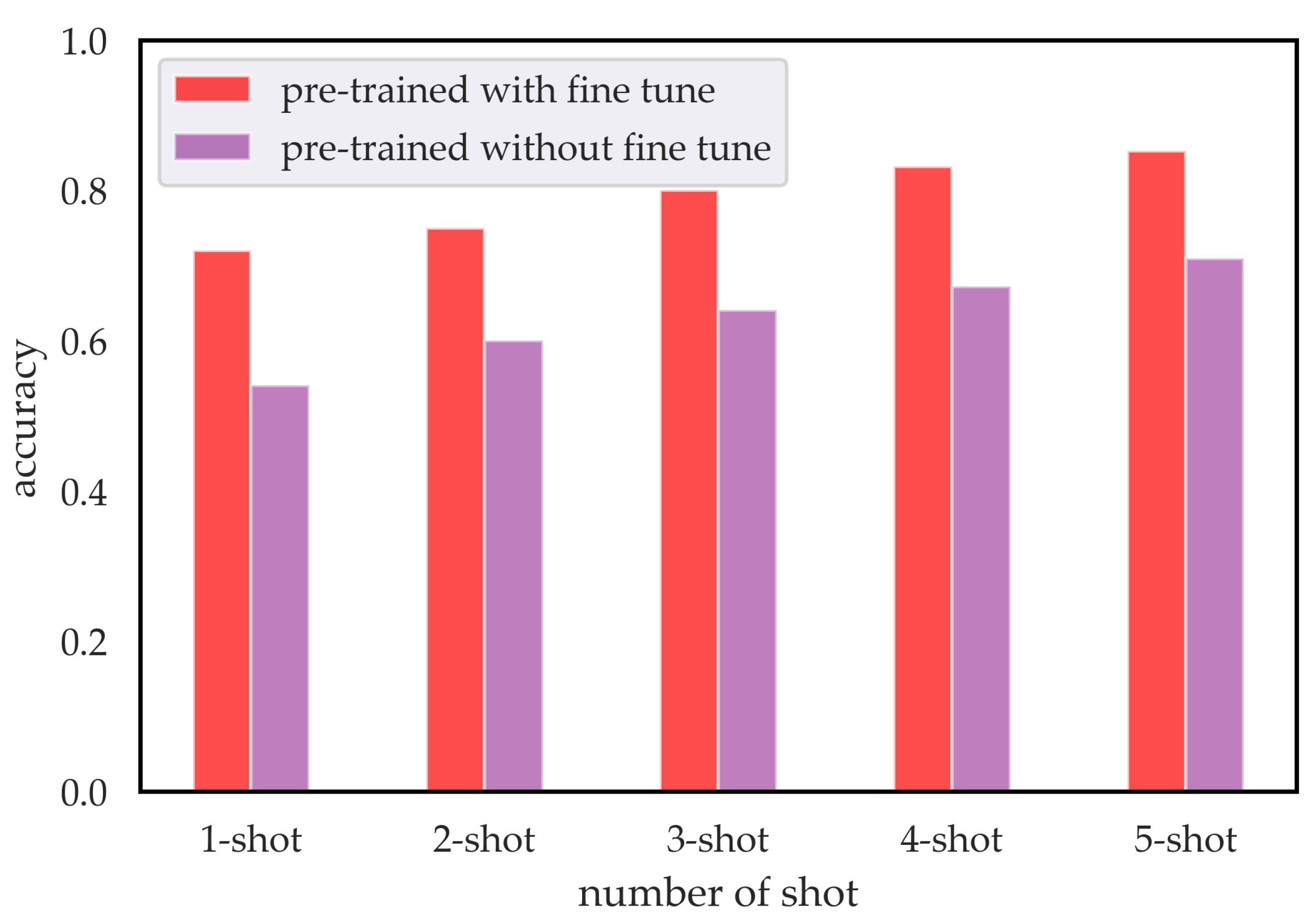
3.2.2. Fine Tuning with Sample Shuffle

After optimizing the feature encoder through numerous rounds, the deep model has the ability of feature extraction. Fine tuning is developed to improve the relevance between categories, where samples with corresponding labels are randomly shuffled. The shuffled samples are utilized to fine-tune the feature extractor, which are fused with the original samples. The function to fuse the shuffled sample and the original sample is written as below
x c = ( 1 λ ) · x + λ · x s
where x c denotes the fused sample, x stands for the original sample, x s stands for the shuffled sample, and λ is the fused parameter.
In order to enhance the robustness of the feature extractor, the fused samples x c are imported to the deep model for fine tuning. The loss L can be calculated as follows:
L = ( 1 λ ) · f L ( y p , y ) + λ · f L ( y p , y s )
where f L denotes the cross entropy function [46], y p stands for the predicted result from the network corresponding to the fused sample x c , y represents the original label of x, and y s means the shuffled label of x s . Using this loss function, relations between y and y s can be extracted, which aims to enhance the relevance of features between categories.
The overall feature encoder is optimized based on generalizing loss and then fine tuned with sample shuffle. Through generalizing loss, the feature encoder is able to extract features from remote sensing images. Furthermore, fine tuning with sample shuffle can subsequently enhance the robustness of the feature encoder, in which relations between categories tend to be included in the features.

3.3. Self-Attention Layers

In remote sensing image scene classification, images of different categories may have consistent backgrounds, which seriously affects the classification performance. Thus, background interference should be solved during feature learning. In this work, we introduce two ideas to strengthen the feature expression, one is to add self-attention layers, and the other is to deepen network layers. Self-attention layers are developed to enhance the object information, which aims to reduce the impact of background. At the same time, in order to deepen the layer of the feature encoder, skip connection is introduced to construct residual convolutional blocks.

3.3.1. Self-Attention

Remote sensing images are generally composed of foreground and background. For scene classification, background information of remote sensing images may introduce interference, which influences the performance of few-shot scene classification. In order to address this problem, self-attention layers are developed to strengthen the foreground information and weaken the background information. The self-attention module consists of three convolutional layers, where the structure is shown in Figure 3.
As shown in Figure 3, the input features with the shape of B × T × W × H are extracted from the feature extractor, where B means the batch size, T stands for the channel, W represents the width, and H represents the hight. The features are reshaped to B × T × D by the transformation operation, where D is equal to W × H . Self-attention map is a three-dimensional vector, where the first two values denote the position of the pixel, and the third value stands for the attention weight. Followed by [47], each input has its own query q i , key k i and value v i , and thus the attention map is multiplied by q i and k i and normalized by a softmax function as below
a i = e x p ( q i · k i T ) e x p ( q i · k i T ) , 1 i C × K
where a i denotes the attention map. Thus, the self-attention features can be obtained by multiplying with the attention map, which is defined as follows:
f a i = a i · v i , 1 i C × K
where f a i denotes the self-attention features, which makes the target information more salient and reduces the impact of background.

3.3.2. Residual Self-Attention

In few-shot classification, gradient explosion or gradient vanishing may appear with the increase in network depth. To resolve this issue, skip connection is applied in the proposed network, whose core idea is to calculate the output by a linear superposition and a nonlinear transformation of the input data. The function of skip connection is listed as follows
f ¯ ( x ) = f E ( x ) + x
where x stands for the input image, and f E ( · ) denotes the feature encoder, which is composed of several convolutional layers. It is obvious that features from different layers are directly added to the final output, where features of higher layer can be regarded as fitting residual features of the earlier layers.
Therefore, we construct the residual self-attention module by combining skip connection and self-attention, which is applied for feature learning. The overall formula is as follows:
R f a i = f a i + f ¯ ( x i ) , 1 i C × K
where R f a i denotes the residual self-attention features, f a i means self-attention features, and f ¯ ( x i ) stands for original features extracted with skip connection. Therefore, the overall framework of our feature encoder is depicted in Figure 4.

3.4. Prototype Calibration with Feature Generation

In few-shot remote sensing image scene classification, it may lead to a large deviation in the determination of the category prototype, since a quite limited number of labeled images can be utilized, especially when there is only one support image of each category. Therefore, we consider making full use of prior knowledge (prototype and covariance on the training set as the benchmark) to expand the support samples, and then using the forward-predicted results to calibrate the prototype of each category.

3.4.1. Feature Generation

Having limited labeled samples leads to the absence of prior knowledge. In order to take full advantage of information of labeled samples, feature generation is developed based on the characteristics of the training data. During the testing, mean and covariance of features for each category should be calculated firstly, and the mean of features denotes the prototype of each category. The calculation function [48] can be defined as follows:
μ i = j = 1 N i R f a j N i
Σ i = 1 N i 1 j = 1 N i ( R f a j μ i ) ( R f a j μ i ) T
where μ i denotes the prototype of the ith category, Σ i stands for the covariance of the ith category, N i represents the sample number of the ith category, and R f a j stands for the extracted feature corresponding to x i .
Afterwards, to enhance the performance of the proposed deep model, feature generation is developed to yield a certain number of features corresponding to the support set. That is to say, the support set of the testing set is extended by feature generation, which is based on prototypes and covariances of each category feature. For each category of the support set, we calculate the prototype of each category on the support set firstly and then select the closest prototypes of the training set based on the Euclidean distance. After that, prototype and covariance of these selected categories are utilized as the benchmark for feature generation, which can be obtained as below
μ i ¯ = R f a i + j = 1 M μ j 1 + M
Σ i ¯ = j = 1 M Σ j M + α
where μ i ¯ and Σ i ¯ stand for the mean and covariance of the benchmark, respectively, and μ j is the jth closest prototype of the training set and Σ j is the corresponding covariance. α denotes the covariance parameter, and M stands for the number of the selected prototypes from the training set.
After the benchmark of mean features and variances are obtained, features of the testing set can be extended. Suppose each dimension of features obeys Gaussian distribution, a certain number of features can be generated to extend the support set of the testing set.

3.4.2. Prototype Calibration

The prototype of each category reflects consistent features of remote sensing images, which is of great signification for few-shot classification. At the same time, prototypes of different categories have relevance, which means the prototype of a category can be transferred to other categories.
In order to strengthen the expression ability of prototypes, prototype calibration is proposed to make full use of the knowledge on the expanded support set. There is some prior knowledge on the expanded support set, which can be used to classify unlabeled samples. Considering the relevances of prototypes of different categories, we utilize the expanded support set to re-train the classifier, and the classifier is applied to predict the labels of the query set. Features corresponding to samples with high prediction probabilities are selected to calibrate the prototypes. The formula of prototype calibration can be defined as follows
μ i ^ = ( 1 β ) μ i ¯ + β j = 1 U R f a j U
where μ i ^ denotes the calibrated prototype, and μ i ¯ denotes the previously obtained prototype. R f a i stands for features of the selected sample on the query set, U denotes the number of selected samples, and β is the balance factor.
After calibrating all the prototypes of the support set, the re-trained logic regression (LR) classifier and the expanded support set are applied for few-shot classification, and labels of the query set can be predicted. Using prototype calibration with feature generation, it is able to modify prototypes in global view, which has a great contribution for few-shot remote sensing image scene classification.

4. Results and Discussions

In this section, we evaluate our proposed method on two public datasets for few-shot remote sensing image scene classification, and experimental results are reported as follows.

4.1. Dataset

NWPU-RESISC45 dataset [49] is an available benchmark for remote sensing image scene classification, which is created by Northwestern Polytechnic University. The dataset contains 31,500 images with 256 × 256 pixels, including 45 scene categories and 700 images of each category. The categories include airplane, airport, baseball field, basketball court and other scenarios. The whole dataset is divided into three subsets: training set with 25 categories, validation set with 10 categories, and testing set with 10 categories. In order to fit our designed feature encoder for feature extraction, all the images are reshaped into 84 × 84 .
The WHU-RS19 dataset [50] is also an available benchmark for remote sensing image scene classification, which is released by Wuhan University. It contains 19 categories of scene images. For each category, the sample number is greater or equal to 50, and the total number of the dataset is 1005. The whole dataset is divided into three subsets: a training set with nine categories, a validation set with five categories, and testing set with five categories. In the experiments, all the images are also reshaped to 84 × 84 to fit our designed feature encoder. Details of the two public datasets are reported in Table 1.

4.2. Parameter Setting

In the pre-training process, the weighted parameter γ is set to 0.4 , and the parameter λ is also set to 0.4 . In self-attention layers, the kernel size of convolutional layers is 1 × 1 , and the residual network is utilized as our feature encoder. Structure and parameters of the feature encoder are reported in Figure 5. In prototype calibration part, the number of the selected prototypes M is set to 2, the number of selected samples on the query set U is set to 3, and the balance factor β is set to 0.5 . In addition, logic regression (LR) is utilized as the classifier, whose max iteration is set to 1000. Hyper-parameters are selected based on the experience, which follows the related research of scene classification based on deep neural networks [18]. We utilize the PyTorch framework to implement the proposed prototype calibration with the feature-generating model, which is ran on NVIDIA GeForce RTX 2080Ti GPU and Intel(R) Xeon(R) Silver 4114 CPU.

4.3. Experimental Results on NWPU-RESISC45 Dataset

Few-shot scene classification results on the NWPU-RESISC45 data are reported in Table 2, in which accuracies are calculated by averaging the results of 600 episodes randomly generated on the testing set. In the experiments, seven other few-shot scene classification methods are utilized for comparison, where averaged results are reported. From the table, it is clearly seen that our proposed network performs best with accuracies of 85.07% and 72.05% in the cases of five-way five-shot and five-way one-shot, exceeding the accuracies of DLA-MatchNet with 3.44% and 3.25% improvements, respectively. Compared with Relation Network, the proposed network has 6.45% and 5.70% improvements in five-way one-shot and five-way five-shot, respectively. Moreover, our proposed method surpasses Meta-SGD with 9.25% improvement in five-way five-shot case and 11.39% improvement in five-way one-shot case, respectively. In addition, our proposed method yields higher accuracies than other compared approaches. Therefore, it can be demonstrated that the proposed approach can make full use of limited information from few-shot data, which improves the performance of remote sensing image scene classification.
The proposed model is able to enhance the feature representation through prototype calibration, which overcomes the deviation of prototypes caused by a small number of labeled samples. In addition, self-attention is developed for feature extraction, which reduces the influence of background information.

4.4. Experimental Results on WHU-RS19 Dataset

Experimental comparisons are also conducted on WHU-RS19 dataset, and the results are reported in Table 3. All the results are obtained with 600 episodes iteration. It is observed that the proposed few-shot classification method yields the accuracy of 72.41% and 85.26% in five-way one-shot case and five-way five-shot case, respectively. From Table 3, we can find that the proposed deep network yields superior accuracies over DLA-MatchNet, with 4.14% improvement in five-way one-shot case and 5.37% improvement in five-way five-shot case.
Compared with the results of the five-way one-shot case with the fie-way five-shot case, the performance is superior in the setting of five-way five-shot, which indicates the significance of prior knowledge. In the proposed method, prototype calibration enhances the representation ability of prototypes, which can excavate more effective prior knowledge from few-shot remote sensing images. Therefore, the proposed approach improves the accuracy of few-shot remote sensing image scene classification.

4.5. Ablation Study

To better analyze our proposed model on few-shot remote sensing image scene classification, we conduct an ablation study to analyze the effect of each module of our proposed model, which is reported as follows.

4.5.1. Effect of Pre-Training Strategy

In our pre-training strategy, fine tuning is developed to improve relevance between categories. To demonstrate the effect of fine tuning, experiments with and without fine tuning are compared and analyzed, where multiple cases with different number of shots are set for comparison. Results on the NWPU-RESISC45 dataset are depicted in Figure 6.
It can be seen from Figure 6 that the accuracy of five-way five-shot is only 70.94% without fine tuning, which is obviously lower than our model by about 14%. Similarly, in the setting of five-way one-shot, accuracy without fine tuning is 54.06%, which is lower than our model about 18%. The proposed model with fine tuning yields higher accuracies in different number of shots. It is verified that fine tuning utilized in our pre-training strategy has a great contribution to improve classification performance, which can train the feature encoder with strong ability to extract features.

4.5.2. Effect of Self-Attention Layers

In our proposed model, self-attention layers are developed to enhance the target information and reduce the influence of background. To prove the effect of self-attention, the proposed network with self-attention layers and without self-attention layers are compared on two datasets. The compared results are shown in Table 4.
It can be seen from the results that the proposed network with self-attention yields higher accuracies in the case of five-way one-shot, with about 2% improvement over the network without self-attention layers. This result indicates that self-attention has a contribution to few-shot remote sensing image scene classification, since it reduces the influence of irrelevant information for classification.

4.5.3. Discussions of Parameters for Feature Generation

Before prototype calibration, feature generation is developed to yield a certain number of features corresponding to the support set. Parameters for feature generation are discussed in this subsection. In feature generation, the closest prototypes of the training set are selected as the benchmark for feature generation, where the number of the closest prototypes is a hyper-parameter. Accuracies with different number of selected prototypes are depicted in Figure 7, where the number ranges from 1 to 7.
It is clearly seen from the results that, in the five-way one-shot case, accuracies achieve the highest on the both NWPU-RESISC45 dataset and WHU-RS19 dataset in the condition of selecting two closest prototypes. In five-way five-shot case, accuracies also become optimal when the number of selected prototypes is set to two. Therefore, two closest prototypes in the training set are selected for feature generation in the experiments.
After prototype selecting, mean and covariance of these selected prototypes are calculated as the benchmark for feature generation, where a parameter α is utilized in the calculation. In order to analyze the influence of α , classification accuracies with the changing of α in five-way one-shot case are tested on WHU-RS19 and NWPU-RESISC45 dataset. Curves of classification accuracies changing with the parameter α are shown in Figure 8.
It can be seen from Figure 8 that few-shot classification accuracy achieves the best results when α = 0 . When α is greater than 0, the accuracy decreases with the increasing of α , and the decrease is especially obvious from α = 0 to α = 0.1 . This indicates that there is no need to modify the covariance by the parameter α , at the same time; it also illustrates that covariances between the testing set and the selected prototypes of the training set are similar.

4.5.4. Effect of Prototype Calibration

In our model, prototype calibration is proposed to enhance the representative ability of different categories. To verify the effectiveness of prototype calibration, few-shot classification comparisons with different prototype calibration strategies are performed. Experimental results of different prototype calibration strategies are shown in Figure 9, where U = 0 can be regarded as the model without prototype calibration, and cases of U greater than 0 can be regarded as the model with prototype calibration.
As shown in Figure 9, the accuracy with U = 0 is the lowest, which demonstrates that the proposed prototype calibration contributes to improving the classification performance. The accuracy increases with the increasing of U, and it tends to be stable when U is larger than 5. It can be concluded that prototype calibration with five selected images from the query set is able to strengthen the expression ability of prototypes, where five images with the highest prediction probabilities are selected. Therefore, during prototype calibration, five selected images from query set are utilized to adjust prototypes, which can not only enhance the few-shot classification accuracy but also rationally use the computing resources.

4.5.5. Effect of Feature Generation

In order to illustrate the effect of feature generation, comparisons with different feature generation strategies are performed in Figure 10. Accuracies with the increasing of generated features are tested in the case of five-way one-shot. When the number of generated features is equal to 0, it can be regarded as the model without feature generation. Furthermore, cases with the number of generated features greater than 0 can be regarded as the model with feature generation.
It is observed that the accuracy increases steadily with the increasing of generated samples, and the accuracy is the lowest when the number is equal to 0, which demonstrates that feature generation can improve the classification performance. Feature generation has the ability to alleviate the impact of lack of prior information in few-shot remote sensing image scene classification. To better understand the effect of feature generation, we visualize the embeddings of support set, query set, and expanded support set, which can be found in Figure 11. It can be seen that feature distributions of the expanded support set and the query set are similar. Therefore, 500 features are generated in our model to improve the few-shot classification performance.

4.5.6. Overview

After the above experiments of the ablation study, we made the following comparisons, where composite scenarios were compared to verify the effectiveness of the proposed model. Six composite cases are compared with our overall model in Table 5, where F G denotes the deep model only with feature generation, P C denotes the deep model only with prototype calibration, S A denotes the deep model only with self-attention, S A + P C denotes the deep model with self-attention and prototype calibration, S A + F G denotes the deep model with self-attention and feature generation, and P C + F G denotes the deep model with prototype calibration and feature generation.
From the experimental results in Table 5, it is observed that the proposed model combining self-attention, prototype calibration, and feature generation achieves the highest classification accuracy. Moreover, the proposed model with prototype calibration and feature generation is slightly worse than our overall framework, which indicates that the proposed prototype calibration with the feature-generating module makes a great contribution to improving few-shot remote sensing image scene classification. The explanation for the results is that prototype calibration can effectively modify the deviation of prototypes when only a few samples are available, and feature generation can make full use of prior knowledge to expand the support set. In summary, the proposed prototype calibration with the feature generation model performs optimally in both five-way five-shot and five-way one-shot cases.

5. Conclusions

In this paper, a prototype calibration with a feature-generating model is proposed for few-shot remote sensing image scene classification. Experiments on two datasets demonstrate that the proposed method can yield superior few-shot classification results. In our proposed framework, prototype calibration module is proven to enhance the expression ability of prototype features, and feature generation can make full use of prior knowledge to expand the support set. Moreover, self-attention layers are verified to reduce the influence of irrelevant information on few-shot classification, and the pre-training strategy is effective to train a robust feature encoder.
In few-shot remote sensing image scene classification, mislabeled samples have a great influence on the classification. Understanding how to overcome the influence of mislabeled samples is an interesting research point that will be researched in the future.

Author Contributions

Conceptualization, Q.Z. and J.G. (Jie Geng); methodology, Q.Z. and J.G. (Jie Geng); software, Q.Z. and K.H.; validation, Q.Z. and J.G. (Jie Geng); formal analysis, J.G. (Jie Geng); investigation, Q.Z. and J.G. (Jie Geng); data curation, Q.Z.; writing—original draft preparation, Q.Z. and J.G. (Jie Geng); writing—review and editing, J.G. (Jie Geng), W.J. and J.G. (Jun Guo); supervision, J.G. (Jie Geng). All authors have read and agreed to the published version of the manuscript.

Funding

This research was supported by National Natural Science Foundation of China under Grant 61901376, Project funded by China Postdoctoral Science Foundation under Grant 2021TQ0271, the national undergraduate innovation and entrepreneurship training program, and Peak Experience Plan in Northwestern Polytechnical University.

Institutional Review Board Statement

Not applicable.

Informed Consent Statement

Not applicable.

Conflicts of Interest

The authors declare no conflict of interest.

References

  1. Yao, X.; Feng, X.; Han, J.; Cheng, G.; Guo, L. Automatic Weakly Supervised Object Detection From High Spatial Resolution Remote Sensing Images via Dynamic Curriculum Learning. IEEE Trans. Geosci. Remote Sens. 2021, 59, 675–685. [Google Scholar] [CrossRef]
  2. Huang, X.; Han, X.; Ma, S.; Lin, T.; Gong, J. Monitoring ecosystem service change in the City of Shenzhen by the use of high-resolution remotely sensed imagery and deep learning. Land Degrad. Dev. 2019, 30, 1490–1501. [Google Scholar] [CrossRef]
  3. Zhu, Q.; Zhong, Y.; Zhang, L.; Li, D. Adaptive deep sparse semantic modeling framework for high spatial resolution image scene classification. IEEE Trans. Geosci. Remote Sens. 2018, 56, 6180–6195. [Google Scholar] [CrossRef]
  4. Fang, B.; Li, Y.; Zhang, H.; Chan, J.C.W. Semi-Supervised Deep Learning Classification for Hyperspectral Image Based on Dual-Strategy Sample Selection. Remote Sens. 2018, 10, 574. [Google Scholar] [CrossRef] [Green Version]
  5. Othman, E.; Bazi, Y.; Melgani, F.; Alhichri, H.; Alajlan, N.; Zuair, M. Domain adaptation network for cross-scene classification. IEEE Trans. Geosci. Remote Sens. 2017, 55, 4441–4456. [Google Scholar] [CrossRef]
  6. Chaib, S.; Liu, H.; Gu, Y.; Yao, H. Deep feature fusion for VHR remote sensing scene classification. IEEE Trans. Geosci. Remote Sens. 2017, 55, 4775–4784. [Google Scholar] [CrossRef]
  7. Alajaji, D.; Alhichri, H.S.; Ammour, N.; Alajlan, N. Few-Shot Learning For Remote Sensing Scene Classification. In Proceedings of the Mediterranean and Middle-East Geoscience and Remote Sensing Symposium, Tunis, Tunisia, 9–11 March 2020; pp. 81–84. [Google Scholar]
  8. Noothout, J.M.H.; De Vos, B.D.; Wolterink, J.M.; Postma, E.M.; Smeets, P.A.M.; Takx, R.A.P.; Leiner, T.; Viergever, M.A.; Išgum, I. Deep Learning-Based Regression and Classification for Automatic Landmark Localization in Medical Images. IEEE Trans. Med. Imaging 2020, 39, 4011–4022. [Google Scholar] [CrossRef]
  9. Cen, F.; Wang, G. Boosting Occluded Image Classification via Subspace Decomposition-Based Estimation of Deep Features. IEEE Trans. Cybern. 2020, 50, 3409–3422. [Google Scholar] [CrossRef] [Green Version]
  10. Liu, Y.; Zhong, Y.; Fei, F.; Zhang, L. Scene semantic classification based on random-scale stretched convolutional neural network for high-spatial resolution remote sensing imagery. In Proceedings of the IEEE International Geoscience and Remote Sensing Symposium, Beijing, China, 10–15 July 2016; pp. 763–766. [Google Scholar]
  11. Wu, B.; Meng, D.; Zhao, H. Semi-Supervised Learning for Seismic Impedance Inversion Using Generative Adversarial Networks. Remote Sens. 2021, 13, 909. [Google Scholar] [CrossRef]
  12. Geng, J.; Deng, X.; Ma, X.; Jiang, W. Transfer Learning for SAR Image Classification Via Deep Joint Distribution Adaptation Networks. IEEE Trans. Geosci. Remote Sens. 2020, 58, 5377–5392. [Google Scholar] [CrossRef]
  13. Chang, H.; Yeung, D.Y. Semisupervised metric learning by kernel matrix adaptation. In Proceedings of the International Conference on Machine Learning and Cybernetics, Guangzhou, China, 18–21 August 2005; Volume 5, pp. 3210–3215. [Google Scholar]
  14. Shao, L.; Zhu, F.; Li, X. Transfer Learning for Visual Categorization: A Survey. IEEE Trans. Neural Netw. Learn. Syst. 2015, 26, 1019–1034. [Google Scholar] [CrossRef] [PubMed]
  15. Xu, Z.; Cao, L.; Chen, X. Learning to Learn: Hierarchical Meta-Critic Networks. IEEE Access 2019, 7, 57069–57077. [Google Scholar] [CrossRef]
  16. Xu, X.; Li, W.; Xu, D. Distance Metric Learning Using Privileged Information for Face Verification and Person Re-Identification. IEEE Trans. Neural Netw. Learn. Syst. 2015, 26, 3150–3162. [Google Scholar] [CrossRef] [PubMed]
  17. Ma, H.; Yang, Y. Two Specific Multiple-Level-Set Models for High-Resolution Remote-Sensing Image Classification. IEEE Geosci. Remote Sens. Lett. 2009, 6, 558–561. [Google Scholar]
  18. Wang, Q.; Liu, S.; Chanussot, J.; Li, X. Scene Classification with Recurrent Attention of VHR Remote Sensing Images. IEEE Trans. Geosci. Remote Sens. 2019, 57, 1155–1167. [Google Scholar] [CrossRef]
  19. Liu, S.; Deng, W. Very deep convolutional neural network based image classification using small training sample size. In Proceedings of the 3rd IAPR Asian Conference on Pattern Recognition, Kuala Lumpur, Malaysia, 3–6 November 2015; pp. 730–734. [Google Scholar]
  20. Li, L.; Han, J.; Yao, X.; Cheng, G.; Guo, L. DLA-MatchNet for Few-Shot Remote Sensing Image Scene Classification. IEEE Trans. Geosci. Remote Sens. 2020, 1–10. [Google Scholar] [CrossRef]
  21. Li, H.; Cui, Z.; Zhu, Z.; Chen, L.; Zhu, J.; Huang, H.; Tao, C. RS-MetaNet: Deep Metametric Learning for Few-Shot Remote Sensing Scene Classification. IEEE Trans. Geosci. Remote Sens. 2020, 1–12. [Google Scholar] [CrossRef]
  22. Jiang, W.; Huang, K.; Geng, J.; Deng, X. Multi-Scale Metric Learning for Few-Shot Learning. IEEE Trans. Circuits Syst. Video Technol. 2021, 31, 1091–1102. [Google Scholar] [CrossRef]
  23. Reitmaier, T.; Calma, A.; Sick, B. Transductive active learning—A new semi-supervised learning approach based on iteratively refined generative models to capture structure in data. Inf. Sci. 2015, 293, 275–298. [Google Scholar] [CrossRef]
  24. Geng, J.; Ma, X.; Fan, J.; Wang, H. Semisupervised Classification of Polarimetric SAR Image via Superpixel Restrained Deep Neural Network. IEEE Geosci. Remote Sens. Lett. 2018, 15, 122–126. [Google Scholar] [CrossRef]
  25. Wang, Y.; Xu, C.; Liu, C.; Zhang, L.; Fu, Y. Instance Credibility Inference for Few-Shot Learning. In Proceedings of the IEEE/CVF Conference on Computer Vision and Pattern Recognition, Seattle, WA, USA, 13–19 June 2020; pp. 12833–12842. [Google Scholar]
  26. Zhang, B.; Leung, K.C.; Li, X.; Ye, Y. Learn to abstract via concept graph for weakly-supervised few-shot learning. Pattern Recognit. 2021, 117, 107946. [Google Scholar] [CrossRef]
  27. Coskun, H.; Zia, M.Z.; Tekin, B.; Bogo, F.; Navab, N.; Tombari, F.; Sawhney, H. Domain-Specific Priors and Meta Learning for Few-Shot First-Person Action Recognition. IEEE Trans. Pattern Anal. Mach. Intell. 2021, 1. [Google Scholar] [CrossRef] [PubMed]
  28. Finn, C.; Abbeel, P.; Levine, S. Model-agnostic meta-learning for fast adaptation of deep networks. In Proceedings of the International Conference on Machine Learning, Sydney, NSW, Australia, 6–11 August 2017; pp. 1126–1135. [Google Scholar]
  29. Vinyals, O.; Blundell, C.; Lillicrap, T.; Wierstra, D. Matching networks for one shot learning. Proc. Neural Inf. Process. Syst. 2016, 29, 3630–3638. [Google Scholar]
  30. Sugiyarto, A.W.; Abadi, A.M. Prediction of Indonesian Palm Oil Production Using Long Short-Term Memory Recurrent Neural Network (LSTM-RNN). In Proceedings of the 1st International Conference on Artificial Intelligence and Data Sciences, Ipoh, Malaysia, 19 September 2019; pp. 53–57. [Google Scholar]
  31. Ye, Q.; Yang, X.; Chen, C.; Wang, J. River Water Quality Parameters Prediction Method Based on LSTM-RNN Model. In Proceedings of the Chinese Control Furthermore, Decision Conference, Nanchang, China, 3–5 June 2019; pp. 3024–3028. [Google Scholar]
  32. Sung, F.; Yang, Y.; Zhang, L.; Xiang, T.; Torr, P.H.; Hospedales, T.M. Learning to compare: Relation network for few-shot learning. In Proceedings of the IEEE Conference on Computer Vision and Pattern Recognition, Salt Lake City, UT, USA, 18–23 June 2018; pp. 1199–1208. [Google Scholar]
  33. Dong, H.; Song, K.; Wang, Q.; Yan, Y.; Jiang, P. Deep metric learning-based for multi-target few-shot pavement distress Classification. IEEE Trans. Industr. Inform. 2021, 1. [Google Scholar] [CrossRef]
  34. Zhu, W.; Li, W.; Liao, H.; Luo, J. Temperature network for few-shot learning with distribution-aware large-margin metric. Pattern Recognit. 2021, 112, 107797. [Google Scholar] [CrossRef]
  35. Song, Y.; Chen, C. MPPCANet: A feedforward learning strategy for few-shot image classification. Pattern Recognit. 2021, 113, 107792. [Google Scholar] [CrossRef]
  36. Li, Y.; Zhang, P.; Xu, X.; Lai, Y.; Shen, F.; Chen, L.; Gao, P. Few-shot prototype alignment regularization network for document image layout segementation. Pattern Recognit. 2021, 115, 107882. [Google Scholar] [CrossRef]
  37. Cheng, G.; Xie, X.; Han, J.; Guo, L.; Xia, G.S. Remote Sensing Image Scene Classification Meets Deep Learning: Challenges, Methods, Benchmarks, and Opportunities. IEEE J. Sel. Top. Appl. Earth Observ. Remote Sens. 2020, 13, 3735–3756. [Google Scholar] [CrossRef]
  38. Lu, X.; Gong, T.; Zheng, X. Multisource Compensation Network for Remote Sensing Cross-Domain Scene Classification. IEEE Trans. Geosci. Remote Sens. 2020, 58, 2504–2515. [Google Scholar] [CrossRef]
  39. Cheng, G.; Yang, C.; Yao, X.; Guo, L.; Han, J. When Deep Learning Meets Metric Learning: Remote Sensing Image Scene Classification via Learning Discriminative CNNs. IEEE Trans. Geosci. Remote Sens. 2018, 56, 2811–2821. [Google Scholar] [CrossRef]
  40. Zhang, W.; Tang, P.; Zhao, L. Remote Sensing Image Scene Classification Using CNN-CapsNet. Remote Sens. 2019, 11, 494. [Google Scholar] [CrossRef] [Green Version]
  41. Sun, H.; Li, S.; Zheng, X.; Lu, X. Remote Sensing Scene Classification by Gated Bidirectional Network. IEEE Trans. Geosci. Remote Sens. 2020, 58, 82–96. [Google Scholar] [CrossRef]
  42. Pires de Lima, R.; Marfurt, K. Convolutional Neural Network for Remote-Sensing Scene Classification: Transfer Learning Analysis. Remote Sens. 2020, 12, 86. [Google Scholar] [CrossRef] [Green Version]
  43. Xie, H.; Chen, Y.; Ghamisi, P. Remote Sensing Image Scene Classification via Label Augmentation and Intra-Class Constraint. Remote Sens. 2021, 13, 2566. [Google Scholar] [CrossRef]
  44. Shi, C.; Zhao, X.; Wang, L. A Multi-Branch Feature Fusion Strategy Based on an Attention Mechanism for Remote Sensing Image Scene Classification. Remote Sens. 2021, 13, 1950. [Google Scholar] [CrossRef]
  45. Zhang, P.; Bai, Y.; Wang, D.; Bai, B.; Li, Y. Few-Shot Classification of Aerial Scene Images via Meta-Learning. Remote Sens. 2021, 13, 108. [Google Scholar] [CrossRef]
  46. Mangla, P.; Kumari, N.; Sinha, A.; Singh, M.; Krishnamurthy, B.; Balasubramanian, V.N. Charting the right manifold: Manifold mixup for few-shot learning. In Proceedings of the IEEE Winter Conference on Applications of Computer Vision, Snowmass, CO, USA, 1–5 March 2020; pp. 2218–2227. [Google Scholar]
  47. Vaswani, A.; Shazeer, N.; Parmar, N.; Uszkoreit, J.; Jones, L.; Gomez, A.N.; Kaiser, Ł.; Polosukhin, I. Attention is all you need. In Proceedings of the Neural Information Processing Systems, Long Beach, CA, USA, 4–9 December 2017; pp. 5998–6008. [Google Scholar]
  48. Yang, S.; Liu, L.; Xu, M. Free Lunch for Few-shot Learning: Distribution Calibration. In Proceedings of the International Conference on Learning Representations, Virtual Event, Austria, 3–7 May 2021. [Google Scholar]
  49. Cheng, G.; Han, J.; Lu, X. Remote Sensing Image Scene Classification: Benchmark and State of the Art. Proc. IEEE 2017, 105, 1865–1883. [Google Scholar] [CrossRef] [Green Version]
  50. Sheng, G.; Wen, Y.; Tao, X.; Hong, S. High-resolution satellite scene classification using a sparse coding based multiple feature combination. Int. J. Remote Sens. 2012, 33, 2395–2412. [Google Scholar] [CrossRef]
  51. Snell, J.; Swersky, K.; Zemel, R. Prototypical networks for few-shot learning. Proc. Neural Inf. Process. Syst. 2017, 30, 4077–4087. [Google Scholar]
  52. Li, Z.; Zhou, F.; Chen, F.; Li, H. Meta-sgd: Learning to learn quickly for few-shot learning. arXiv 2017, arXiv:1707.09835. [Google Scholar]
  53. Zhai, M.; Liu, H.; Sun, F. Lifelong Learning for Scene Recognition in Remote Sensing Images. IEEE Geosci. Remote Sens. Lett. 2019, 16, 1472–1476. [Google Scholar] [CrossRef]
Figure 1. Images collected from NWPU-RESISC45 dataset. Remote sensing images in (a) reflect intra-class consistency of these images, which are well-suited to few-shot classification; remote sensing images in (b) show large intraclass variances; and images in (c) present high similarities between categories.
Remotesensing 13 02728 g001
Figure 2. The overview of prototype calibration with feature-generating model.
Remotesensing 13 02728 g002
Figure 3. The structure of the self-attention module.
Remotesensing 13 02728 g003
Figure 4. The framework of our feature encoder with self-attention.
Remotesensing 13 02728 g004
Figure 5. Structure and parameters of the feature encoder.
Remotesensing 13 02728 g005
Figure 6. Accuracies with different shots tested on NWPU-RESISC45 dataset.
Remotesensing 13 02728 g006
Figure 7. Accuracies with different number of selected prototypes, where M denotes the number of selected prototypes. (a) shows the results of 5-way 1-shot case, and (b) shows the results of 5-way 5-shot case.
Remotesensing 13 02728 g007
Figure 8. Accuracies with the changing of α tested in the case of 5-way 1-shot.
Remotesensing 13 02728 g008
Figure 9. Accuracies with different prototype calibration strategies, where U is the number of selected images from the query set.
Remotesensing 13 02728 g009
Figure 10. Accuracies with the increasing of generated features tested in the case of 5-way 1-shot.
Remotesensing 13 02728 g010
Figure 11. t-SNE visualization of the feature distribution, (a) represents the distribution of features in the support set, (b) is the visualization of the expand support set with generating 150 features per category, (c) is the visualization of the expand support set with generating 500 features per category, and (d) denotes the feature distribution of query set.
Remotesensing 13 02728 g011
Table 1. Details of NWPU-RESISC45 dataset and WHU-RS19 dataset.
DatasetsDatasetsValidationTesting
NWPU-RESISC45Airplane; Wetland;
Baseball Diamond;
Beach; Stadium;Commerical area;Airport;
Bridge; Chaparral;Industrial area;Basketball court;
Church; Sea ice;Overpass;Circle farmland;
Sparse residential;Railway station;Forest;
Cloud; Desert;Runway;River;
Freeway; Island;Snowberg;Dense residential;
Lake; Ship;Storage tank;Ground field;
Meadow; Palace;Tennis Court;Intersection;
Mobile home park;Power station;Parking lot;
Mountain; Railway;Terrace;Mid residential;
Rectangular farmland;
Golf course; Harbor;
WHU-RS19Airport;
Bridge;
Desert;Beach;Commerical;
Football field;Farmland;Meadow;
Industrial;Forest;Pond;
Mountain;Park;River;
Parking lot;Railway station;Viaduct;
Port;
Residential;
Table 2. Classification accuracy of 5-way 1-shot and 5-way 5-shot on the NWPU-RESISC45 dataset.
Method5-Way 1-Shot5-Way 5-Shot
MatchingNet [29]37.81 ± 0.6247.35 ± 0.27
Relation Network [32]66.35 ± 0.4278.62 ± 0.37
MAML [28]48.82 ± 0.9062.31 ± 0.82
Prototypical Network [51]40.41 ± 0.8863.92 ± 0.40
Meta-SGD [52]60.66 ± 0.6675.82 ± 0.52
LLSR [53]52.03 ± 0.7672.82 ± 0.62
DLA-MatchNet [20]68.80 ± 0.7081.63 ± 0.46
Ours72.05 ± 0.7585.07 ± 0.45
Table 3. Classification accuracy of 5-way 1-shot and 5-way 5-shot on the WHU-RS19 dataset.
Method5-Way 1-Shot5-Way 5-Shot
MatchingNet [29]50.20 ± 0.8954.20 ± 0.92
MAML [28]49.32 ± 0.3264.78 ± 0.73
Relation Network [32]60.92 ± 0.7479.78 ± 0.92
Meta-SGD [52]51.66 ± 0.8264.76 ± 0.93
Prototypical Network [51]58.41 ± 0.8880.78 ± 0.40
LLSR [53]57.64 ± 0.8670.66 ± 0.52
DLA-MatchNet [20]68.27 ± 1.8379.89 ± 0.33
Ours72.41 ± 0.9185.26 ± 0.66
Table 4. Classification accuracy of 5-way 1-shot on WHU-RS19 and NWPU-RESISC45 datasets.
NWPU-RESISC45WHU-RS19
with self-attention71.95 ± 0.7672.11 ± 0.32
without self-attention69.72 ± 0.4370.25 ± 0.42
Table 5. Classification accuracy with different composite scenarios tested on NWPU-RESISC45 dataset and WHU-RS19 dataset.
Proposed MethodWHU-RS19NWPU-RESISC45
1-Shot5-Shot1-Shot5-Shot
F G 64.4582.0363.2381.54
P C 60.2471.3258.5370.76
S A 64.6675.3863.8374.64
S A + P C 65.4276.2164.2175.32
S A + F G 70.3583.8869.9383.54
P C + F G 71.4384.2171.0284.07
Ours72.4185.2672.0585.07
Publisher’s Note: MDPI stays neutral with regard to jurisdictional claims in published maps and institutional affiliations.

