Mapping the Growing Stem Volume of the Coniferous Plantations in North China Using Multispectral Data from Integrated GF-2 and Sentinel-2 Images and an Optimized Feature Variable Selection Method

Abstract

Accurate measurement of forest growing stem volume (GSV) is important for forest resource management and ecosystem dynamics monitoring. Optical remote sensing imagery has great application prospects in forest GSV estimation on regional and global scales as it is easily accessible, has a wide coverage, and mature technology. However, their application is limited by cloud coverage, data stripes, atmospheric effects, and satellite sensor errors. Combining multi-sensor data can reduce such limitations as it increases the data availability, but also causes the multi-dimensional problem that increases the difficulty of feature selection. In this study, GaoFen-2 (GF-2) and Sentinel-2 images were integrated, and feature variables and data scenarios were derived by a proposed adaptive feature variable combination optimization (AFCO) program for estimating the GSV of coniferous plantations. The AFCO algorithm was compared to four traditional feature variable selection methods, namely, random forest (RF), stepwise random forest (SRF), fast iterative feature selection method for k-nearest neighbors (KNN-FIFS), and the feature variable screening and combination optimization procedure based on the distance correlation coefficient and k-nearest neighbors (DC-FSCK). The comparison indicated that the AFCO program not only considered the combination effect of feature variables, but also optimized the selection of the first feature variable, error threshold, and selection of the estimation model. Furthermore, we selected feature variables from three datasets (GF-2, Sentinel-2, and the integrated data) following the AFCO and four other feature selection methods and used the k-nearest neighbors (KNN) and random forest regression (RFR) to estimate the GSV of coniferous plantations in northern China. The results indicated that the integrated data improved the GSV estimation accuracy of coniferous plantations, with relative root mean square errors (RMSErs) of 15.0% and 19.6%, which were lower than those of GF-2 and Sentinel-2 data, respectively. In particular, the texture feature variables derived from GF-2 red band image have a significant impact on GSV estimation performance of the integrated dataset. For most data scenarios, the AFCO algorithm gained more accurate GSV estimates, as the RMSErs were 30.0%, 23.7%, 17.7%, and 17.5% lower than those of RF, SRF, KNN-FIFS, and DC-FSCK, respectively. The GSV distribution map obtained by the AFCO method and RFR model matched the field observations well. This study provides some insight into the application of optical images, optimization of the feature variable combination, and modeling algorithm selection for estimating the GSV of coniferous plantations.

1. Introduction

Forests are the largest carbon sinks in terrestrial ecosystems and play a crucial role in the global carbon cycle [1,2]. The forest growing stem volume (GSV) is the total trunk volume of various living standing trees per unit forested area, which reflects the quality of forest resources and health of the forest ecosystem [3,4]. Accurate forest GSV measurement is vital for the dynamic monitoring of regional-scale forest carbon storage [5,6,7]. The traditional GSV measurement method often disturbs the ecological environment and is expensive and laborious [5]. Remote sensing technology has significant advantages, such as wide coverage, low cost, and high efficiency, and has been widely applied in forest GSV estimation [3,4,5,6]. However, owing to the complexity and spatial heterogeneity of forest ecosystems, forest GSV estimation by remote sensing has led to many uncertainties [8,9,10]. During the actual application of remote sensing-based GSV estimation, the remote sensing data sources, selection of feature variables, and estimation models all affect the final estimation accuracy [11,12,13,14,15].

Optical remote sensing techniques have wide coverage, mature technologies, and abundant data sources [4,8,10,14,15]. However, their application is limited by cloud coverage, data stripes, atmospheric effects, and satellite sensor errors [11,15]. Microwave remote-sensing technology can penetrate the forest canopy and interact with tree trunks [16]. However, the signals are vulnerable to terrain, weather conditions, and complex forest canopy structures [17,18]. Light detection and ranging (LiDAR) data can provide vertical structure information of forests [19,20] but are less available for wide coverage due to their high cost [5,21,22]. Additionally, hyperspectral data can simultaneously image the target area on almost continuous spectral bands, which aids in capturing more forest spectral information [23]. However, the large amount of spectral information redundancy increases the computational load of data processing and applications [24]. Therefore, multispectral remote sensing imagery is still an important data source for forest GSV estimation on regional and global scales [3,8,13,25,26].

Many studies have demonstrated that the use of multi-source remote sensing data can aid in improving the GSV or aboveground biomass (AGB) estimation of forests [8,20,21,23,27,28]. Sentinel-2 is the only source of freely available optical data with four vegetation red-edge bands that are highly correlated with vegetation growth [3,4,27]. Additionally, Sentinel-2 has higher spatiotemporal resolution than MODIS and Landsat images, and greater application prospects in forest GSV estimation [3]. GaoFen-2 (GF-2) is the first civilian land-observation satellite in China, with a spatial resolution of at least 1 m [28,29]. To detect tree mortality due to the red turpentine beetle on a single tree-scale, Zhan et al. [29] evaluated the classification accuracies of GF-2 and Sentinel-2 imagery at different spatial resolutions, and their results showed that the GF-2 images had the best classification result, with an overall accuracy of 77.7%. Zhu et al. [28] integrated GF-2 optical, GF3 SAR, and UAV data to estimate the aboveground biomass of China’s largest artificially planted mangroves and found that GF-2 optical images could be used to monitor the AGB of mangrove plantations. Li et al. [13] estimated the growing stem volume of Chinese pine and larch plantations using fused optical data from GF2 and Landsat 8 imagery, and their results showed that their multispectral fusion image improved the GSV estimation accuracy better than the GF-2 and Landsat 8 images. However, no studies have estimated the GSV of conifer plantations in temperate monsoon-climate regions by combining GF-2 and Sentinel-2 imagery.

Various feature factors can be used as candidate feature variables for forest parameters estimation [13,23,30,31], including vegetation indices, image texture features, terrain factors, and phenological factors. Using a large number of feature variables can increase the possibility of improving the accuracy of the estimation model; however, it will also increase the computational load, data noise, and interference [23]. Therefore, feature selection is particularly important for forest parameters estimation [13,32]. There are two main types of feature selection methods for forest GSV estimation. (1) Feature ranking based on feature relevance or importance [23,33,34], which can quickly rank various features [35,36]. For example, the Pearson method of SciPy can simultaneously calculate the correlation coefficient and p-value; however, this method is only sensitive to linear relationships [34]. Distance correlation overcomes the weakness of the Pearson correlation coefficient [35]. If the distance correlation coefficient of two variables is zero, they can be determined to be independent. The random forest (RF) method considers the influence of a single feature variable on the estimation accuracy of the model to select the optimal feature variables according to their importance index [24,33,36]. (2) Feature combination optimization based on the estimation model accuracy [13,24], which considers the relationship between feature variables and selects the best feature combination by calculating model estimation errors based on different feature combinations [13]. Han et al. [36] proposed a fast iterative feature selection algorithm for the K-nearest neighbors (KNN) method (KNN-FIFS) to estimate the AGB of the Daxing’an Mountain Forest in northern China, and their results show that KNN-FIFS can efficiently select the optimal feature combination from high-dimensional information and is more suitable for forest AGB estimation than stepwise multiple linear regression. Jiang et al. [24] developed a novel feature variable selection method called stepwise random forest (SRF) and found that the SRF method can effectively select the optimal variable combination, with the SRF-based model achieving the highest estimation accuracy for coniferous forest GSV estimation.

Remote sensing data at fine resolution are typically combined with field measurements of plots to generate training sample datasets for regional or stand-scale forest parameters estimation by parametric or non-parametric machine learning methods [13,23,26,30]. Parametric methods are typically based on the law of large numbers [36]. However, the number of forest GSV plots that can be manually investigated is typically limited, and it is difficult for this method to describe the complex nonlinear relationship between the forest AGB and remote sensing data as the sample size is too small [13,36]. Non-parametric machine learning methods can freely fit complex sample data into different forms of functions without assuming the sample distribution [23]. Random forest regression (RFR) is an important machine learning algorithm that uses multiple decision trees for classification or prediction [24,26]. During regression model training, the decision regression trees are independent of one another and forest GSV can be quickly estimated from the weighted average of the calculation results of multiple regression trees [26]. The KNN is a theoretically mature and relatively simple machine learning method that searches for the k-nearest samples based on the greatest similarities in the feature space [13]. As the regression estimation result of the KNN method is only related to the KNNs, it is effective for resolving the sample imbalance issues [36]. The RFR and KNN methods have been widely used to estimate forest parameters [13,37,38,39,40,41,42].

This study aims to accurately estimate the GSV of coniferous plantations in a temperate monsoon climate region using integrated data from GF-2 and Sentinel-2 images based on the proposed optimized feature variable selection method and machine learning methods.

• Integrated GF-2 and Sentinel-2 data were used to estimate forest GSV. The vegetation index and multi-scale texture factors of the images were extracted as candidate feature variables for the forest GSV estimation model.
• A variable selection method was proposed based on the combination optimization effect to achieve adaptive selection and a combination of feature variables.
• We compared six different feature variable selection methods and two estimation models and explored the best solutions for coniferous plantation GSV estimation.

2. Study Area and Data

2.1. Study Area

This study was conducted in an experimental forest farm (Wangyedian) located in southwestern Harqin, Inner Mongolia, China (Figure 1). The study area is a branch of Qilaotu Mountain at the northern foot of the Yanshan Mountains, ranging from 118°09 to 118°30E and 41°21 to 41°39N [43]. Influenced by the temperate monsoon climate, this region has an average annual temperature of 4.2 °C, annual precipitation of 300–500 mm, and an annual frost-free period of approximately 117 d. There are numerous medium-sized mountains with elevations varying between 800 and 1890 m, and the area has a total stock volume of 1.4 to 1.5 million m³. In 2004, Wangyedian experimental forest farm was listed as “experimental unit of forest cutting management reform in Inner Mongolia Autonomous Region.” The main merchantable plantation tree species include larch (Larix principis-rupprechtii and Larix olgensis) and Chinese pine (Pinus tabuliformis) [44]. There are also a small number of natural forests, including white birch and Populus alba, distributed throughout the study area.

2.2. Data Preparation

2.2.1. Field Plot Data Collection

The 37 larch field plots and 42 Chinese pine field plots were selected based on tree age, terrain, and spatial distribution (Figure 2). Fieldwork was conducted from September 20 to October 15, 2017. The central positions of the sample plots were measured using a differential global positioning system (DGPS), and they had a size of 25 × 25 m. Each plot contained only one major tree species, and the sample plots with a diameter at breast height (DBH) of over 5 cm were selected and examined. For each plot, we measured and recorded the tree height, DBH, crown base height, crown diameter, altitude, slope, aspect, air temperature, and soil moisture. The spatial distribution and tree species categories of all field plots are shown in Figure 1. The GSV of each tree in the Chinese pine and larch field plots was calculated based on the two-variable (tree height and DBH) tree GSV equations provided by the Forestry Management Agency of China (http://www.forestry.gov.cn/, Accessed on 21 January 2020). The statistical information of the GSVs observed at 79 plots is presented in

Table 1. Statistical summary of the growing stem volume (m³/ha) at the field plots.

Tree Species	Numbers of Plots	Minimum	Maximum	Mean	Standard Deviation	Coefficient of Variation (%)
Chinese pine	42	91.97	514.96	257.15	112.63	0.4380
Larch	37	87.44	405.56	211.69	81.51	0.3850
All	79	87.44	514.96	237.38	99.62	0.4197

.

2.2.2. Remote Sensing Data Collection and Pre-Processing

As shown in

Table 2. Parameter information for Gapfen-2 (GF-2) and Sentinel-2 remote sensing images.

Image Category	Image Identification	Product Level	Acquisition Date
GF-2	GF2_PMS2_E118.3_N41.6_20170905_L1A0004074551-MSS	Level 1A	2017-9-5
	GF2_PMS2_E118.3_N41.6_20170905_L1A0004074551-PAN	Level 1A	2017-9-5
	GF2_PMS2_E118.3_N41.6_20170905_L1A0004074552-MSS	Level 1A	2017-9-5
	GF2_PMS2_E118.3_N41.6_20170905_L1A0004074552-PAN	Level 1A	2017-9-5
Sentinel-2	S2A_MSIL1C_20170922T025541_N0205_R032_T50TNM_20170922T030440	Level-1C	2017-9-22
	S2A_MSIL1C_20170922T025541_N0205_R032_T50TPM_20170922T030440	Level-1C	2017-9-22

, we acquired two Sentinel-2 images of the L1-level product obtained on September 22, 2017 (https://scihub.copernicus.eu/, Accessed on 17 May 2019) and two GF-2 images captured September 5, 2017 (http://www.cresda.com/CN/, Accessed on 8 May 2019)). GF-2 satellite is a high-resolution civil land observation satellite independently developed by China. The spatial resolution of the sub satellite point can reach 0.8 m. It is equipped with two high-resolution cameras of 1-m panchromatic and 4-m multispectral images. It has the characteristics of sub meter spatial resolution, high positioning accuracy and fast attitude maneuver. It has greatly improved the satellite’s comprehensive observation efficiency, which has reached the international advanced level. The parameter information of GF-2 bands is shown in

Table 3. Parameter information of bands for the GF-2 and Sentinel-2 images used in the study.

Image Category	Bands of Images	Range or Center of Wavelength(µm)	Spatial Resolution(m)
GF-2	Band 1 Pan	0.450–0.900	1
	Band 2 Blue	0.450–0.520	4
	Band 3 Green	0.520–0.590	4
	Band 4 Red	0.630–0.690	4
	Band 5NIR	0.770–0.890	4
Sentinel-2	Band 2 Blue	0.4966	10
	Band 3 Green	0.5600	10
	Band 4 Red	0.6645	10
	Band 5 Vegetation Red Edge_1	0.7039	20
	Band 6 Vegetation Red Edge_2	0.7402	20
	Band 7 Vegetation Red Edge_3	0.7825	20
	Band 8 NIR	0.8351	10
	Band 8A Vegetation Red Edge_4	0.8648	20
	Band 11 SWIR_1	1.6137	20
	Band 12 SWIR_2	2.2024	20

. Four Sentinel-2 images with a spatial resolution of 10 m, (blue, green, red, and near-infrared) and six with a spatial resolution of 20 m (vegetation red edge (VRE), short-wave infrared (SWIR)) were selected in this study for further spectral analysis and processing (Table 3). The GF-2 panchromatic images with a spatial resolution of 1 m were fused with multispectral (blue, green, red, and near-infrared (NIR)) images with a spatial resolution of 4 m following the Gram–Schmidt method. The nearest-neighbor interpolation method was followed to resample the selected Sentinel-2 bands and fused GF-2 images in order to match the pixel size to the field sample plot size. The advanced spaceborne thermal emission and reflection radiometer global digital elevation model (ASTER GDEM) data for the study area was obtained to correct the terrain of the optical satellite images, which are freely available with a spatial resolution of 30 m (http://www.gscloud.cn/, Accessed on 8 May 2019).

3. Methods

3.1. Research Framework

To improve the GSV estimation accuracy of coniferous plantations, GF-2 and Sentinel-2 images were integrated to derive various feature variables, various feature variables were selected following the proposed feature selection method, and machine learning methods were used to construct the models (Figure 3). The adaptive feature combination and optimization program (AFCO) was proposed, which not only considers the combination optimization effect among feature variables, but also optimizes the selection of the first feature variable, error threshold, and selection of estimation model. The AFCO was compared to four methods in this study: RF, SRF, KNN-FIFS, and the feature variable screening and combination optimization procedure was based on the distance correlation coefficient and k-nearest neighbors (DC-FSCK). To validate the proposed approach, three image datasets (GF-2, Sentinel-2, and integrated GF-2 and Sentinel-2 data), and two estimation models (KNN and RFR), were examined and compared.

3.2. Feature Variable Extraction Based on Image Data

In total, 864 predictive candidate feature variables were extracted for forest GSV estimation in this study (

Table 4. Feature variables used in this study. Window sizes for extracting texture factors were 3 × 3, 5 × 5, 7× 7, 9 × 9, 11×11, and 13 × 13.

Variable Type	Variable Number	Description
Spectral variables	14	GF-2: Blue, Green, Red, NIR
		Sentinel-2: Blue, Green, Red, Vegetation Red Edge_1, Vegetation Red Edge_2, Vegetation Red Edge_3, NIR, Vegetation Red Edge_3, SWIR_1, SWIR_2
Vegetation indices	175	NDVI ij = (Band i − Band j)/(Band i + Band j) NDVI ijk = (Band i + Band j − Band k)/(Band i + Band j + Band k)
		RVI i_j= Band i/Band j
		DVI i_j= Band i/Band j
		EVI = 2.5 × (BandNir − BandRed)/(BandNir + 6 ×BandRed − 7.5 ×BandBlue + 1)
		SAVIk= (BandNir − BandRed) × (1 + n)/(BandNir + BandRed + n), n = 0.1, 0.25,0.35,0.5.
		ARVI = (BandNir − (2 × BandRed−BandBlue))/(BandNir + (2×BandRed − BandBlue))
		MSR = 0.5 × (120 × (BandNir − BandGreen) − 200 × (BandRed − BandGreen)
Texture features	672	Mean (M), Variance (V), Homogeneity (H), Contrast (Con), Dissimilarity (D), Entropy (E), Second moment (S), Correlation (Cor)
Terrain factors	3	Elevation, Slope, Aspect

). We extracted ten and four multispectral bands from the original Sentinel-2 and fused GF-2 images, respectively, and 177 vegetation indices that have been widely used in forest structure parameter estimation studies were calculated [13]. The gray-level co-occurrence matrix (GLCM) was used to measure the image texture, including the mean, variance, homogeneity, contrast, dissimilarity, entropy, second moment, and correlation [13]. The GLCM was calculated with window sizes of 3 × 3, 5 × 5, 7 × 7, 9 × 9, 11 × 11, and 13 × 13. The elevation, slope, and aspect were extracted as terrain factors from the ASTER GDEM data. The extracted feature variables were then combined with the observed sample plots GSV to generate a training sample dataset (Figure 3a).

3.3. Adaptive Feature Combination Optimization Program (AFCO) for Feature Variable Selection

3.3.1. Issues with the Currently Available Feature Combination Optimization Method

Previous studies have demonstrated that the feature combination optimization method performs better than the SMLR and RF feature selection methods for the remote sensing estimation of forest structure parameters [13,24,36]. The feature combination optimization method iteratively screens the optimal feature variables based on the minimum root mean square error (RMSE) between the measured GSV and estimated values. However, the feature combination optimization method retains the following problem.

• The determination of the first feature variable (FV1) by the existing methods is typically too simple and inaccurate, and it is not dynamically updated according to the subsequent new features. The KNN-FIFS, SRF, and DC_FSCK methods cannot consider the combined effects of the features when selecting FV1, and never change the first feature in the subsequent feature combination process [13,24,36]. FV1 cannot be dynamically updated in the feature selection process, which may cause the final selected feature combination to not be the optimal feature set.
• In the feature combination process of existing methods, the lowest RMSE value obtained from the model established based on the currently selected feature combination is typically used as the feature selection threshold and is continuously updated. However, unsatisfactory situations typically occur in the actual feature selection process. For example, the program can only select two or three feature variables; however, all of the newly added features cannot obtain an RMSE value smaller than the threshold [24,36], causing feature selection to end. The RMSE-based threshold may cause other features that would help improve the accuracy of the model to be directly discarded, thereby losing the opportunity to select the best feature combination.
• The estimation model used in the feature combination process is singular; thus, the robustness of the model estimation results cannot be improved. For example, the KNN-FIFS, DC_FSCK, and SRF methods all use only one KNN or RFR model [13,24,36]; therefore, the performance of the selected feature combination has great uncertainty when used in other estimation models.

3.3.2. Adaptive Feature Combination Optimization Program (AFCO)

The proposed AFCO feature selection algorithm is shown in Figure 3b, and the specific steps are as follows.

Step 1. Set the initial candidate feature set F to the feature variables extracted in Section 3.1 and initialize the optimal feature set Best_F as an empty set, and Best_RMSE as 500.

Step 2. Select features from candidate feature set F individually, establish the GSV estimation model based on the KNN or RFR algorithms, optimize the model hyperparameters, and follow the leave-one-out cross-validation (LOOCV) method and minimum RMSE principle to determine the minimum RMSE (Min_RMSE) in the current feature set. Traverse all of the features of the candidate feature set, sort them according to Min_RMSE, and add the feature with the smallest error (best_RMSE) to Best_F.

Step 3. Update Best_F, Best_RMSE, and candidate feature set F. Calculate the number of features in the currently selected Best_F (Num) feature set; if Num = N, delete the first feature F1 in Best_F, and reselect the optimal F1 from candidate feature set F. N can be adjusted within the range of 3–10 based on the different data and models. According to the value of Num, the threshold penalty factor λ is dynamically adjusted to ensure that the program will not prematurely end due to the large RMSE of the currently selected feature combination. If the iteration condition (best_RMSE< λ×Best_RMSE) is satisfied, then move to Step 2.

Step 4. When Num reaches the set maximum value or the iteration condition in Step 3 is not satisfied, exit the program, and Best_F is the currently selected optimal feature variable combination.

KNN-FIFS, SRF, RF, and DC_FSCK were used to select feature variables for comparison with the AFCO method.

3.4. Forest GSV Estimation Modeling Based on the Selected Feature Variables

As classic machine learning algorithms, KNN and RFR typically perform well when estimating forest structure parameters and classifying vegetation [13,24,45,46]. In the KNN-based forest GSV estimation, to predict the sample (denoted as Sample-t), the algorithm finds its k-neighbor samples (S-1, S-2, S-3, ..., S-k) based on the certain distance formula. The average GSV value of the k-neighbor samples is assigned to Sample-t, and the GSV value of Sample-t is obtained. KNN typically has several distance measurement methods, such as the Manhattan, Euclidean, Mahalanobis, and Minkowski distances [47,48].

Let feature space X be an n-dimensional real vector space R_n, $x_i$, $x_j$∈X.

$$x_i={\left(x_i{}^{\left(1\right)},x_i{}^{\left(2\right)},\dots ,x_i{}^{\left(n\right)}\right)}^T$$

(1)

$$x_j={\left(x_j{}^{\left(1\right)},x_j{}^{\left(2\right)},\dots ,x_j{}^{\left(n\right)}\right)}^T$$

(2)

The Minkowski distance of $x_i$, $x_j$ is defined as:

$$D_p\left(x_i,x_j\right)={\left({{\displaystyle \sum }}_{l=1}^n{\left|x_i{}^{\left(l\right)}-x_j{}^{\left(l\right)}\right|}^p\right)}^{\frac{1}{p}}$$

(3)

where p ≥ 1; when p = 1, it is the Manhattan distance; when p = 2, it is the Euclidean distance.

The Mahalanobis distance of $x_i$, $x_j$ is defined as:

$$D_M\left(x_i,x_j\right)=\sqrt{{(x_i-x_j)}^T{C}^{-1}\left(x_i-x_j\right)}$$

(4)

where $C$ is the sample covariance matrix, $C^{-1}$ is the inverse matrix of the sample covariance matrix, and T is the transposition of the matrix.

The distance formulas used by Han et al. [36] and Li et al. [13] for the KNN-FIFS and DC-FSCK feature selection methods were the Mahalanobis and Minkowski distances, respectively, for ease of comparison; thus, the Mahalanobis distance was used in the KNN-FIFS method and the Minkowski distance was used in the DC-FSCK and AFCO methods in this study.

The RF algorithm integrates multiple decision trees through ensemble learning [33]. Each decision tree depends on a random vector, and all random vectors are independent, but identically distributed. Based on the random vector, the feature variables and sample data of the dataset are randomly selected to generate multiple decision regression trees, and the average of the estimation results of all decision trees is finally used as the RF result.   The RF algorithm is not sensitive to multivariate collinearity and is relatively robust to missing and unbalanced data and can be well-adapted to high-dimensional feature variable datasets [24,33].

Considering the superior performance of the KNN and RFR algorithms in forest GSV estimation, this study used the selected feature variable combination to construct a forest GSV estimation model based on KNN and RFR and evaluate the model accordingly.

3.5. Model Evaluation and Application

In this study, a comprehensive evaluation method was used to evaluate the performance of the forest GSV estimation model. The main evaluation indexes included the coefficient of determination (R²), adjusted R², Pearson correlation coefficient (Corr), RMSE, relative root mean square error (RMSEr), and mean absolute error (MAE). Using the LOOCV method, sample I was used as the test sample, and the remaining n-1 samples were used to establish the forest GSV estimation model based on the k-NN or RFR algorithms, which was repeated n times, and the GSV estimation values of all samples were obtained. Finally, the evaluation indices of various models were calculated using the estimated and observed GSV value. Generally, the larger the R² value, the better the fitting effect of the model, and the smaller the RMSE and Mae, the higher the estimation accuracy.

$$R^2=1-\frac{{{\displaystyle \sum }}_{i=1}^n{\left(y_i-{\widehat{y}}_i\right)}^2}{{{\displaystyle \sum }}_{i=1}^n{\left(y_i-\overline{y}\right)}^2}$$

(5)

$$Adjusted{R}^2=1-\frac{\left(1-R^2\right)\left(n-1\right)}{n-p-1}$$

(6)

$$RMSE=\sqrt{\frac{{{\displaystyle \sum }}_{i=1}^{\mathrm{n}}{\left(y_i-{\widehat{y}}_i\right)}^2}{n-1}}$$

(7)

$$RMSEr=\frac{RMSE}{\overline{y}}$$

(8)

$$Corr=\frac{{{\displaystyle \sum }}_{i=1}^n\left({\widehat{y}}_i-\overline{{\widehat{y}}_i}\right)\left(y_i-\overline{y}\right)}{\sqrt{{{\displaystyle \sum }}_{i=1}^n{\left({\widehat{y}}_i-\overline{{\widehat{y}}_i}\right)}^2}\sqrt{{{\displaystyle \sum }}_{i=1}^n{\left(y_i-\overline{y}\right)}^2}}$$

(9)

$$MAE=\frac{1}{n}{\displaystyle \sum }_{i=1}^n\left|{\widehat{y}}_i-y_i\right|$$

(10)

Finally, the best feature variables and model were used to map the GSV of coniferous plantations in the study area.

4. Results

4.1. Selection of Key Feature Variables and Development of GSV Estimation Model

In this study, six methods, i.e., RF, SRF, KNN-FIFS, DC_FSCK, AFCO-RFR, and AFCO-KNN, were used to select feature variables from an integrated GF-2 and Sentinel-2 dataset (

Table 5. Accuracy assessment of GSV estimation (m³/ha) based on integrated GF-2 and Sentinel-2 (S2) images data from the RFR or KNN models with various feature variables selected by the RF, Scheme 3 × 3, 5 × 5, 7 × 7, 9 × 9, 11 × 11, 13 × 13).

Method	Model	Selected Variables	R2	Corr	RMSE	RMSEr (%)	MAE
RF	RFR	S2_NDVI3_8, S2_NDVI6_10, S2_VRE4_W5_M, S2_NDVI5_10_2, S2_SWIR1, S2_NDVI3_6, GF2_Red, S2_Green_W5_Con, GF2_Red_W11_E, S2_NDVI4_10_2	0.457	0.678	72.92	30.72	57.67
SRF	RFR	S2_NDVI3_8, GF2_Red_W3_M, S2_Green_W13_S, S2_SWIR2_W7_H	0.653	0.815	58.30	24.56	48.51
KNN-FIFS	KNN	GF2_Red_W13_M, GF2_Red_W3_M, S2_DVI4_5, S2_SWIR2_W9_D	0.632	0.798	60.09	25.31	48.91
DC_FSCK	KNN	GF2_Red_W13_M, S2_VRE4_W11_Cor, S2_RVI3_4, S2_RVI6_8, GF2_NIR_W13_S, GF2_NIR W11_S, GF2_Red_W5_S	0.634	0.826	59.88	25.23	48.35
AFCO-RFR	RFR	GF2_Red_W3_M, S2_Green_W13_S, S2_SWIR2_W7_H, S2_RVI2_5, S2_ SWIR2_W7_V	0.751	0.874	49.41	20.82	39.87
AFCO-KNN	KNN	GF2_Red_W13_M, S2_NIR_W5_S, S2_VRE4_W11_Cor, S2_RVI3_4, S2_RVI6_8, GF2-NIR_W13_S, GF2-NIR_W11_S, GF2_Red_W5_S,GF2_Red_W13_S	0.663	0.833	57.44	24.20	45.33

). To compare and analyze the potential of GF-2 and Sentinel-2 image data in forest GSV estimation, the AFCO-RFR and AFCO-KNN methods were followed to select feature variables for the GF-2 and Sentinel-2 datasets (

Table 6. Accuracy assessment of GSV estimation (m³/ha) based on GF-2 and Sentinel-2 (S2) image data from the RFR or KNN models with various feature variables selected by the AFCO method. W–texture window size (3 × 3, 5 × 5, 7 × 7, 9 × 9, 11 × 11, 13 × 13).

Data Scenario	Model	Selected Variables	R2	Corr	RMSE	RMSEr(%)	MAE
GF-2	RFR	Red_W3_M, Green_W3_M, Red_W13_M, Red_W9_Cor, NIR_W9_H, Red_W13_E, RVI1_2, NIR_W13_Con, Green_W9_Cor, NIR_W13_D, Red_W13_Con, Blue_W3_M	0.655	0.815	58.12	24.48	45.21
	KNN	Red_W13_M, Red_W3_M, Red_W7_H, NIR_W9_H, SAVI0.35, NIR W11_S	0.650	0.820	58.60	24.69	44.00
Sentinel-2	RFR	Red_W3_M, VRE3_W5_V, VRE1_W13_S, SWIR1_W13_V, VRE4_W13_E, Aspect, NIR_W13_Cor, SWIR1_W5_M, Slope, Elevation, SWIR2_W13_Cor, SWIR2_W13_S	0.614	0.793	61.51	25.91	48.53
	KNN	NDVI2_5, VRE4_W13_H, Red_W13_S, VRE4_W13_S, NIR_W13_S, VRE4_W11_H, VRE1_W13_S, VRE3_W13_S, VRE2_W13_S, NIR_W11_S	0.612	0.785	61.64	25.96	47.42

). The features listed in the Table 5 and Table 6 were sorted according to the chronological order in which they were selected by various methods. We developed corresponding GSV estimation models based on the selected feature variables for various data scenarios. The key hyperparameters and best configurations of the tuning parameters for each data scenario and estimation model are listed in

Table 7. Tuned hyperparameters and best configurations for each data scenario and estimation model.

Data Scenario	Feature Variable Selection Method	Model	Tuned Hyperparameters	Hyperparameter Configurations
Integrated data of GF-2 and Sentinel-2	RF	RFR	n_estimators	26
			max_features	3
	SRF	RFR	n_estimators	42
			max_features	2
	KNN-FIFS	KNN	metric, weights	Mahalanobis, distance,
			n_neighbors	2
	DC_FSCK	KNN	metric, weights	Minkowski, distance,
			n_neighbors, p	2, 1
	AFCO	RFR	n_estimators	24
			max_features	2
		KNN	metric, weights	Minkowski, distance,
			n_neighbors, p	2, 1
GF-2	AFCO	RFR	n_estimators	16
			max_features	3
		KNN	metric, weights	Minkowski, distance
			n_neighbors, p	3, 1
Sentinel-2	AFCO	RFR	n_estimators	16
			max_features	2
		KNN	metric, weights	Minkowski, distance
			n_neighbors, p	2, 2

. As shown in Table 5 and Table 6, the R², adjusted R², Corr, RMSE, RMSEr, and MAE values were used to evaluate the model estimation results obtained by LOOCV.

For the integrated GF-2 and Sentinel-2 dataset, the largest R² of 0.751 and smallest RMSEr values of 20.82% were obtained by the proposed AFCO method of this study combined with the RFR model (Table 5). The estimation accuracy was the worst when selecting feature variables following the RF method and constructing the GSV estimation model based on the RFR algorithm, with R² of 0.457 and RMSEr values of 30.72%. The estimation accuracies of the SRF, KNN-FIFS, and DC-FSCK methods combined with RFR or KNN models were similar, with RMSEr values of 24.56%, 25.31%, and 25.23%, and MAE values of 48.51, 48.91, and 48.35 m³/ha, respectively. In order to further analyze the GSV estimation ability of the feature variables selected by the AFCO-RFR method, we adopted Pearson correlation coefficient and random forest mean decrease accuracy (RF-MDA) methods to calculate the correlation and importance indicators of the variables (Figure 4, Appendix A, Figure A1 and Figure A2). The results show that GF2_Red_W3_M has the highest GSV correlation of -0.57, and the good importance index of 0.2770. Considering the correlation and importance evaluation results of features, we find that GF2_Red_W3_M has the highest GSV estimate ability, followed by S2_RVI_{2_5}.

For the GF-2 image (Table 6), the AFCO-RFR and AFCO-KNN methods selected twelve and six feature variables, respectively. As the GF-2 images do not have vegetation red edges or short-wave infrared images, most of the key feature variables selected by the AFCO method were related to the red or green bands. For the Sentinel-2 image, the AFCO-RFR and AFCO-KNN selected twelve and ten feature variables, respectively. Previous research has demonstrated that the VRE and SWIR bands are highly correlated with GSV or AGB, which can effectively improve the accuracy of estimating forest structural parameters. In this study, the AFCO-RFR and AFCO-KNN methods from the Sentinel-2 image dataset selected seven and six feature variables related to the VRE or SWIR bands, respectively. As shown in Figure 5, Red_W3_M is the feature variable with the highest importance index and correlation coefficient in both of GF-2 and Sentinel-2 datasets. It can be seen that the spectral mean information with Red band image of a 3 × 3 window size has a great contribution to GSV estimation. In conclusion, considering the correlation and importance of GSV estimation, the feature variables related to red and green bands are the most important for GF-2 images, while red, SWIR and VRE are the most important bands for sentinel-2 images.

Figure 6 and Figure 7 present the scatter plot of the observed and estimated GSV values. The residuals of the estimated GSV based on the integrated dataset was shown in Figure A3, in which the AFCO-RFR method and RFR model were employed. Compared with a single GF-2 and Sentinel-2 data set, the integrated dataset of GF-2 and Sentinel-2 images have higher GSV estimation performance. The best R² value based on the integrated dataset was 14.66%, and 22.31% higher than that of the GF-2 and Sentinel-2 dataset respectively, and the optimal RMSEr values were 14.95% and 19.64% lower, respectively. In summary, the GSV estimation performance of GF-2 is slightly higher than Sentinel-2, thus GF-2 is more critical than Sentinel-2 for the improvement of GSV estimation performance of the integrated data set.

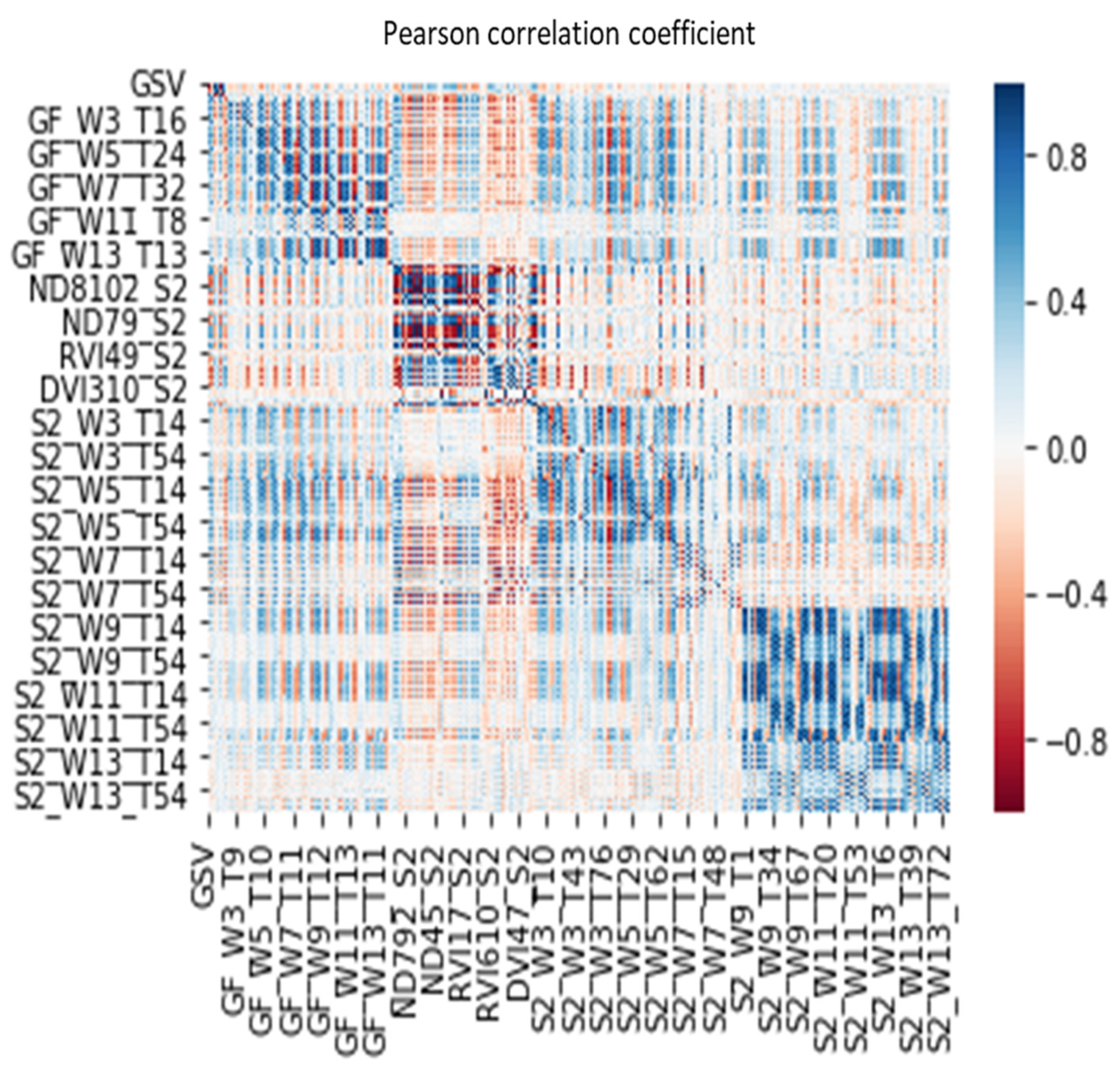
4.2. Correlation Analysis of Feature Variables

In order to find the key feature variables suitable for GSV estimation, we extracted 864 feature variables from the integrated gf-2 and sentinel-2 dataset. Because of the high similarity among a large number of features, information redundancy and multicollinearity problems will occur and bring about the instability of the regression model. Comparing the autocorrelation between features before and after feature selection (Figure A1, Figure A2 and Figure 4), we find that AFCO-RFR method significantly weakens the correlation between feature variables. As shown in Figure A1 and Figure A2, before feature selection, although many features have a strong correlation with GSV, and the strong correlation among themselves. In particular, the correlation coefficient values of various vegetation index features are very high, some even close to 1 or −1, which indicates that the information redundancy between features is very high.

The Durbin–Watson (DW) test is usually used to test the first-order autocorrelation of residuals in regression analysis [49]. Supposing that the residual is $e_t$, the correlation equation of each residual can be expressed as follows.

$$e_t=\rho \times e_t+v_t$$

(11)

The null hypothesis of the correlation test is: $\rho =0$, the test statistic is as follows.

$$DW=\frac{{{\displaystyle \sum }}_{t=2}^T{\left(e_t-e_{t-1}\right)}^2}{{{\displaystyle \sum }}_{t=1}^T{e}_t^2}$$

(12)

Savin and White (1977) present Durbin–Watson significance tables, taking sample sizes ranging from 6 to 200 with 1 to 20 regressors for models in which an intercept is included (https://www3.nd.edu/~wevans1/econ30331/Durbin_Watson_tables.pdf, Accessed on 30 June 2021). According to Savin and White‘s tables, we found that the printed bounds are dL = 1.487 and dU = 1.770 at the 5% level of significance, when the sample size is 79, and the number of independent variables is 5. By the Durbin–Watson test, we observed the value of the test statistic DW was 1.859, which was greater than the tabulated upper bound of 1.770, so we could not reject the null hypothesis of non-autocorrelated errors, which means that there is no autocorrelation at the 5% level significance among the feature variables selected by the AFCO-RFR method.

The significance statistic in multiple linear regression analysis show the influence of the independent variable on the dependent variable. Generally, a significance value less than 0.05 indicates a significant influence, and the smaller value the greater influence. Collinearity statistics can be used to judge between multiple variables whether and how much they are related to each other, the variance inflation factor (VIF) is usually used to evaluate the multicollinearity in a multiple linear regression model. The value of VIF is greater than 1, and when VIF < 10, there is no multicollinearity. As shown in

Table 8. Multiple regression analysis of feature variables selected by AFCO-RFR method for integrated GF-2 and Sentinel-2 datasets. The dependent variable is GSV. Sig., Significance, VIF, and variance inflation factor.

Predictive Variables and Intercept	Nonstandard Coefficient		Standard Coefficient	t	Sig.	Collinearity Statistics
	B	Standard Error	Beta			Tolerance	VIF
Intercept	420.141	45.194		9.296	0.000
GF2_Red_W3_M	−43.375	13.297	−0.394	−3.262	0.002	0.549	1.822
S2_RVI2_5	−480.664	245.057	−0.215	−1.961	0.054	0.668	1.497
S2_Green_W13_S	117.667	109.950	0.121	1.070	0.288	0.629	1.591
S2_SWIR2_W7_H	56.558	38.189	0.164	1.481	0.143	0.654	1.528
S2_SWIR2_W7_V	−0.294	5.223	−0.006	−0.056	0.955	0.782	1.278

, GF2_Red_W3_M has a significance value of 0.002, which is much higher than other features, which means that it has the greatest influence on the accuracy in GSV estimation model. Consistent with the conclusion in Section 4.1, this further confirms GF-2 is more important to the improvement of GSV estimation performance of the integrated data set than Sentinel-2. In addition, the obtained VIF values of all the feature variables are less than 2, showing that there is no significant multicollinearity among them.

4.3. Predicting and Mapping the GSV of Coniferous Plantation

We mapped the spatial GSV distribution of coniferous plantations using five feature variable selection methods and two models based on the integrated GF-2 and Sentinel-2 data for our study area (Figure 8a–f). Figure 8g,h show the estimated GSV distribution map obtained using the AFCO-RFR method based on GF-2 and Sentinel-2 images, respectively. Figure 8a exhibits more orange and light green areas and fewer red and blue areas. The lowest value and highest values were approximately 105 and 370 m³/ha, respectively. The results show that the estimation results based on the RF feature selection method exhibited severe overestimation and underestimation in the regions with low and high GSV values, respectively. The GSV distribution range in Figure 8b is 100–390 m³/ha, which was higher than that of the RF method; however, there were more low-value regions than the actual distribution of GSV, indicating that the method based on SRF and RFR also underestimated the actual GSV. The distribution of GSV obtained by the KNN-FIFS, DC-FSCK, AFCO-KNN, and AFCO-RFR methods (Figure 8c–f) performed better than the RF and SRF methods (Figure 8a,b) and their GSV distribution ranges were 90–495, 89–514, 87–514, and 90–499 m³/ha, respectively. In summary, the GSV map (Figure 8f) obtained using the AFCO-RFR method was the most consistent with the actual distribution of GSV, particularly in low-GSV areas that are close to residential zones.

In the area with high GSV values, the color in Figure 8f is not as dark as that in Figure 8c–e. This may be because AFCO-RFR used an ensemble learning algorithm based on multiple decision trees, which was more robust than the nearest-neighbor method based on KNN. Therefore, the estimation results of AFCO-RFR avoided extremely small and large GSV values. The GSV results estimated by the AFCO method based on GF-2 and Sentinel-2 images were shown in Figure 8g, Figure 8h, respectively. Compared with Figure 8h, Figure 8g was more similar to Figure 8f. Figure 8g,h were very different in the northwest region and the reason may be that GF-2 has higher spatial resolution. Therefore, GF-2 is more sensitive to changes in GSV. Another reason may be that the fallen leaves of the larch in this area in October led to the great uncertainty between the spectral signal of the forest canopy and forest GSV. In summary, the GSV distribution map obtained by the integrated GF-2 and Sentinel-2 data matches the field observation results better than those using GF-2 and Sentinel-2 data alone. Additionally, the saturation of the estimated GSV based on the AFCO method was 35.6% and 30.8% higher than that of the RF and SRF methods, respectively.

5. Discussion

5.1. The Importance of Feature Selection Methods in GSV Estimation

The AFCO method proposed in this study overcomes the defects of the existing feature ranking and feature combination methods, comprehensively considers the estimation performance of a single feature and the combination effect between features and has good performance in GSV modeling combining remote sensing image and field plot survey data. Compared with RF, KNN-FIFS, SRF, and DC-FSCK, the proposed AFCO method has great improvement in RMSE, MAE and R² of GSV estimation. For the GF-2 image dataset, the largest R² and smallest RMSEr values of 0.655 and 24.48% were obtained by the combination of AFCO-RFR method and RFR model. Although we did not follow a tree species stratification method to establish the GSV estimation model or use the fused images and stacking integrated algorithm, we achieved better accuracy than Li et al.‘s GSV estimation results (RMSEr of 25.72%) and used GF-2 image for a larch plantation [13], based on the Chinese pine and larch mixed samples in this study. This is due to the advantages of the AFCO method for combining feature variables.

Following the AFCO method, we used Sentinel-2 image data to select feature variables and constructed RFR and KNN models, and the RMSEr values were 25.91% and 25.96%, respectively. Jiang et al. [24] used Sentinel-2 images combined with the SRF method and RFR model to estimate coniferous plantation GSV in the same study area. Their minimum RMSEr was only 28% and the GSV estimation accuracy was significantly lower than that of the AFCO method proposed in this study. Moreover, Zhang et al. [42] achieved poor performance in estimating the AGB of evergreen needleleaf forests using multi-source data and eight machine learning regression algorithms, and the RMSEr exceeded 60%. The high RMSEr value may have been because samples with high AGB values could not be captured by the remote sensing data due to saturation issues. Additionally, they did not use high-quality feature variable selection methods.

Luo et al. [32] estimated the AGB of forests in Jilin Province, northeast China, using Ninth National Forest Continuous Inventory data and Landsat OLI images. They used recursive feature elimination for feature selection and categorical boosting as the regression algorithm, and achieved the highest accuracy for coniferous forests, with RMSE and RMSEr values of 26.54 Mg/ha and 25.62%, respectively. Although they used 358 coniferous forest field observation sample plots and tested three machine learning integrated estimation algorithms, the AGB estimation accuracy of coniferous forest was much lower than that in this study, with the smallest RMSE and RMSEr values of 49.41 m3/ha and 20.82%, respectively. The main reason for this may be that they only used a Landsat image dataset, and their feature variable selection method ignored the combined effects of variables. Jiang et al. [24] used Sentinel-2 images based on SRF methods and an RFR model to estimate the GSV of a coniferous forest, and achieved the highest GSV estimation accuracy, with an R² of 0.62 and RMSEr of 28.0%. Although they found that the SRF method performed better than the linear stepwise regression, RF, Boruta, and variable selection using RF methods, all of the model evaluation indicators of the SRF method were worse than those of the AFCO method proposed in this study. This could be due to the three improvements of the AFCO method, including the first feature selection, estimation error threshold, and estimation model selection. Long et al. [50] estimated the GSV of Chinese fir plantations using four L-band ALOS PALSAR-2 quad-polarimetric synthetic aperture radar images and a general linear model in Hunan Province, south-central China. Using the fused polarimetric characteristics and general linear model, the minimum RMSEr was 24.42% from time-series SAR images. Although the single-tree species Chinese fir plantation GSV estimation model theoretically achieved higher estimation accuracy than the mixed Chinese pine and larch GSV estimation model, and microwave images were less affected by weather conditions, the time-series quad-polarimetric SAR images should provide greater potential for obtaining higher GSV estimation accuracy than optical images. The RMSEr values of GSV estimation obtained by Long et al. [50] were much higher than those in this study, which may be because it was difficult for their method to accurately select features related to forest GSV.

5.2. GSV Estimation Performance and Key Feature Variable Analysis of GF-2 and Sentinel-2 Images

The application of the integrated GF-2 and Sentinel-2 dataset effectively improved GSV estimation accuracy in this study. By comparison, we found that the GSV estimation ability of sentinel-2 is slightly lower than that of GF-2 (Table 5), and the feature Red_W3_M of GF2 has stronger GSV estimation performance than all the feature variables in the integrated dataset (Figure 4). Therefore, compared with Sentinel-2, GF-2 images are more critical for improving the GSV estimation performance of the integrated dataset. The reason may be that GF-2 has a great advantage in spatial resolution, which has more fine texture features and more rich forest spatial details than Sentinel-2.

Due to the strong correlation between red band image of sub meter resolution GF-2 and plot GSV, the texture feature variables extracted from red band image have high GSV estimation ability (Figure 4 and Figure 5). In particular, when selecting features based on the integrated dataset of GF-2 and Sentinel-2 image using the AFCO-RFR method, the Red_W3_M of GF-2 with the highest GSV correlation was the first selected key feature variable. In addition, all the first key features selected by the six methods were related to the red band of GF-2 or Sentinel-2 image (Table 4). Li et al. [43] used ZiYuan-3 (ZY-3) multispectral and stereo data to estimate the aboveground biomass of larch plantations in northern China and found that the red band from ZY-3 was strongly correlated with the aboveground forest biomass. When the Gram–Schmidt image sharpening method was used to fuse the multispectral data of GF-2 and Landsat 8 to make GSV estimation of coniferous plantation in northern China, Li et al. found that the fusion image obtained by using the red band of GF-2 had better GSV estimation capability than that obtained by using other bands. These results indicate that the red band of the high-resolution image made a greater contribution to the estimation of forest structure parameters than the other bands.

Image-based texture factors play a more critical role in forest GSV estimation than other feature variables. Most of the variables selected by the SRF, KNN-FIFS, and DC-FSCK methods were texture features in this study. This is highly consistent with the results found by Jiang et al., who used the SRF method to select features based on Sentinel-2 images for GSV estimation. In addition, Han et al. [36] used multi-source remote sensing data to estimate forest AGB in the Daxinganling Genhe Forest Reserve of northern China and found that six variables of the eight selected by the KNN-FIFS method were texture features.

Generally, when the texture window is small, such as 3 × 3 or 5 × 5, the extracted texture factors have a better correlation with the GSV of the sample plot (Figure 5). In this study, the first key variables selected by AFCO-RFR method in the three image data scenes are the texture feature with the window size of 3 × 3. For the GF-2 data set, the first three key variables selected by AFCO-RFR method are Red_W3_M, Green_W3_M and Red_W13_M, which shows that pixel smoothing by using mean method increases the correlation between image and GSV. Interestingly, in all the selected feature variables, GF-2 and sentinel-2 have five and six texture features with window size of 13 × 13 respectively, which may be caused by a variety of factors, including the physiological characteristics of the tree species, the specific spatial distribution as well as the spatial scale effect of the image and the sample plot. However, in other study areas or other tree species, the appropriate window size of the texture features for the GSV estimation may be different.

Sentinel-2′s unique four vegetation red-edge bands are very beneficial to forest resource monitoring. In addition, the short-wave infrared band also has a good performance in GSV monitoring. As shown in Table 4 and Table 5, the AFCO-RFR method was used to select three and four feature variables related to the VRE and SWIR bands from the sentinel-2 dataset respectively, one and two feature variables from the integrated dataset of GF-2 and sentinel-2 images respectively. The feature importance index of these features is very high, and the correlation with GSV is also very strong (Figure 4 and Figure 5), indicating that they are more sensitive to the changes of forest GSV value than others.

5.3. Analysis of Factors Affecting the Accuracy of Forest GSV Estimation

Currently, the remote sensing atmospheric effect and sensor errors cannot be eliminated completely [23,26]; however, the influence of these errors can be effectively suppressed by integrating multi-sensor and time-series data [13,21,27,28]. The sampling design, sample plot selection, and field sample plot investigation time can be further improved according to forest type, forest land topography, and phenology characteristics. Previous research demonstrated that different combinations of feature variables directly affect the accuracy of model estimation results [13,36,38]. The AFCO method proposed in this study not only considers the correlation and combination effect among the feature variables, but also optimizes the selection of the first feature variable, error threshold, and estimation model selection. Therefore, the AFCO method provides a novel and effective approach for improving the GSV estimation accuracy. Additionally, model selection is also vital for improving the GSV estimation accuracy [13,36]. Relevant studies have demonstrated that the ensemble machine learning method integrating the superior performance of various models can overcome the contingency and one-sidedness caused when using the estimation results of a single model and effectively improve the estimation accuracy [10,13,31,32,51]. Therefore, in future research, we will attempt to combine the AFCO method with a stacking integration algorithm or categorical boosting algorithm to explore the effectiveness of forest GSV estimation.

6. Conclusions

In this study, a novel method (AFCO) was proposed and used to select the optimal combination of feature variables from integrated GF-2 and Sentinel-2 image data, and the results demonstrate the superiority of the AFCO method and potential of using integrated GF-2 and Sentinel-2 image data for coniferous plantation GSV estimation at regional scales. The AFCO method examines the combination effect relationship between the feature variables and optimizes the first feature variable selection, error threshold, and estimation models. Comparing the autocorrelation between features before and after feature selection, we find that the variable combination selected by using the AFCO-RFR method not only has high GSV estimation performance, but also significantly reduces the autocorrelation among variables. For the integrated GF-2 and Sentinel-2 data, the AFCO method combined with the RFR model achieved higher estimation accuracy and saturation than the other solutions. The best-adjusted R² and RMSEr values were 0.751 and 20.82%, respectively. The R² of the proposed AFCO method was 74.3%, 15.0%, 18.8%, and 18.5% higher than those of the RF, SRF, KNN-FIFS, and DC-FSCK methods, and the RMSEr values were 30.0%, 23.7%, 17.7%, and 17.5% lower, respectively. Additionally, the R² achieved based on the integrated GF-2 and Sentinel-2 data was 14.7% and 22.3% higher than those achieved using GF-2 and Sentinel-2 data alone, and the RMSErs were 15.0% and 19.6% lower, respectively. The results show that the integrated GF-2 and Sentinel-2 image data and proposed AFCO method jointly improved the forest GSV estimation accuracy. Especially, the texture feature variables of GF-2 red band image significantly improve the GSV estimation ability of the integrated dataset. This research provides new insights for forest GSV estimation research based on multi-source remote sensing images and measured sample plot data.

References

1. Sean, S.; Jeffrey, A.S. Forest resources assessment of 2015 shows positive global trends but forest loss and degradation persist in poor tropical countries. For. Ecol. Manag. 2015, 352, 134–145. [Google Scholar] [CrossRef] [Green Version]
2. UNFCCC. Report of the Conference of the Parties on Its Twenty-First Session, Held in Paris from 30 November to 13 December 2015. Addendum. Part Two: Action Taken by the Conference of the Parties at Its Twenty-First Session. 2016. Available online: http://unfccc.int/resource/docs/2015/cop21/eng/10a01.pdf (accessed on 17 April 2021).
3. Astola, H.; Hame, T.; Sirro, L.; Molinier, M.; Kilpi, J. Comparison of Sentinel-2 and Landsat 8 imagery for forest variable prediction in boreal region. Remote Sens. Environ. 2019, 223, 257–273. [Google Scholar] [CrossRef]
4. Chrysafis, I.; Mallinis, G.; Siachalou, S.; Patias, P. Assessing the relationships between growing stock volume and Sentinel-2 imagery in a Mediterranean forest ecosystem. Remote Sens. Lett. 2017, 8, 508–517. [Google Scholar] [CrossRef]
5. Lindberg, E.; Hollaus, M. Comparison of methods for estimation of stem volume, stem number and basal area from airborne laser scanning data in a hemi-boreal forest. Remote Sens. 2012, 4, 1004–1023. [Google Scholar] [CrossRef] [Green Version]
6. Wijaya, A.; Kusnadi, S.; Gloaguen, R.; Heilmeier, H. Improved strategy for estimating stem volume and forest biomass using moderate resolution remote sensing data and GIS. J. For. Res. Jpn. 2010, 21, 1–12. [Google Scholar] [CrossRef]
7. Asner, G.P.; Powell, G.; Mascaro, J.; Knapp, D.E.; Clark, J.K.; Jacobson, J.; Kennedy-Bowdoin, T.; Balaji, A.; Paez-Acosta, G.; Victoria, E.; et al. High-resolution forest carbon stocks and emissions in the Amazon. Proc. Natl. Acad. Sci. USA 2010, 107, 16738–16742. [Google Scholar] [CrossRef] [PubMed] [Green Version]
8. Puliti, S.; Saarela, S.; Gobakken, T.; Stahl, G.; Naesset, E. Combining UAV and Sentinel-2 auxiliary data for forest growing stock volume estimation through hierarchical model-based inference. Remote Sens. Environ. 2018, 204, 485–497. [Google Scholar] [CrossRef]
9. Bilous, A.; Myroniuk, V.; Holiaka, D.; Bilous, S.; See, L.; Schepaschenko, D. Mapping growing stock volume and forest live biomass: A case study of the Polissya region of Ukraine. Environ. Res. Lett. 2017, 12, 105001. [Google Scholar] [CrossRef] [Green Version]
10. Chrysafis, I.; Mallinis, G.; Gitas, I.; Tsakiri-Strati, M. Estimating Mediterranean forest parameters using multi seasonal Landsat 8 OLI imagery and an ensemble learning method. Remote Sens. Environ. 2017, 199, 154–166. [Google Scholar] [CrossRef]
11. Fassnacht, F.E.; Hartig, F.; Latifi, H.; Berger, C.; Hernández, J.; Corvalán, P.; Koch, B. Importance of sample size, data type and prediction method for remote sensing-based estimations of aboveground forest biomass. Remote Sens. Environ. 2014, 154, 102–114. [Google Scholar] [CrossRef]
12. Bogan, S.A.; Antonarakis, A.S.; Moorcroft, P.R. Imaging spectrometry-derived estimates of regional ecosystem composition for the Sierra Nevada, California. Remote Sens. Environ. 2019, 228, 14–30. [Google Scholar] [CrossRef]
13. Li, X.; Liu, Z.; Lin, H.; Wang, G.; Sun, H.; Long, J.; Zhang, M. Estimating the growing stem volume of Chinese Pine and Larch Plantations based on fused optical data using an improved variable screening method and stacking algorithm. Remote Sens. 2020, 12, 871. [Google Scholar] [CrossRef] [Green Version]
14. Dube, T.; Mutanga, O. The impact of integrating WorldView-2 sensor and environmental variables in estimating plantation forest species aboveground biomass and carbon stocks in uMgeni Catchment, South Africa. ISPRS J. Photogramm. Remote Sens. 2016, 119, 415–425. [Google Scholar] [CrossRef]
15. Granero-Belinchon, C.; Adeline, K.; Briottet, X. Impact of the number of dates and their sampling on a NDVI time series reconstruction methodology to monitor urban trees with Venμs satellite. Int. J. Appl. Earth Obs. Geoinf. 2021, 95, 102257. [Google Scholar] [CrossRef]
16. Sinha, S.; Jeganathan, C.; Sharma, L.K.; Nathawat, M.S. A review of radar remote sensing for biomass estimation. Int. J. Environ. Sci. Technol. 2015, 12, 1779–1792. [Google Scholar] [CrossRef] [Green Version]
17. Santoro, M.; Beaudoin, A.; Beer, C.; Cartus, O.; Fransson, J.E.S.; Hall, R.J.; Pathe, C.; Schmullius, C.; Schepaschenko, D.; Shvidenko, A. Forest growing stock volume of the northern hemisphere: Spatially explicit estimates for 2010 derived from Envisat ASAR. Remote Sens. Environ. 2015, 168, 316–334. [Google Scholar] [CrossRef]
18. Soja, M.J.; Quegan, S.; d’Alessandro, M.M.; Banda, F.; Scipal, K.; Tebaldini, S.; Ulander, L.M.H. Mapping above-ground biomass in tropical forests with ground-cancelled P-band SAR and limited reference data. Remote Sens. Environ. 2021, 253, 112153. [Google Scholar] [CrossRef]
19. Fu, L.; Liu, Q.; Sun, H.; Wang, S.; Li, Z.; Chen, E.; Pang, Y.; Song, X.; Wang, G. Development of a system of compatible individual tree diameter and aboveground biomass prediction models using error-in-variable regression and airborne LiDAR data. Remote Sens. 2018, 10, 325. [Google Scholar] [CrossRef] [Green Version]
20. Chen, Q.; Laurin, G.V.; Battles, J.J.; Saah, D. Integration of airborne LiDAR and vegetation types derived from aerial photography for mapping aboveground live biomass. Remote Sens. Environ. 2012, 121, 108–117. [Google Scholar] [CrossRef]
21. Zhang, Y.; Shao, Z.F. Assessing of urban vegetation biomass in combination with LiDAR and high-resolution remote sensing images. Int. J. Remote Sens. 2021, 42, 964–985. [Google Scholar] [CrossRef]
22. Cao, L.; Coops, N.C.; Innes, J.L.; Sheppard, S.R.J.; Fu, L.; Ruan, H.; She, G. Estimation of forest biomass dynamics in subtropical forests using multi-temporal airborne LiDAR data. Remote Sens. Environ. 2016, 178, 158–171. [Google Scholar] [CrossRef]
23. Lu, D.; Chen, Q.; Wang, G.; Li, G.; Moran, E. A survey of remote sensing-basedd aboveground biomass estimation methods in forest ecosystems. Int. J. Digit. Earth 2016, 9, 63–105. [Google Scholar] [CrossRef]
24. Jiang, F.; Kutia, M.; Sarkissian, A.J.; Lin, H.; Long, J.; Sun, H.; Wang, G. Estimating the Growing Stem Volume of Coniferous Plantations Based on Random Forest Using an Optimized Variable Selection Method. Sensors 2020, 20, 7248. [Google Scholar] [CrossRef]
25. Guo, Z.; Wang, T.; Liu, S.; Kang, W.; Chen, X.; Feng, K.; Zhang, X.; Zhi, Y. Biomass and vegetation coverage survey in the Mu Us sandy land-based on unmanned aerial vehicle RGB images. Int. J. Appl. Earth Obs. Geoinf. 2021, 94, 102239. [Google Scholar] [CrossRef]
26. Kumar, L.; Mutanga, O. Remote sensing of above-ground biomass. Remote Sens. 2017, 9, 935. [Google Scholar] [CrossRef] [Green Version]
27. Vafaei, S.; Soosani, J.; Adeli, K.; Fadaei, H.; Naghavi, H.; Pham, T.D.; Bui, D.T. Improving accuracy estimation of forest aboveground biomass based on incorporation of ALOS-2 PALSAR-2 and Sentinel-2A imagery and machine learning: A case study of the Hyrcanian Forest area (Iran). Remote Sens. 2018, 10, 172. [Google Scholar] [CrossRef] [Green Version]
28. Zhu, Y.; Liu, K.; Myint, S.W.; Du, Z.; Wu, Z. Integration of GF2 Optical, GF3 SAR, and UAV Data for Estimating Aboveground Biomass of China’s Largest Artificially Planted Mangroves. Remote Sens. 2020, 12, 2039. [Google Scholar] [CrossRef]
29. Zhan, Z.; Yu, L.; Li, Z.; Ren, L.; Gao, B.; Wang, L.; Luo, Y. Combining GF-2 and Sentinel-2 Images to Detect Tree Mortality Caused by Red Turpentine Beetle during the Early Outbreak Stage in North China. Forests 2020, 11, 172. [Google Scholar] [CrossRef] [Green Version]
30. Zhao, P.; Lu, D.; Wang, G.; Wu, C.; Huang, Y.; Yu, S. Examining spectral reflectance saturation in Landsat imagery and corresponding solutions to improve forest aboveground biomass estimation. Remote Sens. 2016, 8, 469. [Google Scholar] [CrossRef] [Green Version]
31. Zhao, Q.; Yu, S.; Zhao, F.; Tian, L.; Zhao, Z. Comparison of machine learning algorithms for forest parameter estimations and application for forest quality assessments. For. Ecol. Manag. 2019, 434, 224–234. [Google Scholar] [CrossRef]
32. Luo, M.; Wang, Y.; Xie, Y.; Zhou, L.; Qiao, J.; Qiu, S.; Sun, Y. Combination of feature selection and catboost for prediction: The first application to the estimation of aboveground biomass. Forests 2021, 12, 216. [Google Scholar] [CrossRef]
33. Belgiu, M.; Drăguţ, L. Random forest in remote sensing: A review of applications and future directions. ISPRS J. Photogramm. Remote Sens. 2016, 114, 24–31. [Google Scholar] [CrossRef]
34. Fan, J.; Lv, J. Sure independence screening for ultrahigh dimensional feature space (with discussion). J. R. Stat. Soc. Ser. B 2008, 70, 849–911. [Google Scholar] [CrossRef] [PubMed] [Green Version]
35. Li, R.; Zhong, W.; Zhu, L. Feature Screening via Distance Correlation Learning. J. Am. Stat. Assoc. 2012, 107, 1129–1139. [Google Scholar] [CrossRef] [Green Version]
36. Han, Z.; Jiang, H.; Wang, W.; Li, Z.; Chen, E.; Yan, M.; Tian, X. Forest Above-Ground Biomass Estimation Using KNN-FIFS Method Based on Multi-Source Remote Sensing Data. Sci. Silvae Sincae 2018, 54, 73–82. [Google Scholar] [CrossRef]
37. Gao, Y.; Lu, D.; Li, G.; Wang, G.; Chen, Q.; Liu, L.; Li, D. Comparative analysis of modeling algorithms for forest aboveground biomass estimation in a subtropical region. Remote Sens. 2018, 10, 627. [Google Scholar] [CrossRef] [Green Version]
38. Rasel, S.M.M.; Chang, H.C.; Ralph, T.J.; Saintilan, N.; Diti, I.J. Application of feature selection methods and machine learning algorithms for saltmarsh biomass estimation using Worldview-2 imagery. Geocarto Int. 2019, 10, 1–25. [Google Scholar] [CrossRef]
39. Pham, T.D.; Yokoya, N.; Xia, J.; Ha, N.T.; Le, N.N.; Nguyen, T.T.T.; Dao, T.H.; Vu, T.T.P.; Pham, T.D.; Takeuchi, W. Comparison of machine learning methods for estimating mangrove above-ground biomass using multiple source remote sensing data in the red river delta biosphere reserve, Vietnam. Remote Sens. 2020, 12, 1334. [Google Scholar] [CrossRef] [Green Version]
40. López-Serrano, P.M.; López-Sánchez, C.A.; Álvarez-González, J.G.; García-Gutiérrez, J. A Comparison of Machine Learning Techniques Applied to Landsat-5 TM Spectral Data for Biomass Estimation. Can. J. Remote Sens. 2016, 42, 690–705. [Google Scholar] [CrossRef]
41. Wu, C.; Chen, Y.; Peng, C.; Li, Z.; Hong, X. Modeling and estimating aboveground biomass of Dacrydium pierrei in China using machine learning with climate change. J. Environ. Manag. 2019, 234, 167–179. [Google Scholar] [CrossRef]
42. Zhang, Y.; Ma, J.; Liang, S.; Li, X.; Li, M. An evaluation of eight machine learning regression algorithms for forest aboveground biomass estimation from multiple satellite data products. Remote Sens. 2020, 12, 15. [Google Scholar] [CrossRef]
43. Li, G.; Xie, Z.; Jiang, X.; Lu, D.; Chen, E. Integration of ZiYuan-3 Multispectral and Stereo Data for Modeling Aboveground Biomass of Larch Plantations in North China. Remote Sens. 2019, 11, 2328. [Google Scholar] [CrossRef] [Green Version]
44. Xie, Z.; Chen, Y.; Lu, D.; Li, G.; Chen, E. Classification of Land Cover, Forest, and Tree Species Classes with ZiYuan-3 Multispectral and Stereo Data. Remote Sens. 2019, 11, 164. [Google Scholar] [CrossRef] [Green Version]
45. Zhang, M.; Zhang, H.; Li, X.; Liu, Y.; Cai, Y.; Lin, H. Classification of Paddy Rice Using a Stacked Generalization Approach and the Spectral Mixture Method Based on MODIS Time Series. IEEE J. Sel. Top. Appl. Earth Obs. Remote Sens. 2020, 13, 2264–2275. [Google Scholar] [CrossRef]
46. Cai, Y.; Li, X.; Zhang, M.; Lin, H. Mapping wetland using the object-based stacked generalization method based on multi-temporal optical and SAR data. Int. J. Appl. Earth Obs. Geoinf. 2020, 92, 102164. [Google Scholar] [CrossRef]
47. Holmstrm, H.; Fransson, J.E.S. Combining remotely sensed optical and radar data in knn-estimation of forest variables. For. Sci. 2003, 49, 409–418. [Google Scholar] [CrossRef] [Green Version]
48. Doyog, N.D.; Lin, C.; Lee, Y.J.; Lumbres, R.I.C.; Daipan, B.P.O.; Bayer, D.C.; Parian, C.P. Diagnosing pristine pine forest development through pansharpened-surface-reflectance Landsat image derived aboveground biomass productivity. For. Ecol. Manag. 2021, 487. [Google Scholar] [CrossRef]
49. Chang, C.; Pal, N.; Lin, J. Testing First Order Autocorrelation: A Simple Parametric Bootstrap Approach to Improve Over the Standard Tests. Am. J. Math. Manag. Sci. 2019, 38, 261–276. [Google Scholar] [CrossRef]
50. Long, J.; Lin, H.; Wang, G.; Sun, H.; Yan, E. Estimating the growing stem volume of the planted forest using the general linear model and time series quad-polarimetric sar images. Sensors 2020, 20, 3957. [Google Scholar] [CrossRef]
51. Purohit, S.; Aggarwal, S.P.; Patel, N.R. Estimation of forest aboveground biomass using combination of Landsat 8 and Sentinel-1A data with random forest regression algorithm in Himalayan Foothills. Trop. Ecol. 2021, 62, 288–300. [Google Scholar] [CrossRef]
Figure 1. (a) Study area location; (b) GF-2 images of the study area; (c) distribution of coniferous forest, other forest types, and non-forest land in the study area.
Remotesensing 13 02740 g001
Figure 2. (a) Plot distribution map and digital elevation model (DEM) of the study area; (b,c) images of Chinese pine and larch at the field survey sites, respectively.
Remotesensing 13 02740 g002
Figure 3. Methodological framework for forest GSV estimation based on the adaptive feature combination optimization program (AFCO). (a) Data preparation and feature variables extraction; (b) flow chart of adaptive feature combination and optimization program; (c) modelling and mapping the GSV of coniferous plantation.
Remotesensing 13 02740 g003
Figure 4. The correlation and importance analysis of the feature variables selected by AFCO-RFR method based on the integrated GF-2 and Sentinel-2 datasets.
Remotesensing 13 02740 g004
Figure 5. The correlation and importance analysis of the feature variables selected by AFCO-RFR method based on the GF-2 and Sentinel-2 datasets, respectively.
Remotesensing 13 02740 g005
Figure 6. Scatter plots of the observed and estimated GSV values (m3/ha) using the combined GF-2 and Sentinel-2 image dataset with various feature variables selected by five methods based on the RFR or KNN models. (ad) RF, SRF, KNN-FIFS, and DC_FSCK feature variable selection methods. (ef) AFCO feature selection methods based on KNN and RFR models, respectively. The black line is the fitting trend of the estimated results.
Remotesensing 13 02740 g006
Figure 7. Scatter plots of the observed and estimated GSV values (m3/ha) using the GF-2 and Sentinel-2 image datasets with feature variables selected by the AFCO method. (a,b) GSV estimated from the GF-2 image using the KNN and RFR models, respectively. (c,d) GSV estimated from the Sentinel-2 image using the KNN and RFR models, respectively. The black line is the fitting trend of the estimated results.
Remotesensing 13 02740 g007
Figure 8. GSV distribution maps of coniferous plantations in the study area using the combined GF-2 and Sentinel-2 image dataset estimated by the (a) RF-RFR, (b) SRF-RFR, (c) (KNN-FIFS)-KNN, (d) (DC-FSCK)-KNN, (e) AFCO-KNN, and (f) AFCO-RFR methods. (g,h) GSV distribution maps estimated by the AFCO-RFR models based on GF-2 and Sentinel-2 images alone, respectively.
Remotesensing 13 02740 g008