Article

Spatio-Temporal Characteristics and Driving Factors of the Foliage Clumping Index in the Sanjiang Plain from 2001 to 2015

1
School of Geomatics, Anhui University of Science and Technology, Huainan 232001, China
2
State Key Laboratory of Cryospheric Science, Northwest Institute of Eco-Environment and Resources, Chinese Academy of Sciences, Lanzhou 730000, China
3
Institute of Geographic Sciences and Natural Resources Research, Chinese Academy of Sciences, Beijing 100101, China
*
Author to whom correspondence should be addressed.
Remote Sens. 2021, 13(14), 2797; https://doi.org/10.3390/rs13142797
Submission received: 28 May 2021 / Revised: 7 July 2021 / Accepted: 14 July 2021 / Published: 16 July 2021
(This article belongs to the Special Issue Remote Sensing and Vegetation Mapping)

Abstract

:
The Sanjiang Plain is the largest agricultural reclamation area and the biggest marsh area in China. The regional vegetation coverage in this area is vital to local ecological systems, and vegetation growth is affected by natural and anthropogenic factors. The clumping index (CI) is of great significance for land surface models and obtaining information on other vegetation structures. However, most existing ecological models and the retrieval of other vegetation structures do not consider the spatial and temporal variations of CI, and few studies have focused on detecting factors that influence the spatial differentiation of CI. To address these issues, this study investigated the spatial and temporal characteristics of foliage CI in the Sanjiang Plain, analysing the correlation between CI and leaf area index (LAI) through multiple methods (such as Theil−Sen trend analysis, the Mann−Kendall test, and the correlation coefficient) based on the 2001−2015 Chinese Academy of Sciences Clumping Index (CAS CI) and Global LAnd Surface Satellite Leaf Area Index (GLASS LAI). The driving factors of the spatial differentiation of CI were also investigated based on the geographical detector model (GDM) with natural data (including the average annual temperature, annual precipitation, elevation, slope, aspect, vegetation type, soil type, and geomorphic type) and anthropogenic data (the land use type). The results showed that (1) the interannual variation of foliage CI was not obvious, but the seasonal variation was obvious in the Sanjiang Plain from 2001 to 2015; (2) the spatial distribution of the multiyear mean CI of each season in the Sanjiang Plain was similar to the spatial distribution of the land use type, and the CI decreased slightly with increases in elevation; (3) the correlation between the growing season mean CI (CIGS) and the growing season mean LAI (LAIGS) time series was not significant, but their spatial distributions were negatively correlated; (4) topographic factors (elevation and slope) and geomorphic type dominated the spatial differentiation of foliage CI in the Sanjiang Plain, and the interactions between driving factors enhanced their explanatory power in terms of the spatial distribution of foliage CI. This study can help improve the accuracy of the retrieval of other vegetation structures and the simulation of land surface models in the Sanjiang Plain, providing invaluable insight for the analysis of the spatial and temporal variations of vegetation based on CI. Moreover, the results of this study support a theoretical basis for understanding the explanatory power of natural and anthropogenic factors in the spatial distribution of CI, along with its driving mechanism.

Graphical Abstract

1. Introduction

The surface vegetation ecosystem, an important component of the earth’s biosphere, is crucial for human survival and is closely related to human productivity. During interactions between vegetation and the external environment, the vegetation canopy is the most direct and active contributor. Most natural vegetation is distributed in different ecosystems and subject to different climatic conditions and terrains. Therefore, the structure of the canopy is complex, and leaves are not randomly distributed but clump to different degrees. The clumping index (CI), as a parameter of vegetation structures, is used to quantify the non-random distribution of foliage [1]. CI was defined as the ratio of the effective leaf area index (LAIeff) to the true leaf area index (LAItrue) [2]. When foliage distributions are clumped, random, and regular, the corresponding CI ranges are as follows: CI < 1, CI = 1, and CI > 1, respectively. CI can be determined through field measurements or retrieved based on remote sensing data, and the global CI values generally vary from 0.3 (foliage elements are very clumped) to 1.0 (foliage distributed randomly). Previous studies have shown that the LAIeff obtained through indirect optical methods during field measurements will be underestimated by at least 30% to 50% relative to LAItrue without clumping correction [3,4,5,6]. If LAIeff derived from remote sensing data is directly used to estimate forest evapotranspiration (ET) and gross primary productivity (GPP) without taking foliage CI into consideration, the former will be substantially underestimated [7], and the latter may be underestimated by up to 9% [8]. Furthermore, remote-sensing-based CI plays an important role in determining the radiation transfer and photosynthesis of the canopy [9,10]. Therefore, remote-sensing-estimated CI values are crucial for land surface models in terms of hydrology, agriculture, ecology, and climate, as well as for the retrieval of other vegetation structures [11,12].
The spatial distribution of vegetation foliage varies seasonally, and the CI exhibits certain characteristics of seasonal variation. Furthermore, climate change, land use variation, global warming, and other factors can lead to interannual variations of the CI. Moreover, the clumping effects of vegetation foliage vary from region to region, and the spatial distribution of CI is not the same. However, owing to the difficulties associated with obtaining CI, most existing ecological models and leaf area index (LAI) retrieval algorithms only considered the variation of CI with land cover types but did not consider its spatial and temporal variations [13,14]. This assumption leads to significant uncertainties in model simulation and the retrieved LAI. Furthermore, previous studies on CI mainly focused on improving the relevant retrieval methods [15,16,17,18,19] and comparing different CI estimation methods [20,21,22]; there are relatively few studies that investigate the spatial and temporal variations in regional CI and quantify its driving forces. Wei [23] has studied the sensitivity of global CI to climatic factors based on pixel-level correlation analysis; the results showed that CI was mainly negatively correlated to the temperature and precipitation. Zhu et al. [24] found that vegetation growth is closely related to topographic conditions, anthropogenic activities, and other factors; therefore, the spatial differentiation of CI is affected by the comprehensive effects of natural and anthropogenic factors.
Theil−Sen trend analysis and the Mann−Kendall test have been increasingly applied to investigate variation trends and the significance of long time series data and are not affected by outliers. Moreover, the samples of long time series data do not need to follow a normal distribution. The geographical detector model (GDM) is based on spatial variance analysis and is a new statistical method used to investigate spatial differentiation and reveal the driving factors behind it with no linear assumptions [25,26]. Its research area ranges from the national scale [27] to the regional scale [28]. It has been widely used to analyse vegetation cover variation [29,30,31,32,33,34], and the spatial differentiation of vegetation can be ascertained effectively. For the CI, GDM not only can detect the influence of the spatial distribution characteristics of numerical data such as the average annual temperature and of qualitative data such as soil type on CI, but it can also determine the interactions among different driving factors on the spatial differentiation of the CI.
The Sanjiang Plain is the largest concentrated area of freshwater marshes in China and is a vital base for grain production [35]. It ensures regional ecological security and food security in China. The vegetation coverage in this area can indicate the overall condition of the ecological system. Although some researchers have studied the variation of the vegetation normalized difference vegetation index (NDVI) in the Sanjiang Plain, the effects of land use type and climatic factors on vegetation coverage are usually the focus [36,37]. However, vegetation growth is affected by climate, terrain, land use type, soil type, and other factors [38]. Moreover, NDVI can easily become saturated during the flourishing period of vegetation growth, and the disturbance of background soil on NDVI cannot be ignored [39].
The main aims of this study were to (1) investigate the spatial and temporal variation characteristics of foliage CI in the Sanjiang Plain from 2001 to 2015; (2) explore the correlation between CI and LAI; and (3) quantify the impacts of natural and anthropogenic factors on the spatial distribution of CI. This study determines reliable clumping effects for the Sanjiang Plain, improving the accuracies of the retrieval of vegetation structures and the simulation of land surface models. In addition, it provides a research foundation for analysing the driving mechanism of CI.

2. Materials and Methods

2.1. Study Area

The Sanjiang Plain, formed by the conflation and alluviation of the Amur, Ussuri, and Songhua Rivers, is located in the eastern region of Heilongjiang Province, China (Figure 1). With its developed water system, the Sanjiang Plain is an important concentrated distribution area of freshwater marshes and the largest agricultural reclamation area in China [40]. The study area for this research is located between 45°01′05″–48°27′56″N and 130°13′10″–135°05′26″E, and the administrative cell includes 23 counties, such as Luobei County and Fuyuan County, with a total area of about 10.89 × 10⁴ km2. The elevation in the northeast region of the study area is low, while the elevation in the southwest region is high [35], with a mean altitude of more than 150 m. The study area experiences a temperate humid and subhumid continental monsoon climate; the summer is hot and rainy, and the winter is cold and dry [41]. The annual precipitation is 500–600 mm, and the average temperatures in January and July are −20 to −18 °C and 21 to 22 °C, respectively [42]. The main land use types in the Sanjiang Plain are cultivated land and forestland. In 2015, for example, 50.61% and 32.10% of the overall study area were occupied by cultivated land and forestland, respectively. The cultivated land is mainly located in the plain area (with an elevation less than 200 m), and the forestland is mainly distributed in the hilly area (with an elevation greater than 200 m). The growing season of vegetation ranges from May to September [37], corresponding to DOY (day of year) 153–273.

2.2. Data Sources

Data including CI, LAI, natural factors, and anthropogenic factors were used in this study (Table 1).

2.2.1. CI Products

The remote sensing estimated CAS (Chinese Academy of Sciences) CI products were acquired from the National Earth System Science Data Center, National Science & Technology Infrastructure of China, NESSDC (http://www.geodata.cn/ accessed on 11 May 2021). Their spatial resolution was 500 m with a sinusoidal projection, and the temporal resolution was 8 days. Here, we used the 2001−2015 CAS CI. The CAS CI algorithm is introduced briefly, as follows: firstly, the LUT (lookup table) database was generated using the Ross−Li model based on the MODIS BRDF (bidirectional reflectance distribution function) products, and daily CI products were then estimated based on the LUT database; subsequently, the snow contaminated pixels were removed, and the daily products were synthesized into 8-day products [18]. CAS CI products considered different zenith angles, from 0° to 60° (in increments of 10°), and different crown shapes (cone/cylinder, ellipsoid, and half ellipsoid). Validation indicated that the CAS CI was consistent in time with moderate accuracy. In this study, Arcpy was used to mosaic, reproject, and clip the CAS CI. Subsequently, we used the mean composition method to obtain the temporal CI dataset for the 2001−2015 growing season mean CI (CIGS) and seasonal mean CI (CISP, CISU, CIAU CIWI) in the study area.

2.2.2. LAI Products

The GLASS (Global LAnd Surface Satellite) LAI products were obtained from NESSDC. Their spatial resolution was 1 km with a sinusoidal projection, and the temporal resolution was 8 days. The 2001−2015 GLASS LAI data were used for correlational analysis. The GLASS LAI algorithm can be briefly described as follows: first, the GRNNs (general regression neural networks) were trained using preprocessed MODIS/AVHRR reflectance data; subsequently, GLASS LAI products were generated through a rolling processing approach [43,44]. Among the various global LAI products, GLASS LAI is much more continuous in time and complete in space [43]. In this study, we used MRT (MODIS Reprojection Tools) to transform the format of GLASS LAI from HDF to GeoTiff and reproject it. Then, we clipped the GLASS LAI using Arcpy. Finally, the mean composition method was used to calculate the temporal LAI dataset for the 2001−2015 growing season mean LAI (LAIGS).

2.2.3. Natural Factors

The topographic data, climatic data, vegetation type, soil type, and geomorphic type were used as the natural factors in this study. Topographic data were derived from the 30 m SRTM DEM, including elevation, slope, and aspect [45]. The 2001−2015 average annual temperature and annual precipitation were used as climatic data, and we calculated the multiyear mean temperature and precipitation based on the mean composition method. The soil type, vegetation type, and geomorphic type were published in 1995, 2001, and 2009, respectively. The spatial resolutions of the climatic data and these type maps were 1 km. ArcGIS 10.4 software was used to reproject and clip the natural factor data.

2.2.4. Anthropogenic Factors

The anthropogenic factor data used in this study included the land use type, gross domestic product [46], and density of population [47] in 2000, 2005, 2010, and 2015. The spatial resolutions of all these images were 1 km, which were reprojected and clipped using ArcGIS 10.4. The mean value over the four years was then calculated.

2.3. Methods

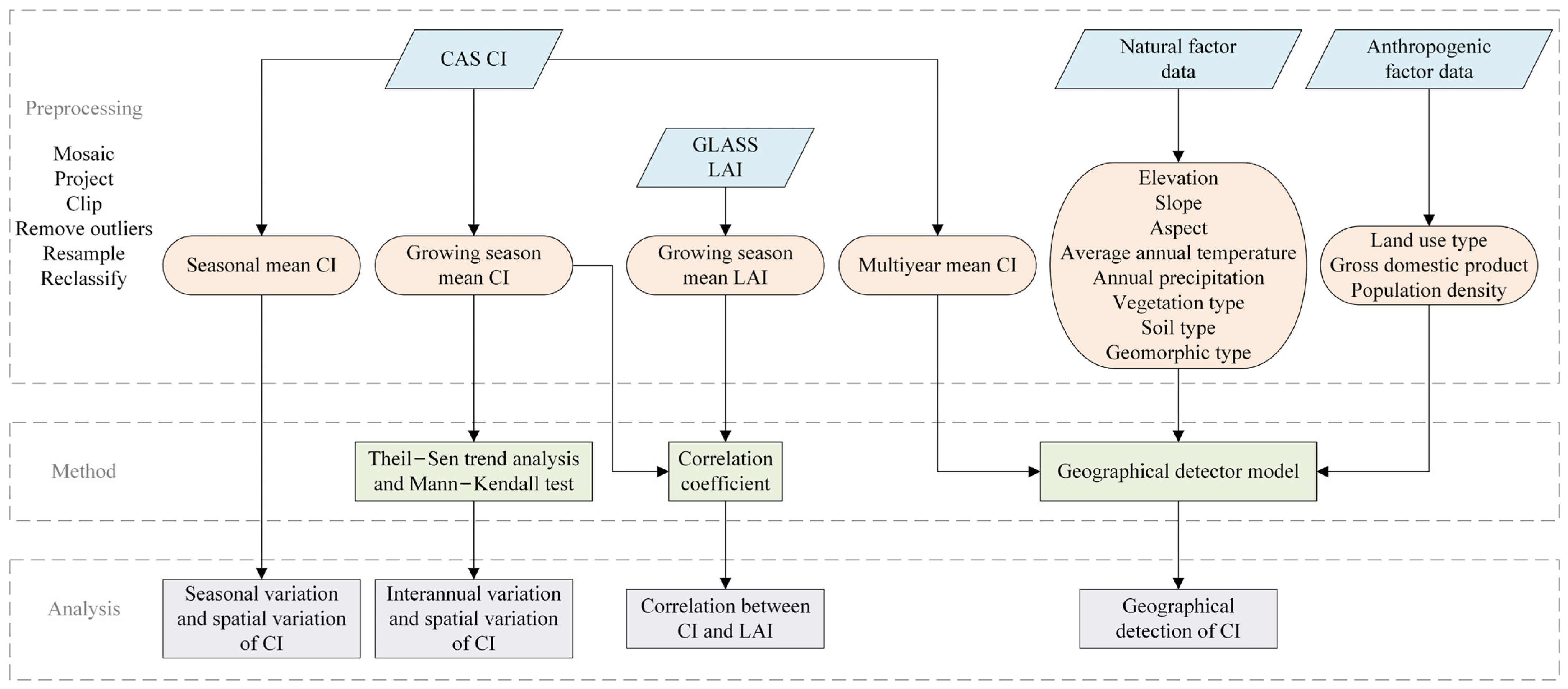
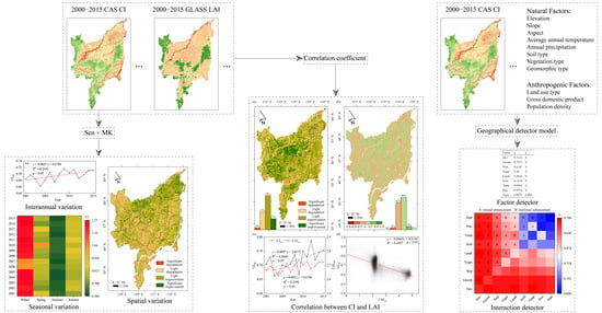
The framework of this study is given in Figure 2, including three modules: preprocessing, method, and analysis. The details of each method are introduced in Section 2.3.1, Section 2.3.2, Section 2.3.3, Section 2.3.4 and Section 2.3.5.

2.3.1. Theil–Sen Trend Analysis

Linear regression trend analysis has been widely used to understand vegetation dynamics [48]; however, it is sensitive to outliers or missing data [49]. Theil−Sen trend analysis, first proposed by Sen et al. [50], is also known as Sen’s slope. It is a non-parametric statistical method, which is robust for calculating the variation trend of a time series, and it is not sensitive to abnormal data [30]. The computational formula used to calculate Sen’s slope is shown below:
β = M e d i a n ( CI j CI i j i ) ,   i   <   j
where β indicates the variation trend of the CI times series data from 2000 to 2015; β < 0 indicates that CI exhibits a downward trend, and β > 0 indicates an upward trend. Median is a function used to calculate the median of a data set. CIj refers to the jth year CI data, and CIi is the CI data in year i.

2.3.2. Mann−Kendall Test

The Mann−Kendall test, which shows the insensitivity to outliers, is a non-parametric statistical test. Theil−Sen trend analysis is often combined with Mann−Kendall testing, which has been increasingly used to investigate the variation trend and test the statistical significance of a long time series data [51,52]. The Mann−Kendall test was originally proposed by Mann [53] and enhanced by Kendall and Sneyers [54]. Moreover, the samples of the long time series data do not need to follow a normal distribution or a linear variation trend. The equation is as follows:
Z = { S 1 v a r ( S ) , S   >   1 0 , S = 0 S + 1 v a r ( S ) , S   <   0
S = i = 1 n 1 j = i + 1 n s i g n ( CI j CI i )
s i g n ( CI j CI i ) = { 1 ,   CI j CI i   >   0 0 ,   CI j CI i = 0 1 ,   CI j CI i   <   0
v a r ( S ) = n ( n 1 ) ( 2 n + 5 ) i = 1 m t i ( t i 1 ) ( 2 t i + 5 ) 18
where Z denotes the standard normal test statistic; S is the test statistic; var is the variance function; n is the length of the time series; sign denotes the symbolic function; CIj and CIi are the CI data in year j and i, respectively; m refers to the datasets that repeat during the study period; and ti refers to the datasets that recur in group i. In this study, α was defined as 0.05, and |Z| > Z1−α/2 indicates the significant variation trend of CI time series.
Here, we used a combination of the above two methods to analyse the spatial and temporal variation characteristics of foliage CI in the Sanjiang Plain from 2001 to 2015 based on MATLAB software. Based on criteria in previous literature [55] and the actual features of the study area, areas with β < 0 and |Z| > 1.96 were classified as significantly degraded areas, areas with β > 0 and |Z| > 1.96 were classified as significantly improved areas, areas with β < 0 and |Z| ≤ 1.96 were classified as lightly degraded areas, and areas with β > 0 and |Z| ≤ 1.96 were classified as the lightly improved areas.

2.3.3. Correlation Coefficient

The correlation between two variables was often analysed using Pearson’s correlation coefficient. In this study, Pearson’s correlation analysis was performed to explore the correlation between CI and LAI at the pixel scale. The correlation coefficient can be found using the following formula:
R = i = 1 n ( LAI i LAI ¯ ) ( CI i CI ¯ ) i = 1 n ( LAI i LAI ¯ ) 2 ( CI i CI ¯ ) 2
where R ranges from −1 to 1, and the bigger the |R| value is, the higher the degree of correlation is between LAI and CI. LAIi and CIi are the LAI and CI in the year i, respectively; LAI ¯ and CI ¯ are the mean values of LAI and CI during the study period, respectively. Furthermore, n refers to the length of the study period. R > 0 indicates that the variation trends of LAI and CI are the same, R = 0 indicates that LAI and CI have no relationship, and R < 0 indicates that the variation trends of LAI and CI are inversely related [56].

2.3.4. Geographical Detector Model

The geographical detector model, proposed by Wang et al. [25], was first applied to explore the driving mechanism of environmental risks and human health in the Heshun Region of China. GDM is based on spatial variance analysis with no linear assumptions. It is a novel spatial statistical method used to explore the driving forces behind spatial differentiation [26]. GDM not only can quantify the influences of different driving factors on the spatial differentiation of the CI, but it can also ascertain the interactions between different driving forces [57]. Furthermore, when using GDM, the explanatory variable can be numerical data or qualitative data. The core concept behind GDM is that the spatial distribution of a response variable will be similar to its driving factors [58]. In other words, if some driving factors affect the spatial differentiation of the CI, then the spatial distribution of the CI and the driving factors may show greater consistency. The power of determinant (q) is used to measure the spatial correspondence or similarity between CI and driving forces, which can be expressed as
q = 1 i = 1 L N i σ i 2 N σ 2
where L denotes the total strata number of the driving factors; Ni and N denote the sample number in stratum i and the total sample number, respectively; and σi2 and σ2 refer to the local variance of CI within stratum i and the global variance of CI, respectively. The range of q is [0, 1]; thus, q = 0 indicates that the spatial distribution of CI is not affected by the driving forces, and q = 1 indicates that the driving forces completely determine the spatial characteristics of CI. The larger the value of q, the higher the spatial correlation between CI and driving factors.
GDM, which can mitigate the inherent limitations of the statistical methods [59], primarily involves four detectors: factor, risk, ecological, and interaction. Therefore, GDM has been increasingly used to explore the driving mechanism behind spatial differentiation. http://www.geodetector.cn/ accessed on 11 May 2021 is the Geodetector website, where more details regarding GDM can be found, along with the free software.
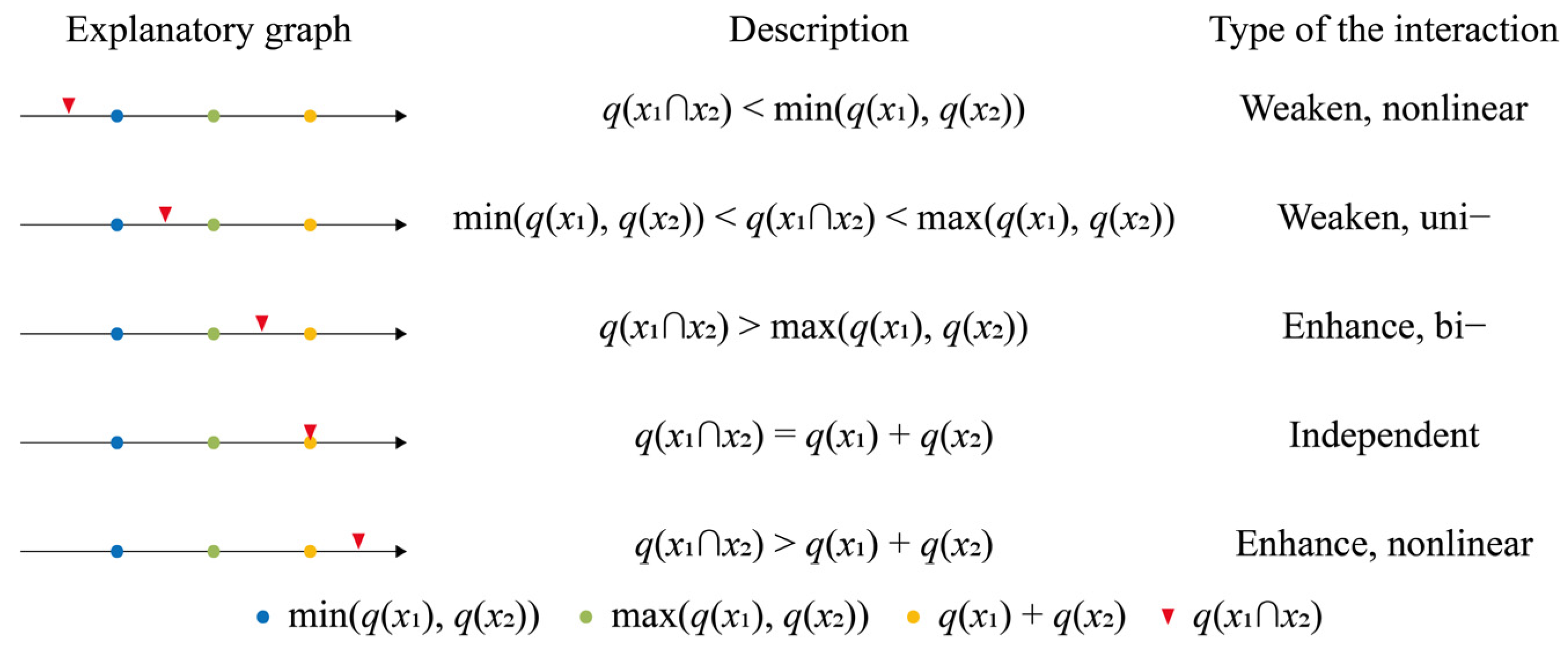
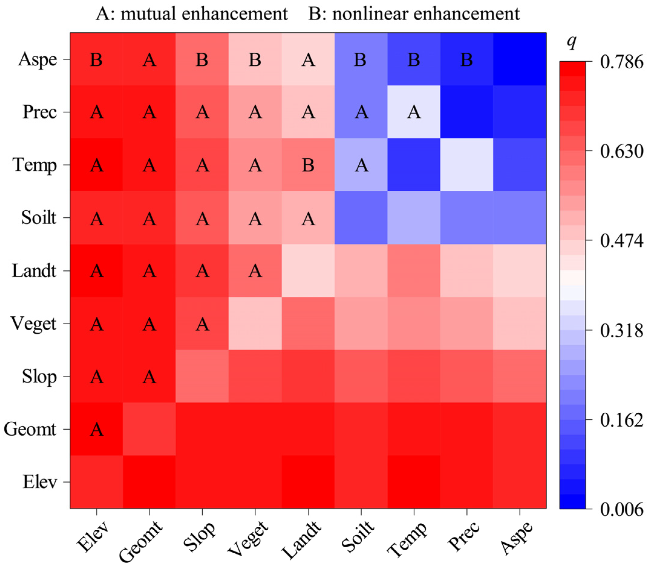
The factor detector assesses the explanatory power of each driving factor for the spatial differentiation of CI based on calculating the q value. A risk detector can determine the favourable ranges or characteristics of the driving factors to the foliage clumping effects with a confidence of 95%. The difference in the influences of two driving forces on the spatial differentiation of CI was ascertained using the ecological detector. The interactions between two driving forces were determined by the interaction detector. The q value of the two interactive factors was compared with that of a single factor; thus, the types of interactions can be divided into five classes (Figure 3).

2.3.5. Selection and Classification of Driving Factors

Owing to the comprehensive impacts of natural and anthropogenic factors, CI shows spatial characteristics in the Sanjiang Plain. In this study, we considered the main driving factors which have an important influence on the spatial differentiation of CI based on previous studies and the vegetation coverage in the Sanjiang Plain. Eight natural factors—the vegetation type (Veget), soil type (Soilt), geomorphic type (Geomt), average annual temperature (Temp), annual precipitation (Prec), elevation (Elev), slope (Slop), and aspect (Aspe)—and three anthropogenic factors—the land use type (Landt), gross domestic product (GDP), and population density (POP)—were selected as the driving factors. The spatial resolutions and the data sources of the CAS CI, natural factor data, and anthropogenic factor data differed. Therefore, this study took the GDM’s computing power and accuracy into consideration, resampling the resolution to 1 km based on the nearest neighbour method [60]. Moreover, all of the data were uniformly projected as Albers equal area conic projections.
When GDM is applied to analyse the driving mechanism, all of the driving factors must be qualitative data. Therefore, the numerical driving factors must be discretized into several strata. Discretization methods, such as the standard deviation, natural breaks, equal interval, geometrical interval, and quantile methods, are often used to discretize the numerical data. Natural breaks [61] were proposed to divide the numerical data into different intervals, with the minimum variance within intervals and the maximum variance between intervals. In this study, the natural breaks method was applied to reclassify the elevation, slope, average annual temperature, annual precipitation, population density, and gross domestic product into six classes. The aspect was reclassified into eight classes according to the eight geographical directions. The vegetation type, land use type, geomorphic type, and soil type were reclassified into seven, five, five, and six classes, respectively, according to their major types.

3. Results

3.1. Spatial and Temporal Variations of Land Use Type in the Sanjiang Plain from 2000 to 2015

3.1.1. Temporal Variations

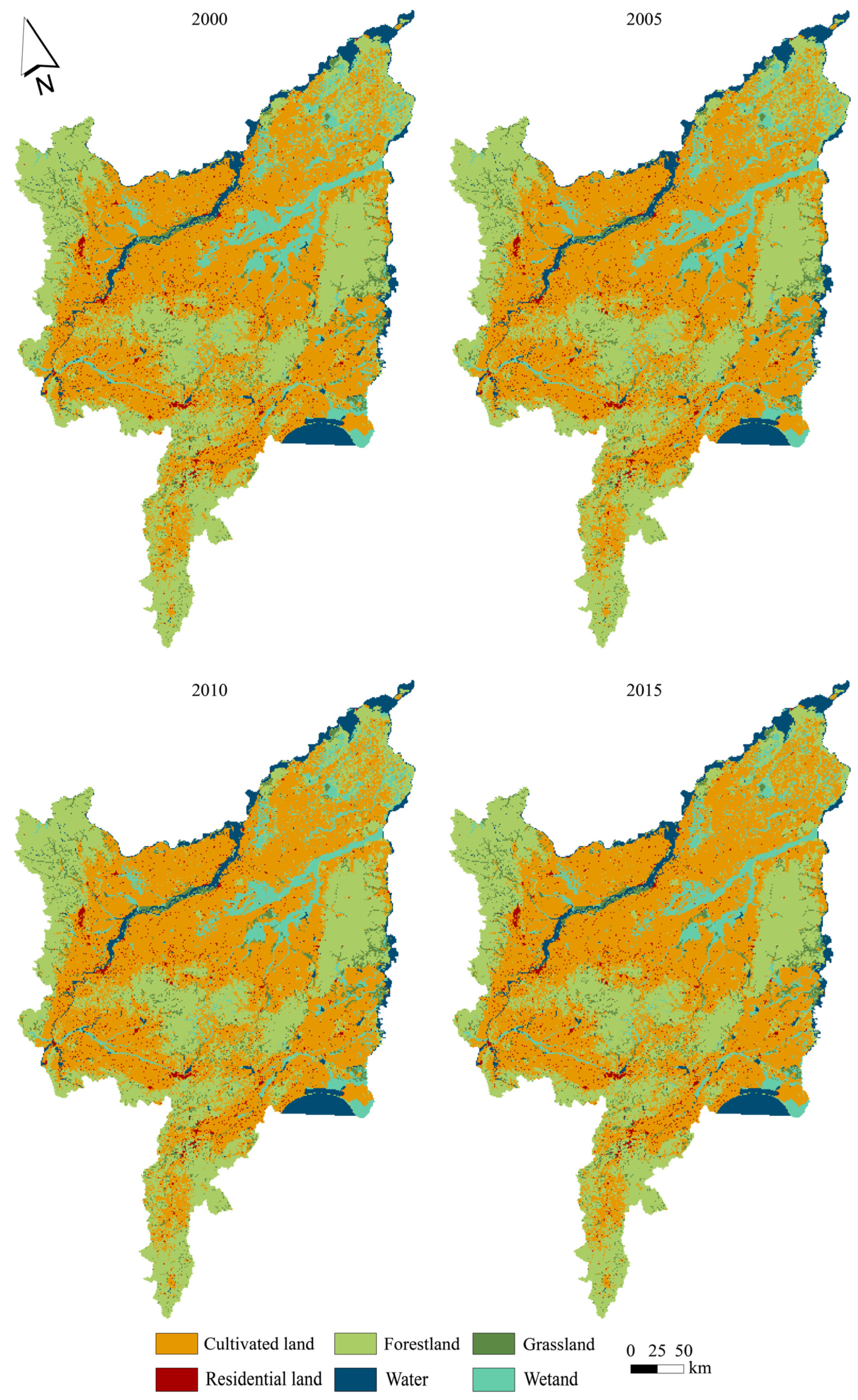
According to the main features of the land cover in the Sanjiang Plain and the Level 1 type of land use in Current Land Use Classification (http://www.gov.cn/ accessed on 11 May 2021), there were six kinds of land use types: cultivated land, water, grassland, forestland, residential land, and wetland. The cultivated land area in the Sanjiang Plain increased by 0.25 × 10⁴ km2 from 2000 to 2015, and its area proportion increased from 48.29% in 2000 to 50.61% in 2015 (Table 2). However, both the forestland area and the wetland area exhibit decreasing trends. The area proportion of the forestland decreased by 0.95% from 2000 to 2015, which represents a decrease of 0.10 × 10⁴ km2. The wetland area decreased by 0.15 × 10⁴ km2 from 2000 to 2015, and the area proportion of wetland areas decreased from 8.07% in 2000 to 6.70% in 2015. Grassland, water, and residential land exhibited stable variations, with small fluctuations in the area proportion (<0.05%).

3.1.2. Spatial Variations

The entire study area exhibited relative stability in terms of land use type (Figure 4), and the cultivated land area increased gradually, while the forestland area and wetland area decreased gradually. The northeastern and central regions of the study area were the major areas with decreased wetland, and the area with a larger reduction in forestland was mainly located in the northeastern region (Figure 5). The main spatial variations of land use type were the transformations from wetland to cultivated land and from forestland to cultivated land; the corresponding areas were 0.14 × 10⁴ km2 and 0.11 × 10⁴ km2, respectively (Table 3). Therefore, exploiting forestland and wetland were the primary methods to develop cultivated land, and cultivated land area increased greatly in the northeastern and central parts of the Sanjiang Plain from 2000 to 2015. Moreover, areas with grassland, water, and residential areas exhibited no obvious variations.

3.2. Spatial and Temporal Variations of CI in the Sanjiang Plain from 2000 to 2015

3.2.1. Interannual Variations

In this study, we used the growing season mean CI (CIGS) to assess the interannual variation of foliage CI in the Sanjiang Plain from 2001 to 2015. The mean value of CI in the growing season approximately ranged between 0.662 and 0.717, and the slope during the study period was 0.021∙10 a−1, which indicated that the overall interannual variation exhibited a slight upward trend. The overall CIGS value exhibited a decreasing trend from 2001 and 2004 and then increased from 2004 to 2006. Subsequently, the CIGS value decreased again in 2006−2007 and continued to fluctuate slightly after 2007 (Figure 6a). The area proportions of the variation trend of CIGS in the Sanjiang Plain from 2001 to 2015 are shown in Figure 6b. A total of 46.40% of the study area exhibited a downward trend, with a corresponding area of 4.80 × 10⁴ km2. The area of the region with an upward trend accounted for 53.60% of the study area and was 5.54 × 10⁴ km2. Lightly improved and lightly degraded areas exhibited the primary variation trends of CIGS in the Sanjiang Plain from 2001 to 2015, whose area proportions were 46.18% and 42.25%, respectively.

3.2.2. Seasonal Variations

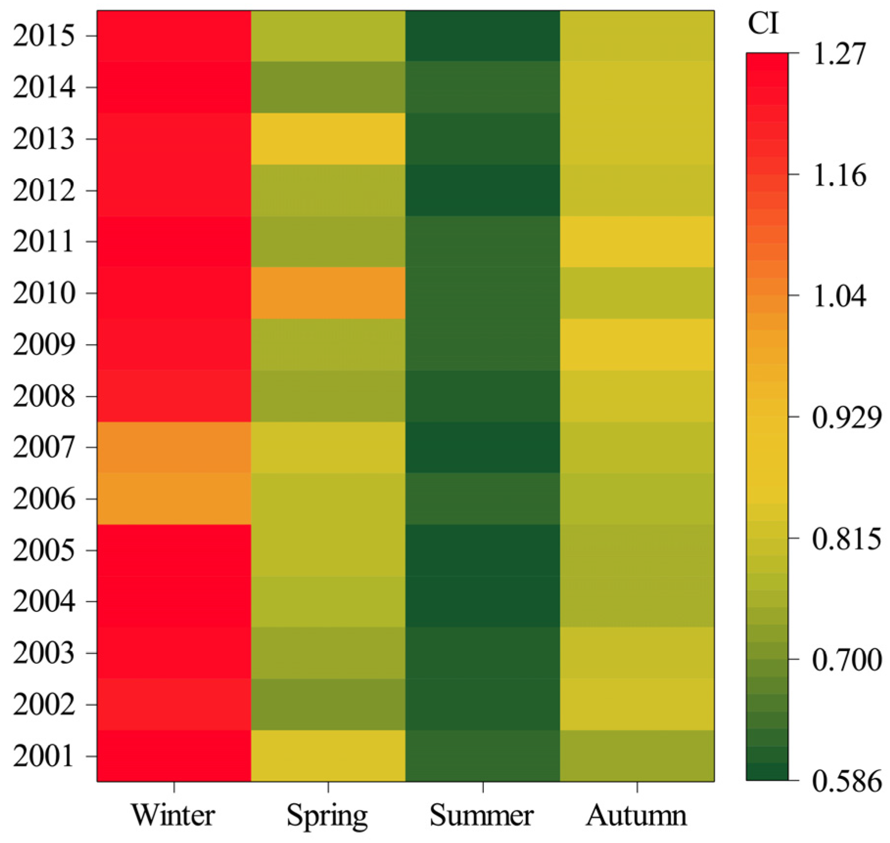
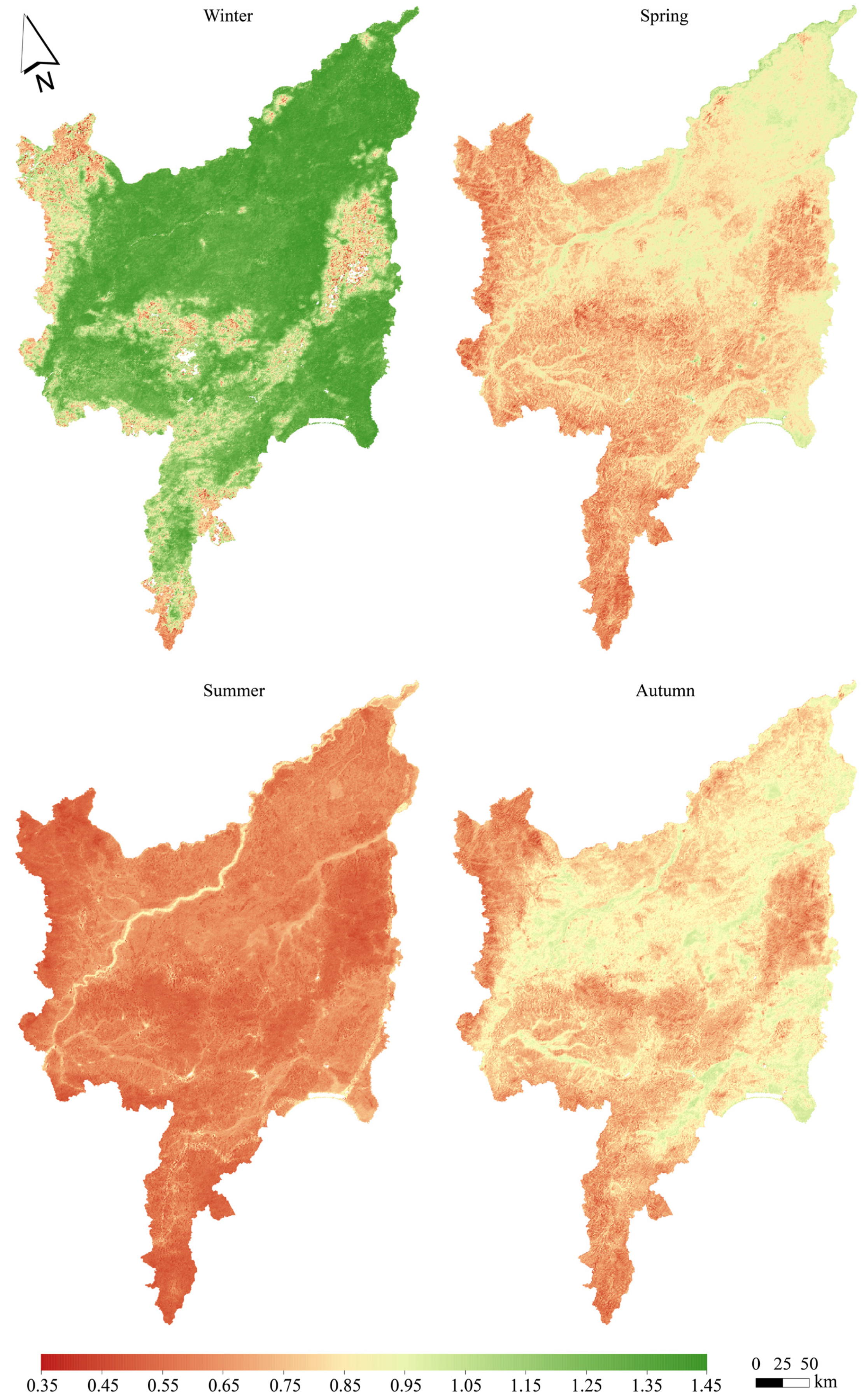
The seasonal mean CI in the Sanjiang Plain from 2001 to 2015 was obtained by the mean of a composition method, including the spring mean CI (CISP), summer mean CI (CISU), autumn mean CI (CIAU), and winter mean CI (CIWI). Figure 7 shows that the seasonal variation of CI was obvious throughout the study period. The overall CISU was the smallest value in the whole year, while the overall CIWI was the largest value in the whole year. In spring, the vegetation begins to grow, and foliage gradually becomes denser; therefore, the clumping effects are strengthened, and the CI value decreases gradually. The clumping effects in summer are the most obvious, and the multiyear mean CISU was 0.614. In autumn, the foliage begins to fall off and the clumping effects decrease gradually; thus, the CI value increases with time. In winter, the foliage is sparser than that in other seasons, and the multiyear mean CIWI was 1.206.

3.2.3. Spatial Variations

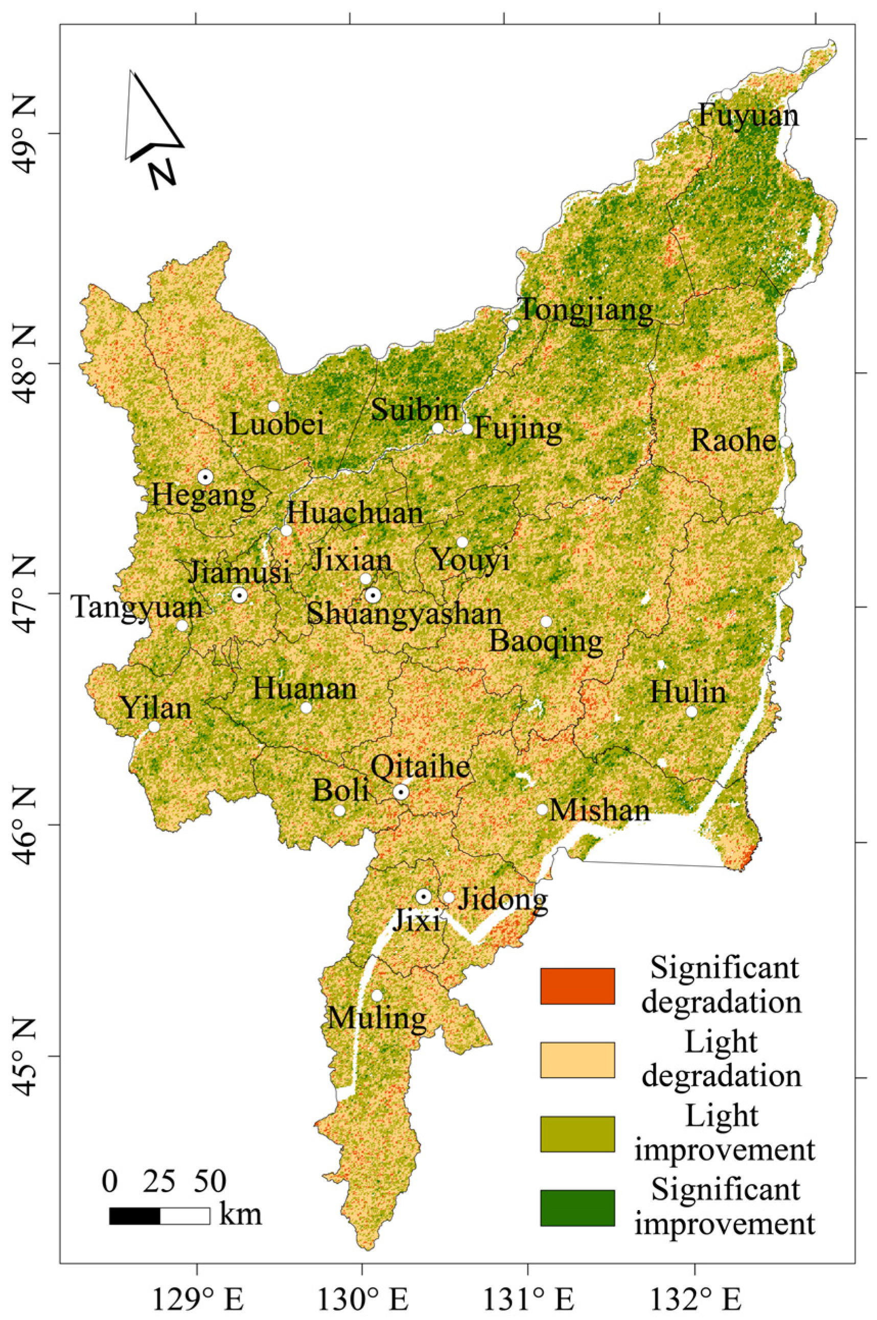
A slight overall variation of the clumping effects in the Sanjiang Plain during the study period was found, and the total area proportion of the areas with slight variations (light improvement and light degradation) was 88.43%. Most of the significantly improved areas were distributed in Fuyuan County, Tongjiang City, Suibin County, and eastern Luobei County. Areas with significant degradation were mainly distributed in northwestern Luobei County, northwestern Hegang City, Qitaihe City, west Mishan City, Jidong County, Jixi City, and Muling City (Figure 8).
The multiyear mean CI of each season was calculated by compositing a mean CI map for each season over fifteen years based on the mean composition method. The spatial distribution of the multiyear mean CI of each season was related to the spatial distribution of land use type (Figure 9). The main land use types in the Sanjiang Plain are cultivated land and forestland. In 2015, for example, 50.61% and 32.10% of the study area were occupied by cultivated land and forestland, respectively. Most of the cultivated land areas were distributed in the northern study area, and areas with forestland were mainly located in the southern, central, eastern, and northwestern regions of the study area. The multiyear mean CI of each season for cultivated land was greater than that for forestland; in other words, the clumping effects of the woody plants were more significant than those of herbaceous plants. Moreover, the multiyear mean CI values of cultivated land and forestland reached their maximum values in winter and decreased gradually in spring. The clumping effects of cultivated land and forestland in summer were the most intensive, and foliage later became sparse in autumn.
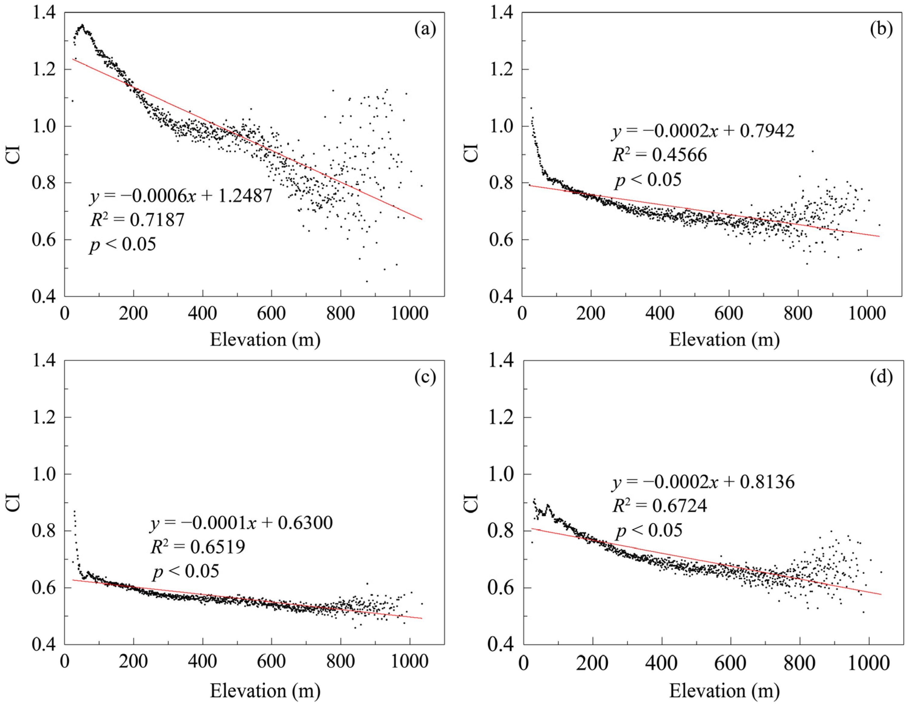
The CI variation trend with elevation in each season was explored based on the pixel-level statistics of the seasonal multiyear mean CI and elevation. As shown in Figure 10, the multiyear mean CI of each season exhibited a slight downward trend with elevation. The variation range of the multiyear mean CI in winter was the largest, while that of the multiyear mean CI in summer was the smallest. As the elevation increased by 100 m, the multiyear mean CI in winter and summer decreased by 0.06 and 0.01, respectively.

3.3. Correlation between CI and LAI in the Sanjiang Plain

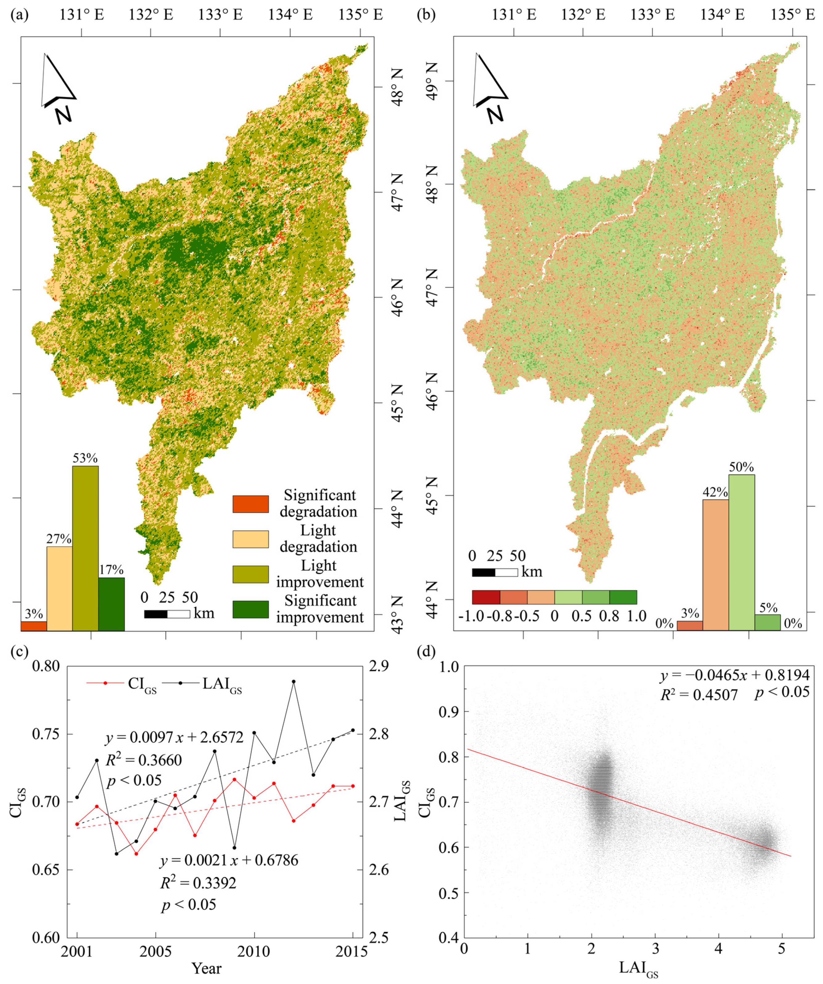
In this study, we used the growing season mean CI (CIGS) and growing season mean LAI (LAIGS) to analyse the correlation between CI and LAI in the Sanjiang Plain from 2001 to 2015. Figure 11c shows that both the CIGS and LAIGS exhibited slight upward trends, and their low growth rates were 0.021∙10 a−1 (p < 0.05) and 0.097∙10 a−1 (p < 0.05), respectively. The spatial distribution of the variation trend of LAIGS revealed an overall slight variation in LAI in the Sanjiang Plain during the study period, and areas with slight variations (light improvement and light degradation) occupied 80% of the total study area (Figure 11a). As described in Section 3.2.3, areas with slight variations (light improvement and light degradation) in CIGS occupied 88.43% of the total study area. Therefore, CIGS and LAIGS exhibited relative stability from 2001 to 2015.
The correlation coefficient of CIGS and LAIGS was calculated based on their time series over fifteen years, as shown in Figure 11b. Areas with positive correlation and negative correlation were 55% and 45% of the study area, respectively. However, only 7% of the study area was occupied by pixels with a significant correlation. Thus, temporally, the correlation between CIGS and LAIGS time series was not significant in the Sanjiang Plain from 2001 to 2015. Moreover, the multiyear mean CIGS and multiyear mean LAIGS were obtained using the mean composition method, and pixel-level statistical analysis showed that CIGS was negatively correlated with LAIGS in space. The two concentrated areas of scattered points in Figure 11d represent cultivated land and forestland, respectively. In other words, the LAI of cultivated land was larger than that of forestland, but the clumping effects of forestland were more intensive than those for cultivated land.

3.4. Geographical Detection of the Spatial Differentiation of CI in the Sanjiang Plain

3.4.1. Detection of the Significant Driving Factors for the Spatial Differentiation of CI

As mentioned in Section 2.3.5, eight natural factors and three anthropogenic factors were selected to analyse the driving factors for the spatial differentiation of CI in the Sanjiang Plain. Here, we first identified the driving factors that had a significant influence on the spatial differentiation of CI based on the factor detector. As shown in Table 4, the gross domestic product and population density had little influence on the spatial differentiation of CI and did not pass the significance test (p > 0.05). Therefore, the vegetation type (Veget), soil type (Soilt), geomorphic type (Geomt), average annual temperature (Temp), annual precipitation (Prec), elevation (Elev), slope (Slop), aspect (Aspe), and land use type (Landt) were used to investigate the driving mechanism of CI.

3.4.2. Detection of the Single Factors

The factor detector of GDM was applied to investigate the impact of each driving factor on the CI by calculating the q value. The higher the q value, the stronger the spatial association between the CI and division factors. In this study, we defined the driving factors with q values greater than 50% as the dominant driving factors, and driving factors with q values greater than 10% as the secondary driving factors. Natural factors and anthropogenic factors were ranked in descending order according to the magnitude of their impacts on the spatial distribution of CI: Elev > Geomt > Slop > Veget > Landt > Soilt > Temp > Prec > Aspe (first row in Table 5). All of the driving factors passed the significance test (p < 0.05).
The q values of the elevation, geomorphic type, and slope were the largest (0.7122, 0.7073, and 0.6102, respectively) and accounted for more than 50% of the spatial distribution of CI. Therefore, the dominant factors affecting CI were elevation, geomorphic type, and slope. Furthermore, the secondary driving forces of CI were vegetation type (0.4800), land use type (0.4664), and soil type (0.1818), all of which accounted for more than 10% of the spatial distribution of the CI. The q values of average annual temperature, annual precipitation, and aspect were below 10%, indicating that they had only a slight impact on the spatial differentiation of CI. However, the factor detector only revealed the impact of a single factor on CI based on the q value; thus, some driving factors might have a significant influence when interacting with others.

3.4.3. Detection of the Interactions among Factors

The interaction detector was applied to ascertain whether there was an interaction among two driving factors and to determine whether these interactions were weakened or enhanced by calculating the interactive q value. As shown in Figure 12, interactions between pairs of driving factors would enhance their impacts on the CI, and the types of interactions among driving factors included mutual enhancement and nonlinear enhancement. The q values of the interactions between the dominant driving factors and others were the largest; thus, topographic factors (elevation and slope) and geomorphic type dominated the spatial distribution of the CI.
The top five interactive q values were as follows, in descending order: Elev ∩ Geomt (0.7855) > Elev ∩ Landt (0.7697) > Elev ∩ Temp (0.7696) > Geomt ∩ Landt (0.7568) > Elev ∩ Prec (0.7548), indicating that interactions between elevation, geomorphic type, land use type, and climatic factors (average annual temperature and annual precipitation) had the greatest influence on CI. It is important to note that the q values of climatic factors were small (0.0949 and 0.0554), but the q values associated with the interactions between them and the elevation reached 0.7696 and 0.7548. Therefore, climatic factors also had a notable influence on the spatial differentiation of CI when they interacted with other driving factors. Moreover, nonlinear enhancement mainly occurred in the interactions between the aspect and other driving factors; therefore, the aspect also had an important influence on the spatial distribution of CI, and this impact also manifested in the interactions with other driving factors.

3.4.4. Detection of the Factor Ranges/Types Suitable for Clumping Effects of Foliage

The risk detector was applied to determine the optimal range/type of the driving factors for foliage clumping effects, with a confidence of 95%. The factor ranges/types with the smallest mean values of CIGS were most suitable for the clumping effects of foliage. The relationships between the spatial differentiation of CI and different driving forces differed (Table 6). Only relationships between CIGS and elevation, slope, and annual precipitation were monotonic; thus, the mean value of CIGS increased with them. The most optimal ranges of elevation, slope, and annual precipitation for the clumping effects of foliage were 589–1035 m, 5.8–13°, and 638.7–725.7 mm, respectively. Therefore, areas with high elevation, steep terrain, and abundant precipitation were more likely to be conducive to the clumping effects of foliage.
Moreover, the relationships between other driving factors and CIGS were non-monotonic. The mean values of CIGS decreased first and then increased with increasing average annual temperature, and the minimum mean value of CIGS appeared when the average annual temperature was 0.9–2.1 °C. In terms of the aspect, the mean value of CIGS reached 0.852 in the north. The geomorphic type with the smallest mean value of CIGS (0.648) was the moderate relief mountain; among all vegetation types, the mean value of CIGS of the coniferous and broad-leaved mixed forest was the smallest. For land use type and soil type, the minimum mean values of CIGS were found for forestland and leached soil, reaching 0.746 and 0.808, respectively.

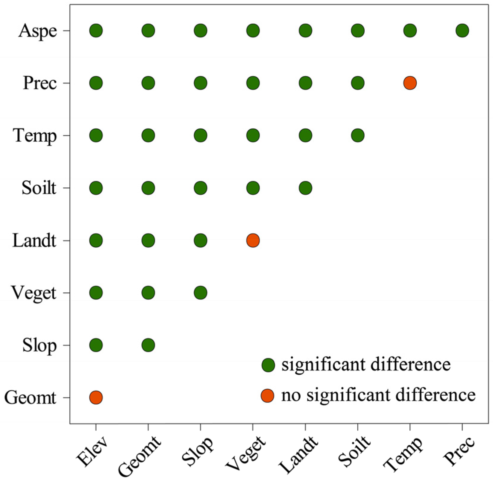
3.4.5. Detection of the Significant Differences between Factors

In terms of the impacts on CI, the presence of significant differences between driving forces was detected by the ecological detector in GDM, with a confidence of 95%. In Figure 13, the green circles denote that the two driving factors had a significant difference, and the red circles denote that the two driving factors had no significant difference. For dominant driving factors, there was no significant difference between elevation and geomorphic type, with corresponding q values of 0.7122 and 0.7073, respectively. Furthermore, for secondary driving factors, vegetation type and land use type exhibited similarities in terms of their influence on CI. The average annual temperature (0.0949) and annual precipitation (0.0554) had similar q values; thus, the difference between them was not significant. Furthermore, the statistical significance of the other driving factors indicated that they significantly differed.

4. Discussion

Previous studies have often used NDVI to investigate the spatio-temporal variations of regional vegetation. However, NDVI tends to become saturated during the flourishing period of vegetation growth and is affected by background soil disturbance [62]. Furthermore, CI is a significant parameter in the simulation of the interaction between the ecosystem and atmosphere. In this study, the spatial and temporal variation characteristics of CI in the Sanjiang Plain from 2001 to 2015 were analysed to provide a novel perspective for investigating variations in vegetation based on the CI and provide reliable foliage clumping effects for the retrieval of other vegetation structures and the simulation of land surface models. Furthermore, the effects of natural and anthropogenic forces on the spatial differentiation of CI were quantitatively explored to provide theoretical support for understanding the driving mechanism between CI and driving factors. However, the climatic factors, topographic factors, and anthropogenic factors that influenced the spatial distribution of CI were not fully considered. Although the time series of 15 years could indicate the relationships between CI and its driving factors to a certain extent, an even longer time series should be used to investigate the driving mechanism of the spatial differentiation of CI. Moreover, the spatio-temporal variations of CI for different vegetation types were not investigated.

4.1. Spatio-Temporal Variations of CI

Temporally, the overall interannual variation of CI in the Sanjiang Plain from 2001 to 2015 exhibited a slight upward trend with a slow growth rate of 0.021∙10 a−1 (p < 0.05). However, the seasonal variation was obvious, with the strongest clumping effects in the summer and the weakest clumping effects in the winter. Zhu [63] investigated the temporal characteristics of CI for major vegetation types in China from 2000 to 2013, finding that the mean values of CI in the growing season for all vegetation types exhibited relative stability, and the seasonal variation of CI was significant. The results in this study were relatively consistent with the abovementioned conclusions. Areas with significant improvement for CIGS in the Sanjiang Plain were mainly distributed in plain areas, with flat terrains and gentle slopes, and the variation of land use type was mainly from forestland to cultivated land. Therefore, CIGS showed a significant upward trend. Most areas with significant degradation were located in hills and small relief mountains that had gentle slopes, with elevations greater than 200 m, and the major land use type was forestland. Thus, the increase of clumping effects in the Sanjiang Plain could be related to improvements in vegetation growth.
The spatial distribution of the multiyear mean CI in each season was related to the spatial distribution of the land use type; this finding was consistent with the conclusion reached by Huang et al. [64] in the Daxing’an Mountains, Northeast China. Moreover, the multiyear mean CI of each season exhibited a slight downward trend with increasing elevation; the reason for this is that the main land use types of the plain with elevations less than 200 m and greater than 200 m were cultivated land and forestland, respectively. Thus, the overall multiyear mean CI in each season decreased with increasing elevation.

4.2. Driving Factors of the Spatial Distribution of CI

At present, to the best of our knowledge, there is no consistent conclusion on the correlation between CI and LAI. Based on field measurements, Fang et al. [21] believed that the CI of paddy rice was negatively correlated with LAI, while Qu et al. [65] found that the CI of deciduous coniferous forest was positively correlated with LAI. However, the pixel-level statistical analysis conducted herein indicated that CIGS was negatively correlated with LAIGS in space, and the correlation between their time series was not significant.
Furthermore, previous studies have shown that the main climatic factor that dominated the vegetation growth in the Sanjiang Plain was precipitation [37]. However, we found that topographic factors (elevation and slope) and geomorphic type dominated the vegetation growth in the Sanjiang Plain, thus dominating the spatial differentiation of CI. Topographic factors (elevation and slope), which were of great importance in redistributing the solar energy and precipitation [30], generally controlled the soil condition through different processes [66], determining the spatial characteristics of CI. Notably, climatic factors (average annual temperature and annual precipitation) and aspect had the smallest q values, but they still had a notable impact on the spatial differentiation of CI when they interacted with other driving factors. Related studies have also shown that the interactions between two driving forces could enhance the impact of a single factor [30,59,66]. Therefore, the government should use the land rationally according to the characteristics of topographic factors (elevation and slope) and geomorphic type in the Sanjiang Plain to improve grain production and ensure regional ecological security.

5. Conclusions

CAS CI products from 2001 to 2015 were used to analyse the spatial and temporal variation characteristics of CI in the Sanjiang Plain. Furthermore, the correlation between CI and LAI was explored based on the CAS CI and GLASS LAI products from 2001 to 2015. In addition, two climatic datasets (average annual temperature and annual precipitation) from 2001 to 2015, soil type data, vegetation type data, three topographic data sets (aspect, slope, and elevation), geomorphic type data, and land use type data were used to quantify the driving forces of the spatial distribution of CI. The major conclusions drawn are as follows:
(1) In terms of temporal variations, the interannual variation of CI in the Sanjiang Plain from 2001 to 2015 was not obvious, and the overall variation exhibited a slight upward trend, with a slow growth rate of 0.021∙10 a−1 (p < 0.05). However, the seasonal variation was obvious, with the strongest clumping effects in summer and the weakest clumping effects in winter.
(2) In terms of spatial variations, lightly improved and lightly degraded areas were the main variation trends of CIGS in the Sanjiang Plain from 2001 to 2015, with area proportions of 46.18% and 42.25%, respectively. The spatial distribution of the multiyear mean CI of each season was related to the spatial distribution of the land use type, and the multiyear mean CI in each season exhibited a slight downward trend with increasing elevation. Moreover, the multiyear mean CI of each season for cultivated land was greater than that for forestland.
(3) Temporally, the correlation between the CI time series and LAI time series was not significant in the Sanjiang Plain from 2001 to 2015. Spatially, CI exhibited a negative correlation with LAI.
(4) The elevation, geomorphic type, and slope were the main factors dominating the spatial differentiation of CI. Furthermore, the vegetation type, land use type, and soil type were the secondary driving forces of the spatial distribution of CI. Notably, as single driving factors, climatic factors (average annual temperature and annual precipitation) and aspect had the smallest q values but still had a notable impact on the spatial differentiation of CI when they interacted with other driving factors. Furthermore, each driving factor had the optimal range/type for foliage clumping effects.

Author Contributions

The authors’ contributions to this article are as follows: conceptualization, Z.Z.; methodology, K.H.; software, K.H. and Z.G.; validation, Z.Z.; formal analysis, K.H. and Z.Z.; investigation, Z.Z. and Y.L.; resources, K.H.; data curation, K.H. and Z.G.; writing—original draft preparation, K.H., Z.Z., and H.F.; writing—review and editing, K.H., Z.Z., and H.F.; visualization, K.H.; supervision, Z.Z.; project administration, M.G.; funding acquisition, Z.Z. All authors have read and agreed to the published version of the manuscript.

Funding

This research was funded by the National Natural Science Foundation of China (Grant No.42071085), Open Project of the State Key Laboratory of Cryospheric Science (Grant No. SKLCS 2020−10), and the National Natural Science Foundation of China (Grant No.41701087).

Data Availability Statement

Not applicable.

Acknowledgments

The authors would like to thank the National Earth System Science Data Center, National Science & Technology Infrastructure of China (http://www.geodata.cn/ accessed on 11 May 2021) for the CAS (Chinese Academy of Sciences) CI products and the GLASS (Global LAnd Surface Satellite) LAI products, the United States Geological Survey (https://earthexplorer.usgs.gov/ accessed on 11 May 2021) for the SRTM data, and the Resource and Environment Science and Data Center (http://www.resdc.cn/ accessed on 11 May 2021) for the other natural factor data and anthropogenic factor data.

Conflicts of Interest

The authors declare no conflict of interest.

References

  1. Nilson, T. A theoretical analysis of the frequency of gaps in plant stands. Agric. Meteorol. 1971, 8, 25–38. [Google Scholar] [CrossRef]
  2. Chen, J.M.; Black, T.A. Foliage area and architecture of plant canopies from sunfleck size distributions. Agric. For. Meteorol. 1992, 60, 249–266. [Google Scholar] [CrossRef]
  3. Chen, J.M.; Rich, P.M.; Gower, S.T.; Norman, J.M.; Plummer, S. Leaf area index of boreal forests: Theory, techniques, and measurements. J. Geophys. Res. 1997, 102, 29429–29443. [Google Scholar] [CrossRef]
  4. Chianucci, F.; Cutini, A. Estimation of canopy properties in deciduous forests with digital hemispherical and cover photography. Agric. For. Meteorol. 2013, 168, 130–139. [Google Scholar] [CrossRef]
  5. Zou, J.; Zhuang, Y.; Chianucci, F.; Mai, C.; Lin, W.; Leng, P.; Luo, S.; Yan, B. Comparison of seven inversion models for estimating plant and woody area indices of leaf–on and leaf–off forest canopy using explicit 3D forest scenes. Remote Sens. 2018, 10, 1297. [Google Scholar] [CrossRef] [Green Version]
  6. Macfarlane, C.; Hoffman, M.; Eamus, D.; Kerp, N.; Higginson, S.; McMurtrie, R.; Adams, M. Estimation of leaf area index in eucalypt forest using digital photography. Agric. For. Meteorol. 2007, 143, 176–188. [Google Scholar] [CrossRef]
  7. Chen, B.; Liu, J.; Chen, J.M.; Croft, H.; Gonsamo, A.; He, L.; Luo, X. Assessment of foliage clumping effects on evapotranspiration estimates in forested ecosystems. Agric. For. Meteorol. 2016, 216, 82–92. [Google Scholar] [CrossRef]
  8. Chen, J.M.; Mo, G.; Pisek, J.; Liu, J.; Deng, F.; Ishizawa, M.; Chan, D. Effects of foliage clumping on the estimation of global terrestrial gross primary productivity. Glob. Biogeochem. Cycles 2012, 26, GB1019. [Google Scholar] [CrossRef]
  9. Baldocchi, D.D.; Wilson, K.B.; Gu, L. How the environment, canopy structure and canopy physiological functioning influence carbon, water and energy fluxes of a temperate broad-leaved deciduous forest—An assessment with the biophysical model CANOAK. Tree Physiol. 2002, 22, 1065–1077. [Google Scholar] [CrossRef] [Green Version]
  10. Chen, Q.; Baldocchi, D.; Gong, P.; Dawson, T. Modeling radiation and photosynthesis of a heterogeneous savanna woodland landscape with a hierarchy of model complexities. Agric. For. Meteorol. 2008, 148, 1005–1020. [Google Scholar] [CrossRef]
  11. Baldocchi, D.D.; Wilson, K.B. Modeling CO2 and water vapor exchange of a temperate broadleaved forest across hourly to decadal time scales. Ecol. Modell. 2001, 142, 155–184. [Google Scholar] [CrossRef]
  12. Chen, J.M.; Liu, J.; Leblanc, S.G.; Lacaze, R.; Roujean, J.-L. Multi-angular optical remote sensing for assessing vegetation structure and carbon absorption. Remote Sens. Environ. 2003, 84, 516–525. [Google Scholar] [CrossRef]
  13. Wang, Y.; Woodcock, C.; Buermann, W.; Stenberg, P.; Voipio, P.; Smolander, H.; Häme, T.; Tian, Y.; Hu, J.; Knyazikhin, Y.; et al. Evaluation of the MODIS LAI algorithm at a coniferous forest site in Finland. Remote Sens. Environ. 2004, 91, 114–127. [Google Scholar] [CrossRef]
  14. Liu, R.; Chen, J.M.; Liu, J.; Deng, F.; Sun, R. Application of a new leaf area index algorithm to China’s landmass using MODIS data for carbon cycle research. J. Environ. Manag. 2007, 85, 649–658. [Google Scholar] [CrossRef]
  15. Pisek, J.; Chen, J.M.; Nilson, T. Estimation of vegetation clumping index using MODIS BRDF data. Int. J. Remote Sens. 2011, 32, 2645–2657. [Google Scholar] [CrossRef]
  16. Zhu, G.; Ju, W.; Chen, J.M.; Gong, P.; Xing, B.; Zhu, J. Foliage clumping index over China’s landmass retrieved from the MODIS BRDF parameters product. IEEE Trans. Geosci. Remote Sens. 2012, 50, 2122–2137. [Google Scholar] [CrossRef]
  17. Wei, S.; Fang, H. Estimation of canopy clumping index from MISR and MODIS sensors using the normalized difference hotspot and darkspot (NDHD) method: The influence of BRDF models and solar zenith angle. Remote Sens. Environ. 2016, 187, 476–491. [Google Scholar] [CrossRef]
  18. Wei, S.; Fang, H.; Schaaf, C.B.; He, L.; Chen, J.M. Global 500 m clumping index product derived from MODIS BRDF data (2001–2017). Remote Sens. Environ. 2019, 232, 111296. [Google Scholar] [CrossRef]
  19. Chianucci, F.; Zou, J.; Leng, P.; Zhuang, Y.; Ferrara, C. A new method to estimate clumping index integrating gap fraction averaging with the analysis of gap size distribution. Can. J. For. Res. 2019, 49, 471–479. [Google Scholar] [CrossRef]
  20. Pisek, J.; Lang, M.; Nilson, T.; Korhonen, L.; Karu, H. Comparison of methods for measuring gap size distribution and canopy nonrandomness at Järvselja RAMI (RAdiation transfer Model Intercomparison) test sites. Agric. For. Meteorol. 2011, 151, 365–377. [Google Scholar] [CrossRef]
  21. Fang, H.; Li, W.; Wei, S.; Jiang, C. Seasonal variation of leaf area index (LAI) over paddy rice fields in NE China: Intercomparison of destructive sampling, LAI–2200, digital hemispherical photography (DHP), and AccuPAR methods. Agric. For. Meteorol. 2014, 198–199, 126–141. [Google Scholar] [CrossRef]
  22. García, M.; Gajardo, J.; Riaño, D.; Zhao, K.; Martín, P.; Ustin, S. Canopy clumping appraisal using terrestrial and airborne laser scanning. Remote Sens. Environ. 2015, 161, 78–88. [Google Scholar] [CrossRef]
  23. Wei, S. Estimation of clumping index from multi–angle remote sensing data. Ph.D. Thesis, Chinese Academy of Sciences, Beijing, China, 2017. [Google Scholar]
  24. Zhu, L.; Meng, J.; Zhu, L. Applying Geodetector to disentangle the contributions of natural and anthropogenic factors to NDVI variations in the middle reaches of the Heihe River Basin. Ecol. Indic. 2020, 117, 106545. [Google Scholar] [CrossRef]
  25. Wang, J.; Li, X.; Christakos, G.; Liao, Y.; Zhang, T.; Gu, X.; Zheng, X. Geographical detectors–based health risk assessment and its application in the neural tube defects study of the Heshun Region, China. Int. J. Geogr. Inf. Sci. 2010, 24, 107–127. [Google Scholar] [CrossRef]
  26. Wang, J.; Xu, C. Geodetector: Principle and prospective. Acta Geogr. Sin. 2017, 72, 116–134. [Google Scholar]
  27. Huang, C.; Liu, K.; Zhou, L. Spatio–temporal trends and influencing factors of PM2.5 concentrations in urban agglomerations in China between 2000 and 2016. Environ. Sci. Pollut. Res. 2020, 28, 10988–11000. [Google Scholar] [CrossRef]
  28. Zhou, Y.; Li, X.; Tong, C.; Huang, H. The geographical pattern and differentiational mechanism of rural poverty in China. Acta Geogr. Sin. 2021, 76, 903–920. [Google Scholar]
  29. Du, Z.; Zhang, X.; Xu, X.; Zhang, H.; Wu, Z.; Pang, J. Quantifying influences of physiographic factors on temperate dryland vegetation, Northwest China. Sci. Rep. 2017, 7, 40092. [Google Scholar] [CrossRef]
  30. Meng, X.; Gao, X.; Li, S.; Lei, J. Spatial and temporal characteristics of vegetation NDVI changes and the driving forces in Mongolia during 1982–2015. Remote Sens. 2020, 12, 603. [Google Scholar] [CrossRef] [Green Version]
  31. Peng, W.; Kuang, T.; Tao, S. Quantifying influences of natural factors on vegetation NDVI changes based on geographical detector in Sichuan, western China. J. Clean. Prod. 2019, 233, 353–367. [Google Scholar] [CrossRef]
  32. Zhao, W.; Hu, Z.; Guo, Q.; Wu, G.; Chen, R.; Li, S. Contributions of climatic factors to interannual variability of the vegetation index in Northern China grasslands. J. Clim. 2019, 33, 175–183. [Google Scholar] [CrossRef]
  33. Meng, Q.; Wu, Z.; Du, Z.; Zhang, H. Quantitative influence of regional fractional vegetation cover based on geodetector model—Take the Beijing–Tianjin sand source region as an example. China Environ. Sci. 2021, 41, 826–836. [Google Scholar]
  34. Tao, S.; Kuang, T.; Peng, W.; Wang, G. Analyzing the spatio–temporal variation and drivers of NDVI in upper reaches of the Yangtze River from 2000 to 2015: A case study of Yibin City. Acta Ecol. Sin. 2020, 40, 5029–5043. [Google Scholar]
  35. Liu, J.; Zhao, D.; Tian, X.; Zhao, L.; Liu, J. Landscape pattern dynamics and driving forces analysis in the Sanjiang Plain from 1954 to 2010. Acta Ecol. Sin. 2014, 34, 3234–3244. [Google Scholar]
  36. Zhang, B.; Lu, C.; Sun, Q.; Xiao, W.; Hou, B.; Yan, L. Effects of climate and land use change on vegetation coverage in Sanjiang Plain. Water Res. Power 2017, 35, 18–22. [Google Scholar]
  37. Zhang, J.; Zhang, B.; Ma, B.; Cao, B.; Liang, J.; Ma, S. Spatial–temporal variation of NDVI in Sanjiang Plain and its response to climate change. J. Des. Res. 2019, 39, 206–213. [Google Scholar]
  38. Yang, L.; Shen, F.; Zhang, L.; Cai, Y.; Yi, F.; Zhou, C. Quantifying influences of natural and anthropogenic factors on vegetation changes using structural equation modeling: A case study in Jiangsu Province, China. J. Clean. Prod. 2021, 280, 124330. [Google Scholar] [CrossRef]
  39. Li, H.; Zheng, L.; Lei, Y.; Li, C.; Zhou, K. Comparison of NDVI and EVI based on EOS/MODIS data. Prog. Geogr. 2007, 26, 26–32. [Google Scholar]
  40. Yan, F.; Zhang, S.; Liu, X.; Chen, D.; Chen, J.; Bu, K.; Yang, J.; Chang, L. The effects of spatiotemporal changes in land degradation on ecosystem services values in Sanjiang Plain, China. Remote Sens. 2016, 8, 917. [Google Scholar] [CrossRef] [Green Version]
  41. Liu, T.; Yu, L.; Bu, K.; Yan, F.; Zhang, S. Seasonal local temperature responses to paddy field expansion from rain–fed farmland in the cold and humid Sanjiang Plain of China. Remote Sens. 2018, 10, 2009. [Google Scholar] [CrossRef] [Green Version]
  42. Wang, H.; Song, C. Regional ecological risk assessment of wetlands in the Sanjiang Plain. Prog. Geogr. 2019, 38, 872–882. [Google Scholar]
  43. Xiao, Z.; Liang, S.; Wang, J.; Chen, P.; Yin, X.; Zhang, L.; Song, J. Use of general regression neural networks for generating the GLASS leaf area index product from time–series MODIS surface reflectance. IEEE Trans. Geosci. Remote Sens. 2014, 52, 209–223. [Google Scholar] [CrossRef]
  44. Xiao, Z.; Liang, S.; Wang, J.; Xiang, Y.; Zhao, X.; Song, J. Long-time-series global land surface satellite leaf area index product derived from MODIS and AVHRR surface reflectance. IEEE Trans. Geosci. Remote Sens. 2016, 54, 5301–5318. [Google Scholar] [CrossRef]
  45. Farr, T.G.; Rosen, P.A.; Caro, E.; Crippen, R.; Duren, R.; Hensley, S.; Kobrick, M.; Paller, M.; Rodriguez, E.; Roth, L.; et al. The shuttle radar topography mission. Rev. Geophys. 2007, 45, RG2004. [Google Scholar] [CrossRef] [Green Version]
  46. Xu, X. Spatial Distribution Data Set of GDP in China. Data Registration and Publication System of Chinese Academy of Sciences. 2017. Available online: https://www.resdc.cn/data.aspx?DATAID=252 (accessed on 11 May 2021).
  47. Xu, X. Spatial Distribution Data Set of Population in China. Data Registration and Publication System of Chinese Academy of Sciences. 2017. Available online: https://www.resdc.cn/data.aspx?DATAID=251 (accessed on 11 May 2021).
  48. Stow, D.; Daeschner, S.; Hope, A.; Douglas, D.; Petersen, A.; Myneni, R.; Zhou, L.; Oechel, W. Variability of the seasonally integrated normalized difference vegetation index across the north slope of Alaska in the 1990s. Int. J. Remote Sens. 2003, 24, 1111–1117. [Google Scholar] [CrossRef]
  49. Neeti, N.; Eastman, J.R. A contextual Mann–Kendall approach for the assessment of trend significance in image time series. Trans. GIS 2011, 15, 599–611. [Google Scholar] [CrossRef]
  50. Sen, P.K. Estimates of the regression coefficient based on Kendall’s Tau. J. Am. Stat. Assoc. 1968, 63, 1379–1389. [Google Scholar] [CrossRef]
  51. Li, S.; Yang, S.; Liu, X.; Liu, Y.; Shi, M. NDVI-based analysis on the influence of climate change and human activities on vegetation restoration in the Shaanxi–Gansu–Ningxia Region, Central China. Remote Sens. 2015, 7, 11163–11182. [Google Scholar] [CrossRef] [Green Version]
  52. Zhao, W.; Li, J.; Chu, L.; Wang, T.; Li, Z.; Cai, C. Analysis of spatial and temporal variations in vegetation index and its driving force in Hubei Province in the last 10 years. Acta Ecol. Sin. 2019, 39, 7722–7736. [Google Scholar]
  53. Mann, H.B. Non-parametric tests against trend. Econ. J. Econ. Soc. 1945, 13, 245–259. [Google Scholar]
  54. Forthofer, R.N.; Lehnen, R.G. Rank correlation methods. In Public Program Analysis: A New Categorical Data Approach; Forthofer, R.N., Lehnen, R.G., Eds.; Springer: Boston, MA, USA, 1981; pp. 146–163. [Google Scholar]
  55. Zhang, W.; Jin, H.; Shao, H.; Li, A.; Li, S.; Fan, W. Temporal and spatial variations in the leaf area index and its response to topography in the Three–River Source Region, China from 2000 to 2017. ISPRS Int. J. Geo Inf. 2021, 10, 33. [Google Scholar] [CrossRef]
  56. Guo, J.; Hu, Y.; Xiong, Z.; Yan, X.; Ren, B.; Bu, R. Spatiotemporal variations of growing–season NDVI associated with climate change in Northeastern China’s permafrost zone. Pol. J. Environ. Stud. 2017, 26, 1521–1529. [Google Scholar] [CrossRef]
  57. Wang, Z.; Liang, L.; Sun, Z.; Wang, X. Spatiotemporal differentiation and the factors influencing urbanization and ecological environment synergistic effects within the Beijing–Tianjin–Hebei urban agglomeration. J. Environ. Manag. 2019, 243, 227–239. [Google Scholar] [CrossRef]
  58. Wang, J.F.; Hu, Y. Environmental health risk detection with GeogDetector. Environ. Model. Softw. 2012, 33, 114–115. [Google Scholar] [CrossRef]
  59. Chen, T.; Xia, J.; Zou, L.; Hong, S. Quantifying the influences of natural factors and human activities on NDVI changes in the Hanjiang River Basin, China. Remote Sens. 2020, 12, 3780. [Google Scholar] [CrossRef]
  60. Wang, W.; Samat, A.; Abuduwaili, J. Geo–detector based spatio–temporal variation characteristics and driving factors analysis of NDVI in Central Asia. Remote Sens. Land Res. 2019, 31, 32–40. [Google Scholar]
  61. Jenks, G.F. The data model concept in statistical mapping. Inter. Year. Carto. 1967, 7, 186–190. [Google Scholar]
  62. Wu, D.; Ma, Y.; Wu, H.; Xiao, Y.; Li, H. Characteristics of temporal and spatial evolution and driving forces of vegetation index in Sichuan based on MODIS–EVI. Res. Soil Water Conserv. 2020, 27, 230–236, 243. [Google Scholar]
  63. Zhu, G. Spatial-temporal characteristics of foliage clumping index in China during 2000–2013. Chin. Sci. Bull. 2016, 61, 1595–1603. [Google Scholar] [CrossRef] [Green Version]
  64. Huang, T.; Fan, W.; Mao, X.; Yu, Y. Foliage clumping index of main vegetation types in Daxing’an Mountains, Northeast China. Chin. J. of Appl. Ecol. 2017, 28, 757–762. [Google Scholar]
  65. Qu, Y. MLAOS: A multi–point linear array of optical sensors for coniferous foliage clumping index measurement. Sensors 2014, 14, 9271–9289. [Google Scholar] [CrossRef] [PubMed] [Green Version]
  66. Zhang, Y.; Hu, Q.; Zou, F. Spatio-temporal changes of vegetation net primary productivity and its driving factors on the Qinghai–Tibetan Plateau from 2001 to 2017. Remote Sens. 2021, 13, 1566. [Google Scholar] [CrossRef]
Figure 1. Study area.
Remotesensing 13 02797 g001
Figure 2. Flowchart of this study.
Remotesensing 13 02797 g002
Figure 3. Types of Interactions.
Remotesensing 13 02797 g003
Figure 4. Spatial distribution of land use type.
Remotesensing 13 02797 g004
Figure 5. Spatial variation of land use type.
Remotesensing 13 02797 g005
Figure 6. Interannual variations of growing season mean CI (CIGS): (a) point plot of CIGS and (b) area proportions of the variation trend of CIGS.
Remotesensing 13 02797 g006
Figure 7. Seasonal variation of CI.
Remotesensing 13 02797 g007
Figure 8. Spatial variation of CIGS.
Remotesensing 13 02797 g008
Figure 9. Spatial distribution of the multiyear mean CI for each season.
Remotesensing 13 02797 g009
Figure 10. Variation trend of CI with elevation in each season: (a) winter; (b) spring; (c) summer; and (d) autumn.
Remotesensing 13 02797 g010
Figure 11. Correlation between CI and LAI: (a) spatial distribution of the variation trend of growing season mean LAI (LAIGS); (b) spatial distribution of the correlation coefficient between CIGS and LAIGS; (c) point plot of CIGS and LAIGS; and (d) statistical analysis of multiyear mean CIGS and multiyear mean LAIGS.
Remotesensing 13 02797 g011
Figure 12. Interactions between driving factors.
Remotesensing 13 02797 g012
Figure 13. Statistical significance of driving factors.
Remotesensing 13 02797 g013
Table 1. Driving factors.
Factor TypesAbbreviationsFactorsSources
Natural factorsElevElevationUSGS (https://earthexplorer.usgs.gov/ accessed on 11 May 2021)
SlopSlopeDerived from SRTM DEM
AspeAspect
TempAverage annual temperatureResource and Environment Science and Data Center, RESDC (http://www.resdc.cn/ accessed on 11 May 2021)
PrecAnnual precipitation
VegetVegetation type
SoiltSoil type
GeomtGeomorphic type
Anthropogenic factorsLandtLand use typeRESDC (http://www.resdc.cn/ accessed on 11 May 2021)
GDPGross domestic product
POPDensity of population
Table 2. Temporal variation of land use type.
YearCultivated Land (%)Forestland (%)Grassland (%)Water (%)Residential Land (%)Wetland (%)
200048.2933.053.894.781.928.07
200548.6432.963.994.821.927.67
201049.2732.663.954.831.927.37
201550.6132.103.854.821.926.70
Table 3. Transfer matrix of land use type. (Unit: km2).
2015Cultivated LandForestland Grassland Residential LandWater Wetland Aggregate
2000
Cultivated land51,95615510076111652,314
Forestland114734,5776454835,805
Grassland193283941128244215
Residential land75212001002079
Water29010515145185
Wetland1430157032572008743
Aggregate54,83034,7774177208652197252108,341
Table 4. Detection of the significant driving factors for the spatial differentiation of CI.
FactorElevGeomtSlopVegetLandtSoiltTempPrecAspeGDPPOP
q0.71180.70710.60960.47930.46570.18120.09430.05490.00770.00470.0015
p0.0000.0000.0000.0000.0000.0000.0000.0000.0071.0001.000
Table 5. The q value of each driving factor.
FactorElevGeomtSlopVegetLandtSoiltTempPrecAspe
q0.71220.70730.61020.48000.46640.18180.09490.05540.0079
p0.0000.0000.0000.0000.0000.0000.0000.0000.006
Table 6. The optimal range/type for clumping effects of foliage.
FactorOptimal Range/TypeMean Value of CIGS
Elev (m)589–10350.643
GeomtModerate relief mountain0.648
Slop (°)5.8–130.670
VegetConiferous and broad-leaved mixed forest0.682
LandtForestland0.746
SoiltLeached soil0.808
Temp (°C)0.9–2.10.818
Prec (mm)638.7–725.70.822
Aspe (°)0–22.5, 337.5–3600.852
Publisher’s Note: MDPI stays neutral with regard to jurisdictional claims in published maps and institutional affiliations.