
True-Color Reconstruction Based on Hyperspectral LiDAR Echo Energy


Abstract
:1. Introduction
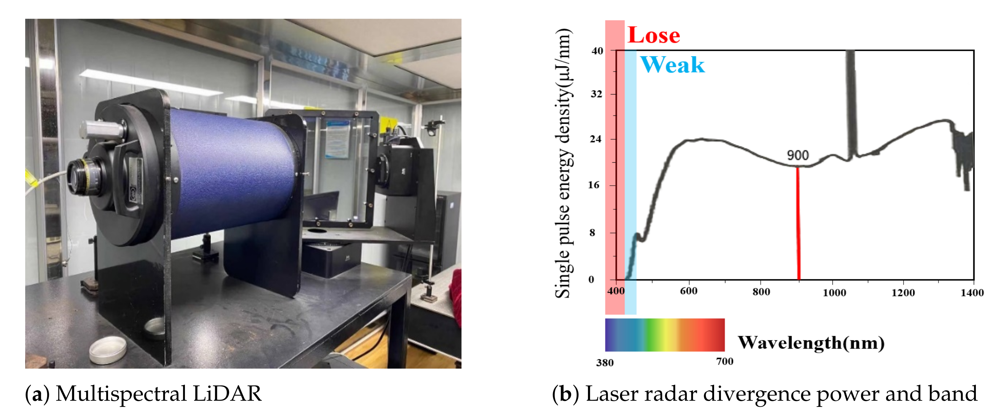
2. HSL System Description
3. Hyperbolic Tangent Normalization and Correction Model with Parameters
4. Improved Spectrum Reconstruction of Gradient Boosting Decision Tree Series Forecasting
5. Results and Discussion
5.1. Results
5.2. Discussion
6. Conclusions
Author Contributions
Funding
Institutional Review Board Statement
Informed Consent Statement
Data Availability Statement
Conflicts of Interest
GitHub
References
- Beger, R.; Gedrange, C.; Hecht, R.; Neubert, M. Data fusion of extremely high resolution aerial imagery and LiDAR data for automated railroad centre line reconstruction. ISPRS J. Photogramm. Remote Sens. 2011, 66, S40–S51. [Google Scholar] [CrossRef]
- Debes, C.; Merentitis, A.; Heremans, R.; Hahn, J.; Frangiadakis, N.; van Kasteren, T.; Liao, W.; Bellens, R.; Pižurica, A.; Gautama, S.; et al. Hyperspectral and LiDAR data fusion: Outcome of the 2013 GRSS data fusion contest. IEEE J. Sel. Top. Appl. Earth Obs. Remote Sens. 2014, 7, 2405–2418. [Google Scholar] [CrossRef]
- Khodadadzadeh, M.; Li, J.; Prasad, S.; Plaza, A. Fusion of hyperspectral and LiDAR remote sensing data using multiple feature learning. IEEE J. Sel. Top. Appl. Earth Obs. Remote Sens. 2015, 8, 2971–2983. [Google Scholar] [CrossRef]
- Dong, J.; Zhuang, D.; Huang, Y.; Fu, J. Advances in multi-sensor data fusion: Algorithms and applications. Sensors 2009, 9, 7771–7784. [Google Scholar] [CrossRef] [PubMed] [Green Version]
- Alonzo, M.; Bookhagen, B.; Roberts, D.A. Urban tree species mapping using hyperspectral and lidar data fusion. Remote Sens. Environ. 2014, 148, 70–83. [Google Scholar] [CrossRef]
- Dalponte, M.; Bruzzone, L.; Gianelle, D. Tree species classification in the Southern Alps based on the fusion of very high geometrical resolution multispectral/hyperspectral images and LiDAR data. Remote Sens. Environ. 2012, 123, 258–270. [Google Scholar] [CrossRef]
- Sankey, T.; Donager, J.; McVay, J.; Sankey, J.B. UAV lidar and hyperspectral fusion for forest monitoring in the southwestern USA. Remote Sens. Environ. 2017, 195, 30–43. [Google Scholar] [CrossRef]
- Gong, W.; Sun, J.; Shi, S.; Yang, J.; Du, L.; Zhu, B.; Song, S. Investigating the potential of using the spatial and spectral information of multispectral LiDAR for object classification. Sensors 2015, 15, 21989–22002. [Google Scholar] [CrossRef] [Green Version]
- Liu, Q.; Liu, Y.; Pointer, M.R.; Huang, Z.; Wu, X.; Chen, Z.; Luo, M.R. Color discrimination metric based on the neutrality of lighting and hue transposition quantification. Opt. Lett. 2020, 45, 6062–6065. [Google Scholar] [CrossRef]
- Liang, J.; Wan, X. Optimized method for spectral reflectance reconstruction from camera responses. Opt. Express 2017, 25, 28273–28287. [Google Scholar] [CrossRef]
- Technical Committee International Commission on Illumination. Practical Methods for the Measurement of Reflectance and Transmittance; Commission Internationale de l’Eclairage: Vienna, Austria, 1998. [Google Scholar]
- Liang, J.; Xiao, K.; Pointer, M.R.; Wan, X.; Li, C. Spectra estimation from raw camera responses based on adaptive local-weighted linear regression. Opt. Express 2019, 27, 5165–5180. [Google Scholar] [CrossRef] [PubMed] [Green Version]
- Gong, W.; Song, S.; Zhu, B.; Li, F.; Cheng, X. Multi-wavelength canopy LiDAR for remote sensing of vegetation: Design and system performance. ISPRS J. Photogramm. Remote Sens. 2012, 69, 1–9. [Google Scholar]
- Woodhouse, I.H.; Nichol, C.; Sinclair, P.; Jack, J.; Morsdorf, F.; Malthus, T.J.; Patenaude, G. A multispectral canopy LiDAR demonstrator project. IEEE Geosci. Remote Sens. Lett. 2011, 8, 839–843. [Google Scholar] [CrossRef]
- Gaulton, R.; Danson, F.; Ramirez, F.; Gunawan, O. The potential of dual-wavelength laser scanning for estimating vegetation moisture content. Remote Sens. Environ. 2013, 132, 32–39. [Google Scholar] [CrossRef]
- Song, S.; Wang, B.; Gong, W.; Chen, Z.; Lin, X.; Sun, J.; Shi, S. A new waveform decomposition method for multispectral LiDAR. ISPRS J. Photogramm. Remote Sens. 2019, 3, 40–49. [Google Scholar] [CrossRef]
- Sun, J.; Shi, S.; Yang, J.; Chen, B.; Gong, W.; Du, L.; Mao, F.; Song, S. Estimating leaf chlorophyll status using hyperspectral lidar measurements by PROSPECT model inversion. Remote Sens. Environ. 2018, 1, 1–7. [Google Scholar] [CrossRef]
- Zhao, X.; Shi, S.; Yang, J.; Gong, W.; Sun, J.; Chen, B.; Guo, K.; Chen, B. Active 3D imaging of vegetation based on multi-wavelength fluorescence LiDAR. Sensors 2020, 3, 935. [Google Scholar] [CrossRef] [PubMed] [Green Version]
- Chen, B.; Shi, S.; Sun, J. Using HSI Color Space to Improve the Multispectral Lidar Classification Error Caused by Measurement Geometry. IEEE Trans. Geosci. Remote Sens. 2020, 99, 1–13. [Google Scholar] [CrossRef]
- Wang, J.; Li, C. Development and prospect of hyperspectral imager and its application. Chin. J. Space Sci. 2021, 41, 22–33. (In Chinese) [Google Scholar]
- Wang, B.; Song, S.; Gong, W.; Cao, X.; He, D.; Chen, Z.; Lin, X.; Li, F.; Sun, J. Color Restoration for Full-Waveform Multispectral LiDAR Data. Remote Sens. 2020, 12, 593. [Google Scholar] [CrossRef] [Green Version]
- Chen, B.; Shi, S.; Gong, W.; Sun, J.; Chen, B.; Du, L.; Yang, J.; Guo, K.; Zhao, X. True-Color Three-Dimensional Imaging and Target Classification Based on Hyperspectral LiDAR. Remote Sens. 2019, 11, 1541. [Google Scholar] [CrossRef] [Green Version]
- Zhou, J.; Zeng, Y.; Wang, X.; Wu, C.; Cai, Z.; Gao, B.Z.; Gu, D.; Shao, Y. The capture of antibodies by antibody-binding proteins for ABO blood typing using SPR imaging-based sensing technology. Sens. Actuators B Chem. 2019, 304, 1–15. [Google Scholar] [CrossRef]
- Taulier, A.; Levillain, P.; Lemonnier, A. Determining methemoglobin in blood by zero-crossing-point first-derivative spectrophotometry. Clin. Chem. 2020, 33, 10–17. [Google Scholar] [CrossRef]
- Owega, S.; Poitras, D. Local similarity matching algorithm for determining SPR angle in surface plasmon resonance sensors. Sens. Actuators B Chem. 2007, 123, 35–41. [Google Scholar] [CrossRef]
- Wang, X.; Dong, L.; Zhan, S. Without-Baseline Centroid Algorithm for Surface Plasmon Resonance Spectra. Chin. J. Sens. Actuators 2012, 25, 365–369. [Google Scholar]
- Zhan, S.; Wang, X.; Liu, Y. Fast centroid algorithm for determining the surface plasmon resonance angle using the fixed-boundary method. Meas. Sci. Technol. 2011, 22, 1–7. [Google Scholar] [CrossRef]
- Adam, C.; Vivek, K. Denoising Hyperspectral Imagery and Recovering Junk Bands using Wavelets and Sparse Approximation. In Proceedings of the IEEE Geoscience and Remote Sensing Symposium, Denver, CO, USA, 31 July–4 August 2006; pp. 387–390. [Google Scholar]
- Zhong, P.; Wang, R. Multiple-Spectral-Band CRFs for Denoising Junk Bands of Hyperspectral Imagery. IEEE Trans. Geosci. Remote Sens. 2013, 51, 2260–2275. [Google Scholar] [CrossRef]
- Yin, J.; Sun, J.; Jia, X. Sparse Analysis Based on Generalized Gaussian Model for Spectrum Recovery with Compressed Sensing Theory. IEEE J. Sel. Top. Appl. Earth Obs. Remote Sens. 2015, 8, 2752–2759. [Google Scholar] [CrossRef]
- Liu, X.; Zhang, Y.; Teng, T.; Ding, Z. Estimation of Vegetation Water Content based on Bi-inverted Gaussian Fitting Spectral Feature Analysis Using Hyperspectral Data. Remote Sens. Technol. Appl. 2016, 31, 1075–1082. [Google Scholar]
- Arad, B.; Ben-Shahar, O. Sparse Recovery of Hyperspectral Signal from Natural RGB Images. In European Conference on Computer Vision; Springer: Berlin/Heidelberg, Germany, 2016; pp. 19–34. [Google Scholar]
- Schonlau, M. Boosted regression (boosting): An introductory tutorial and a Stata plugin. Stata J. 2005, 5, 330–354. [Google Scholar] [CrossRef]
- Arumugam, P.; Kuppan, V. A GBDT-SOA approach for the system modelling of optimal energy management in grid-connected micro-grid system. Int. J. Energy Res. 2020, 45, 1–19. [Google Scholar]
- Friedman, J.H. Greedy Function Approximation: A Gradient Boosting Machine. Ann. Stat. 2005, 29, 1189–1232. [Google Scholar]
- Zhang, J.; Xu, D.; Hao, K.; Zhang, Y.; Chen, W.; Liu, J.; Gao, R.; Wu, C.; De Marinis, Y. FS-GBDT: Identification multicancer-risk module via a feature selection algorithm by integrating Fisher score and GBDT. Brief. Bioinform. 2020, 1, 1–13. [Google Scholar] [CrossRef] [PubMed]
- Zhang, W.; Yu, J.; Zhao, A.; Zhou, X. Predictive model of cooling load for ice storage air-conditioning system by using GBDT. Energy Rep. 2021, 7, 1588–1597. [Google Scholar] [CrossRef]
- Chen, Y.; Liu, Y. Which Risk Factors Matter More for Psychological Distress during the COVID-19 Pandemic? An Application Approach of Gradient Boosting Decision Trees. Int. J. Environ. Res. Public Health 2021, 18, 1–17. [Google Scholar]
- Amiri, M.M.; Amirshahi, S.H. A step by step recovery of spectral data from colorimetric information. J. Opt. 2015, 44, 373–383. [Google Scholar] [CrossRef]
- Cao, B.; Liao, N.; Cheng, H. Spectral reflectance reconstruction from RGB images based on weighting smaller color difference group. Color Res. Appl. 2017, 42, 327–332. [Google Scholar] [CrossRef]


| Num | RMSE % Only the Reconstruction Part Is Calculated | |
|---|---|---|
| 1 | 6.148465671 | 1.76555 |
| 2 | 6.061711912 | 1.591006 |
| 3 | 6.555953527 | 2.924124 |
| 4 | 6.503468054 | 2.899935 |
| 5 | 6.331956111 | 2.120579 |
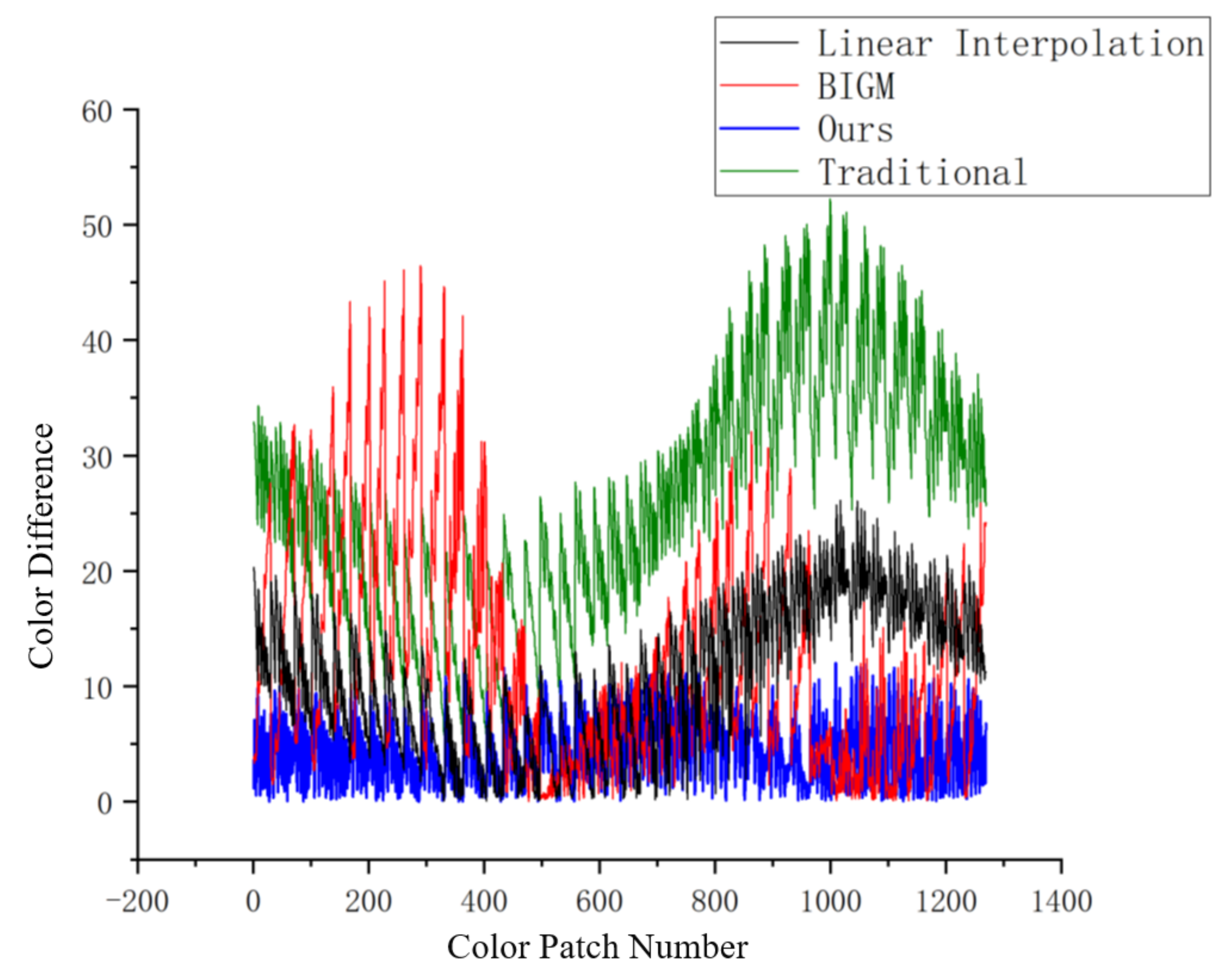
| Num | Algorithm | Result | Color Difference of 1269 Munsell Color Chip | X-Rite Color Checker |
|---|---|---|---|---|
| 1 | Missing | Mean | 26.42 | 26.009 |
| 400–700 nm | Max | 55.417 | 47.687 | |
| 2 | Algorithm | Mean | 4.67 | 6.484 |
| in this paper | Max | 13.22472 | 10.514766 | |
| 3 | Bi-inverted | Mean | 11.999 | 16.034 |
| Gaussian model | Max | 26.714542 | 22.414988 | |
| 4 | Linear | Mean | 11.052 | 13.28 |
| Interpolation | Max | 29.2666469 | 21.1400417 | |
| 5 | Gradient Boosting | Mean | 7.771 | 8.954 |
| Decision Tree | Max | 17.3334863 | 13.59832 |
Publisher’s Note: MDPI stays neutral with regard to jurisdictional claims in published maps and institutional affiliations. |
© 2021 by the authors. Licensee MDPI, Basel, Switzerland. This article is an open access article distributed under the terms and conditions of the Creative Commons Attribution (CC BY) license (https://creativecommons.org/licenses/by/4.0/).
Share and Cite
Wang, T.; Wan, X.; Chen, B.; Shi, S. True-Color Reconstruction Based on Hyperspectral LiDAR Echo Energy. Remote Sens. 2021, 13, 2854. https://doi.org/10.3390/rs13152854
Wang T, Wan X, Chen B, Shi S. True-Color Reconstruction Based on Hyperspectral LiDAR Echo Energy. Remote Sensing. 2021; 13(15):2854. https://doi.org/10.3390/rs13152854
Chicago/Turabian StyleWang, Tengfeng, Xiaoxia Wan, Bowen Chen, and Shuo Shi. 2021. "True-Color Reconstruction Based on Hyperspectral LiDAR Echo Energy" Remote Sensing 13, no. 15: 2854. https://doi.org/10.3390/rs13152854