Project Report

Sino–EU Earth Observation Data to Support the Monitoring and Management of Agricultural Resources

1
Institute of Methodologies for Environmental Analysis (IMAA)-National Council of Research (CNR), C. da S. Loja, 85050 Tito Scalo, Italy
2
Department of Agriculture, Forests, Nature and Energy (DAFNE), Università della Tuscia, via San Camillo de Lellis, 01100 Viterbo, Italy
3
School of Aerospace Engineering (SIA), University of Rome “La Sapienza”, SIA, via Salaria, 851, 00138 Roma, Italy
4
National Engineering Research Center for Information Technology in Agriculture, Beijing 100097, China
5
Key Laboratory of Digital Earth Science, Aerospace Information Research Institute, Chinese Academy of Sciences, Beijing 100094, China
6
European Space Agency, ESRIN, via Galileo Galilei 1, 00044 Frascati, Italy
7
Department of Computer Science, Maynooth University, W23 F2H6 Dublin, Ireland
*
Author to whom correspondence should be addressed.
Remote Sens. 2021, 13(15), 2889; https://doi.org/10.3390/rs13152889
Submission received: 21 May 2021 / Revised: 2 July 2021 / Accepted: 9 July 2021 / Published: 23 July 2021
(This article belongs to the Special Issue ESA - NRSCC Cooperation Dragon 4 Final Results)

Abstract

:
Novel approaches and algorithms to estimate crop physiological processes from Earth Observation (EO) data are essential to develop more sustainable management practices in agricultural systems. Within this context, this paper presents the results of different research activities carried out within the ESA-MOST Dragon 4 programme. The paper encompasses two research avenues: (a) the retrieval of biophysical variables of crops and yield prediction; and (b) food security related to different crop management strategies. Concerning the retrieval of variables, results show that LAI, derived by radiative transfer model (RTM) inversion, when assimilated into a crop growth model (i.e., SAFY) provides a way to assess yields with a higher accuracy with respect to open loop model runs: 1.14 t·ha−1 vs 4.42 t·ha−1 RMSE for assimilation and open loop, respectively. Concerning food security, results show that different pathogens could be detected by remote sensing satellite data. A k coefficient higher than 0.84 was achieved for yellow rust, thus assuring a monitoring accuracy, and for the diseased samples k was higher than 0.87. Concerning permanent crops, neural network (NN) algorithms allow classification of the Pseudomonas syringae pathogen on kiwi orchards with an overall accuracy higher than 91%.

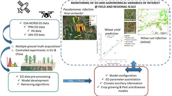
Graphical Abstract

1. Introduction

Currently, an extraordinary amount of medium and high spatial resolution remote sensing data can be obtained and applied for agricultural applications when combining European and Chinese satellite acquisitions [1,2,3,4,5,6]. This can produce a strong impact if a common targeting and operational policy is applied. In both European and Asian continents, agricultural system monitoring activities face very similar observational requirements, both in terms of satellite repetition frequencies and of spectral and spatial resolutions. At present, decametric satellite spatial resolution is the best available option to map and monitor crop biophysical parameters, crop yield, crop phenology and crop pests and disease in fragmented agricultural systems such as those of Southern Europe and China [7,8,9].
The European ESA Sentinels, the ESA Third Party Mission (TPM) and the Chinese satellites constellation, when used in synergy, provide a unique satellite data set that needs to be fully exploited for the benefit of the agricultural domain [10]. It is of great interest to the SINO-EU community to test new procedures and algorithms, as well as to improve the existing ones, to exploit the potential agronomic information that can be retrieved when assimilating the ensemble of the SINO-EU multi-temporal and multi-sensor satellite data sets.
Meanwhile, a full EO synergy between China and the EU will be envisaged for the community, and joint research in the framework of the ESA and Ministry of Science and Technology (MOST) collaborative program (http://dragon4.esa.int/, accessed on 13 April 2021) are planned to exploit and demonstrate the contribution of SINO-UE components to agricultural systems. The research included activities for: (a) methodological issues concerning the optimal algorithms to be applied for the quantitative assessment of crop vegetation variables and their errors and uncertainties related to the remote sensing observations; and (b) the methodological aspects related to the assimilation of EO-based vegetation quantitative variables within crop models as well as crop models’ formulation errors and parameter uncertainties.
This work aims at providing examples of the added value that a SINO-EU EO satellite data synergy could provide for specific agricultural variables’ retrieval and prediction. In this study, activities focused on common cropping systems in Italy and China for: (1) the estimation of variables of agronomic interest linked to the water and nitrogen cycling in the agro-ecosystems; (2) the improvement of the prediction of wheat yield and quality, both at the regional and the farm scale; and (3) the detection, recognition and mapping of the status related to biotic stresses for cereal crops (yellow rust and Fusarium) and orchards (attacked by Xylella fastidiosa or other diseases).
To fulfill these general objectives, a research roadmap has been drawn to identify the steps required to exploit the collected SINO-EU data sets.
The first step of this joint research was to retrieve crop biophysical variables, such as Leaf Area Index (LAI), leaf pigments both at the leaf and the canopy scales and the Fraction of Absorbed Photosynthetically Active Radiation (FAPAR), to understand their impact on a variety of agronomical applications including precision agriculture, crop traits monitoring and yield prediction as well as grain quality. To these aims, the team has co-authored a study [11] that evaluates the performance of the most recent retrieval algorithms, including hybrid methods as well as machine learning regression (MLR) algorithms exploring active learning strategies. The performance of different retrieval algorithms using Sentinel-2 data were tested on two test areas: Maccarese (Italy) and Sunshy (China). Results of study [11] showed that it is difficult to identify a single algorithm as the best for the retrieval of the biophysical crop variables considered in all cases. Nevertheless, the study showed that the estimation of the different variables was consistent for both the Italian and Chinese datasets.
The second step regards the use of the retrieved biophysical variables within crop growth models. Crop biophysical variables and indices derived from EO optical imagery have been used as a proxy for other crop characteristics that cannot be directly accessed from EO sensors, such as crop yield. However, as highlighted in the recent review by Weiss et al. [10], the link between optical EO and crop yield is rather complex and nonlinear, due to the interactions of many agro-environmental factors such as weather, plant growth and development dynamics, water and nutrient balance and crop management. Empirical methods that link, through parametric or nonparametric regression, crop optical properties to crop yield show poor generalization capability and require additional field work for calibration and validation, especially when applied on a new location or crop variety. Coupling crop models, which describe processes and interactions within the agricultural systems using mathematical equations, with EO data, which provide in-season updates of the canopy state, has been considered a winning strategy to obtain more accurate yield predictions [12]. Data assimilation, for example, is a procedure that updates a model state variable, such as for example simulated LAI, each time a new in-season observation, i.e., EO-derived LAI, is acquired, correcting the model simulation trajectories. The first assimilation tests, as part of the results obtained in the framework of the ESA-MOST Dragon 3 cooperation programme (https://dragon3.esa.int/web/dragon-3/home, accessed on April 13, 2021), were focused on the estimation of wheat yield, both at the field and the regional scales. The study of [11] assimilated LAI and canopy cover (CC) into the SAFY model [13] for the Yangling area (Central China) using both the Huan Jing (HJ) satellite HJ1A/B and Landsat 8 Operational Land Imager (OLI) imagery. In this first experiment, the retrieved LAI values were assimilated into the SAFY models by applying an Ensemble Kalman filter (EnKF), while the obtained CC values were used in the Particle Swarm Optimization (PSO) procedures in the Aquacrop model. The results of this study [14] showed that this assimilation approach could lead to an estimation error of about 20% for the yield. These results are also extremely dependent on models’ assimilation procedures (EnKF for SAFY and PSO for Aquacrop) and previous model calibration. In more recent tests, with different assimilation procedures, EO data proved to be useful in combination with the Aquacrop-OS crop model, allowing for more precise estimations of crop yield as a result of the sensitivity analysis and calibration of Aquacrop using EO-retrieved canopy cover [15,16]. A further step of this research regarded the prediction of both yield and grain quality in protein concentration before harvest by using hyperspectral and atmospheric data in a hierarchical linear modelling (HLM) [17]. The authors obtained a good correlation with yield data by configuring the HLM with a specific spectral index and using local climatological data. Even though a variability has been observed at the interannual scale, results showed the best accuracy by using the sLAIDI spectral index (RMSE of about 1.10 t/ha) and a grain protein content (GPC) prediction with an RMSE of 1.37%.
The third step involves the detection, recognition, and mapping of crop diseases. Both European and Chinese researchers have exploited the potential of recently available hyperspectral remote sensing data for crop stress and diseases early detection. The authors of [18] investigated the potential of hyperspectral data, when combined with leaf textures, to recognize yellow rust (Puccinia striiformis) infection on winter wheat and Fusarium spp. of wheat ears [19,20]. The Chinese team has discovered that the use of six optimal spectral bands, in the Visible and Near Infrared (VNIR) spectral regions, identified by applying a continuous wavelet analysis, and 24 texture features extracted from a principal component analysis (PCA) provides a very good sensitivity to the yellow rust disease [19]. Moreover, to test their applicability to a hyperspectral data set, when available at the ESA or Chinese level, support vector machine (SVM) models were created. Concerning the Fusarium head blight in wheat, the authors have identified, using a Continuous Wavelet Analysis (CWA), six wavelet features with a good sensitivity to these diseases, five in the VNIR and one in the SWIR spectral range. As for the yellow rust, a detection model based on Fisher linear discriminant analysis was developed and preliminarily tested on unmanned aerial vehicle (UAV) imagery, with an overall accuracy of about 87%, in view of a possible application and upscaling to satellite data [20].
It is important to consider the increasing availability of hyperspectral satellite data: (a) Italy launched the PRecursore IperSpettrale della Missione Applicativa (PRISMA) Earth Observation satellite in 2019 [21]; (b) China launched the GaoFen-5 (GF-5) in 2018 [22]; (c) Japan launched the Hyperspectral Imager Suite (HISUI) hyperspectral satellite sensor in 2019 [23]; (d) India launched the ISRO’s Hyperspectral Imaging Satellite (HYSIS) hyperspectral satellite in 2018 [24]; and (e) Germany launched the DLR Earth Sensing Imaging Spectrometer (DESIS) hyperspectral instrument in 2018 on board the International Space Station (ISS) and is planning to launch the Environmental Mapping and Analysis Program (EnMAP) hyperspectral satellite in 2022 [25,26]. Moreover, NASA and ESA are cooperating for two new hyperspectral missions, i.e., SBG-NASA and CHIME-ESA [27].
In summary, this study intends to describe the latest results of the different research activities conducted within the SINO-EU programme performed between 2016 and 2020 by the Italian and Chinese researchers on different test areas. The manuscript is structured so that each section deals with the retrieval of biophysical and agronomic variables and the agricultural pests and diseases’ monitoring and forecasting. Different test cases were presented, trying to provide answers to the variety of emerging user needs in the agricultural domain and each topic can report different test cases, which, for their peculiarity, can highlight the innovative research results obtained.

2. Materials and Methods

There were many study areas selected by the team during the Dragon 4 activities. The study areas, including large commercial farms as well as experimental farms, were distributed worldwide, even though they were primarily located in Italy and in China. Detailed site descriptions have been presented in different published papers [11,14,15,16]. Among the study sites, those primarily used were Maccarese (Central Italy), the Puglia region (South Italy), Xiaotangshan Experimental Station (Beijing area, China) and the Yangling area (Shaanxi Province, Central China). The experiments, for obvious logistical reasons, were mainly conducted by local teams, but field data and EO data were shared and investigated among the teams.
The following sections describe the methods pertaining to the results obtained within the Dragon 4 activities.

2.1. Retrieval of Biophysical and Agronomical Variables

The collaborative use of SINO-EU EO data aims to advance scientific knowledge on the quantitative use of remote sensing information in agriculture and develop solutions targeted at maximizing the advantage, in this context, of combining multi-temporal and multi-sensor data. The activity aims to respond to the needs for developing remote sensing data assimilation approaches that specifically address issues originating from the multi-scale and multivariate nature of the data involved in the agricultural domain. In this context, some methodological issues concerning the assessment of errors and uncertainties in the remote sensing observations, in the variables that are retrieved as well as crop models’ formulation errors and parameter uncertainties, have been analyzed.

2.1.1. Coupling EO Data with Crop Models for Yield Prediction

A large commercial farm in Central Italy was selected for testing SAFY capabilities with data assimilation of EO imagery (Figure 1). The farm is in Maccarese (41.833 lat. N, 12.217 long. E, 8 m a.s.l.), between Rome and the Tirrenian sea. It extends for about 3200 ha of flat area, and grows various annual crops, including winter cereals such as barley, winter wheat and durum wheat. The soil in Maccarese is a Cutanic Luvisol, with a prevailing sandy-clay loam texture. However, based on farmer and researcher experience and on occasional soil sampling, heterogeneous soil conditions have been found in the farm, with more sandy soils in the Southern and Western part, and more clayey soils in the Northern and Eastern part. The area has a typical hot summer Mediterranean climate (Csa in Köppen classification). Long-term average annual precipitation is 812.9 mm, the average minimum temperature in the winter is around 5.0 °C, and the average maximum in the summer is around 27.4 °C. The rainiest seasons are autumn and winter, and sowing of winter cereals varies between October and December according to farm management needs and precipitation patterns.

2.1.2. Cropping Seasons and Input Variables

The crop selected for this study was durum wheat, and two cropping seasons were considered for modeling purposes (2017–2018 and 2018–2019). The farm fields that were cultivated with durum wheat during these two seasons are shown in Figure 1. This period was selected since durum wheat yield was recorded by the farm staff using a combine harvester yield mapping system.
Further information on crop growth was collected in the form of LAI as retrieved by Sentinel 2 satellite data. Sentinel 2 L2A images with a cloud cover < 20%, between November and June of each growing season, were downloaded and processed using the Sentinel Application Platform (SNAP, https://earth.esa.int/eogateway/tools/snap, accessed on 12 April 2021) of the ESA. Fifteen Sentinel-2 images were used for each of the cropping seasons, since they satisfied the above-mentioned criteria, and passed visual inspection performed to avoid irregular estimations over the selected fields (e.g., due to the shadows of scattered clouds). In 2017–2018, most of the useful images fell into the period of April and May, due to frequent cloud cover in winter. In 2018–2019, useful images were more evenly distributed. To simplify the subsequent modeling processes and due to the lack of spatialized information on soil properties, both LAI and yield field averages were considered for simulations. Raw LAI values obtained from satellite imagery were further processed to obtain realistic LAI curves that better supported crop modeling processing. The steps undertaken in this process are like those reviewed by [28]. The steps were as follows:
  • A spline interpolation was used to fill the missing dates with LAI values to ensure continuous data throughout the entire growing season.
  • A 4253H twice filter was used as a form of moving average to smooth LAI values.
  • A double logistic curve was fit to provide a more realistic representation of the field-wise LAI curves. LAI fit following [29,30,31] were visually inspected to select the best fitting method that gave the most realistic LAI curves given the satellite data available. The equation reported by [31] was finally selected.
The soil parameters requested by the model (soil water limits, as reported in the following section) were extracted from the maps of topsoil physical properties of ESDAC–JRC (European Soil Data Center–Joint Research Center, https://esdac.jrc.ec.europa.eu/ accessed on 13 April 2021) based on the LUCAS dataset [32]. The choice was made to assume the absence of a priori knowledge of soil properties in the farming site. The topsoil properties provided by these maps were: clay, silt and sand content, bulk density and coarse fragment. The soil water limits were estimated from these properties using a pedotransfer function [33].

2.1.3. SAFYsw Model Calibration and Data Assimilation

The model used for simulations was a modified version of SAFY [13]. The modification was originally introduced by [34] to equip SAFY with a water balance module based on the DSSAT approach on water uptake and water stress. The new version will be called hereinafter SAFYsw. The original version of SAFY is a relatively simple crop simulation model that leans on a radiation engine to simulate biomass accumulation, according to the widely used Monteith approach [35,36]. Phenology development is dependent on the thermal sum concept [37]. The main concepts and equations of the SAFYsw model are reported in Appendix A. Calibration of the model was carried out by trial and error considering data from the 2017–2018 cropping season. For each of the fields cultivated with durum wheat, fitted LAI curves were used as a reference on which to overlap the simulated LAI trend, adjusting phenological parameters and ELUE (Table 1). Calibration of yield was considered as the second step in the process, by adjusting mainly the Py parameter. The model calibration was carried out to obtain a more realistic range of model parameters, more accurate than those obtained from the literature regarding our location and conditions. This range was subsequently used in the first step of the data assimilation that was performed independently for each field following the Ensemble Kalman Filter (EnKF) procedure, as detailed in [38,39]. This provides an analytic solution to the state estimation problem, using two sources of information: simulations and observations. In this case, observations of the LAI state variable are assimilated into the SAFYsw model to reduce uncertainty and bias in model simulations. For non-linear and high dimensional models, to reduce the computational demand the EnKF is used, allowing for an easier approximate estimation of the error statistics through the Monte Carlo approach, replacing the covariance matrix by the sample covariance. The EnKF is basically a Monte Carlo implementation of the Bayesian update problem. The steps followed by data assimilation were: (1) initialization of the model ensemble, (2) forecast step, (3) observation error propagation, (4) update step, and (5) repetition of steps 2–4. Details on the procedures and formulas of these steps are provided in Appendix B. Concurrently, an “open loop” run using the average parameter values without the EnKF data assimilation was run. Both the model and the data assimilation were run in Matlab [40].

2.2. Crop Diseases Detection Methods

2.2.1. Orchards Diseases Detection

In the last few years, urgency has emerged to develop methods for monitoring orchards’ status, since tools capable of providing a periodic assessment on the decline of trees due to their diseases were unavailable. By thoroughly observing the most widely used land cover map in Europe, i.e., the Corine Land Cover (CLC), it was noticed that there was an increase in olive groves from 2012 to 2018, notwithstanding the remarkable reduction of thousands of hectares of area covered by olive trees in some Italian provinces (e.g., Lecce province) due to the Xylella fastidiosa disease (https://ec.europa.eu/jrc/en/science-update/monitoring-impacts-xylella-fastidiosa accessed on 12 July 2021). In New Zealand’s, instead, kiwifruit industry in 2010 was hit by Pseudomonas syringae pv. Actinidiae (Psa) [42,43,44] and the relative costs for this industry were estimated to be around USD 126 million in 2012, with an ongoing cost for the next 15 years between USD 740 to USD 885 million [42].
Within this context, this study is mainly devoted to describe an approach based on Earth Observation satellite images and a neural network (NN) for detecting the Psa pathogen effects on kiwi trees. Different, and rather far, areas of interest (Figure 2) were considered in this analysis. The following study areas were considered: the Te Puke and Takaka areas in New Zealand and the Agro Pontino area in the Italian region of Lazio, where the climate is characterized by annual rainfall between 800 and 1000 mm per year, with abundant rainfall in the autumn season and an arid period between June and August. In 2019, the kiwi tree areas affected by Psa experienced a long cold season accompanied by rain, creating favorable conditions for the proliferation of this particularly aggressive bacterium. The virus was spreading very rapidly, creating alarm for this crop of great economic value: over 30% of the Italian national production is in the Lazio Region.
The reference study areas for the Psa cases, to which NN must be applied by training, testing and validation, were selected in the surroundings of the Te Puke and Takaka regions (Figure 2). These two regions cover more than 1200 orchards’ areas with validated data on the infected and non-infected fields according to 2019 statistics by the Kiwifruit Vine Health Inc. (KWH), a leading biosecurity organization dedicated to supporting the New Zealand kiwifruit industry. The NN was trained in the first stage with a set of images for the period 2010 to 2012 considering previous research carried out [45] for the Te Puke region. In the second stage, the procedure followed was applied by testing and validation of orchards located in Takaka region (South Island), where no cases of Psa outbreaks were registered.
Psa was detected in New Zealand for the first time in November 2010, in several kiwifruit orchards of the North Island, i.e., 92 orchards, mainly in the regions of Hawke’s Bay and Bay of Plenty. Disease spread continued during the first semester of 2011 (170 orchards affected) across a wide area (Te Puke, Bay of Plenty, Matapihi) [46].
For our analysis, a total of 50 RapidEye satellite images (five spectral channels in the VNIR spectral range) were processed for the period March 2010-October 2012 and July-October 2019, to cover different validated outbreaks and phenology stages of the fields of interest. RapidEye Level 3A images (radiometrically and geometrically corrected) have the following characteristics: five bands (blue, green, red, red edge, near-infrared) with 5 m of spatial resolution.
The following vegetation indices (VI) were applied to the RapidEye data set: Simple ratio (SR), the Normalized difference vegetative index (NDVI), Green NDVI (G-NDVI), Red-edge NDVI (ReNDVI), Modified red-edge NDVI (MRe-NDVI), Enhanced vegetative index (EVI), Enhanced vegetative index 2 (EVI2), Photosynthetic vigor ratio (PVR), Green chlorophyll index (GCI), Red-edge chlorophyll index (ReCI), Triangular vegetative index (TVI), and the MERIS terrestrial chlorophyll index (MTCI).
Additional indexes were applied to Sentinel-2 images, taking advantage of the 13 spectral channels in the VSWIR spectral range. The new set of vegetation indices includes: Leaf Chlorophyll Index (LCI), Tasseled Cap-Green Vegetation Index (TCGVI), Green atmospherically resistant vegetation index (GARVI), Structure Intensive Pigment Index 1 (SIPI1), Structure Intensive Pigment Index 2 (SIPI2), Modified Chlorophyll Absorption in Reflectance Index (modCARI), Atmospheric Resistant Vegetation Index (ARVI), and the Optimized Soil Adjusted Vegetation Index (OSAVI).
Finally, the use of PRISMA hyperspectral satellite data (having 30 m spatial resolution) allowed the definition of a larger set of indices peculiar to an hyperspectral imagery: NDRE, modNDRE, PSSR-1, PSSR-2, PSND-1, PSND-2, PSRI, CARI, CRI-1, CRI-2, NDLI, MDNI, RVSI, NDVI-750, mNDVI-750, VOG-1, VOG-2, GM-1, GM-2, LIC-1, and MTVI-2. The list and details of all indices can be found at https://www.indexdatabase.de/db/i.php?offset=1 (accessed on 15 May 2020).
Moreover, for this study, 400 fields were digitized through visual interpretation (Figure 3A) from the Te Puke area, setting randomly selected sub-samples of 60% of the fields for training, 20% for validation, and 20% for testing the network. The Levenberg-Marquardt back-propagation function was used for the training process, and the error estimation was computed by minimum squares.
In the second phase of the study, an additional 250 blocks located in the Takaka region were included (Figure 3B), using the same subset percentages of blocks for training, validation, and testing as in the Te Puke region.
As it was described in the statistics provided by KVH (Kiwifruit Vine Health Inc.) for December 2019, in the Te Puke region 99% of the orchards had been identified to be affected by Psa, while in the South Island (where the Takaka area is located), no cases of Psa were detected. Therefore, this dataset provided potentially good samples for training and validation of the NNs. The VIs extracted from RapidEye and Sentinel-2 images were fed into the NNs, taking into account the list of indices processed in the previous analysis for the period 2010–2012, i.e., SR, NDVI, G-NDVI, ReNDVI, MReNDVI, EVI, EVI2, PVR, GCI, ReCI, TVI, and MTCI, which can be summarized by their statistics (Minimum, Maximum, Mean, and Standard Deviation).
To improve the performance, an additional set of VIs were added to the previous ones extracted from Sentinel-2 images. The new set of vegetation indices included in the input to the NN were: LCI, TCGVI, GARVI, SIPI1, SIPI2, MCARI, ARVI and OSAVI.
The second study area is in Central Italy (Figure 2C) in the zone of Lazio Region of Agro Pontino, where around 10,000 hectares of kiwifruit (source: Confagricoltura, https://www.confagricoltura.it/ita/ accessed on 13 July 2021) are present. It is worth mentioning that in 2018, New Zealand and Italy were the key exporters of kiwifruit, totaling nearly 29% and 20% of total exports, respectively [47].

2.2.2. Wheat Yellow Rust Detection

To develop efficient wheat yellow rust monitoring models, some field experiments were carried out to acquire remote sensing observation and field survey data of wheat yellow rust (Puccinia striiformis f.sp. tritici), which is one of the three major wheat rust diseases.
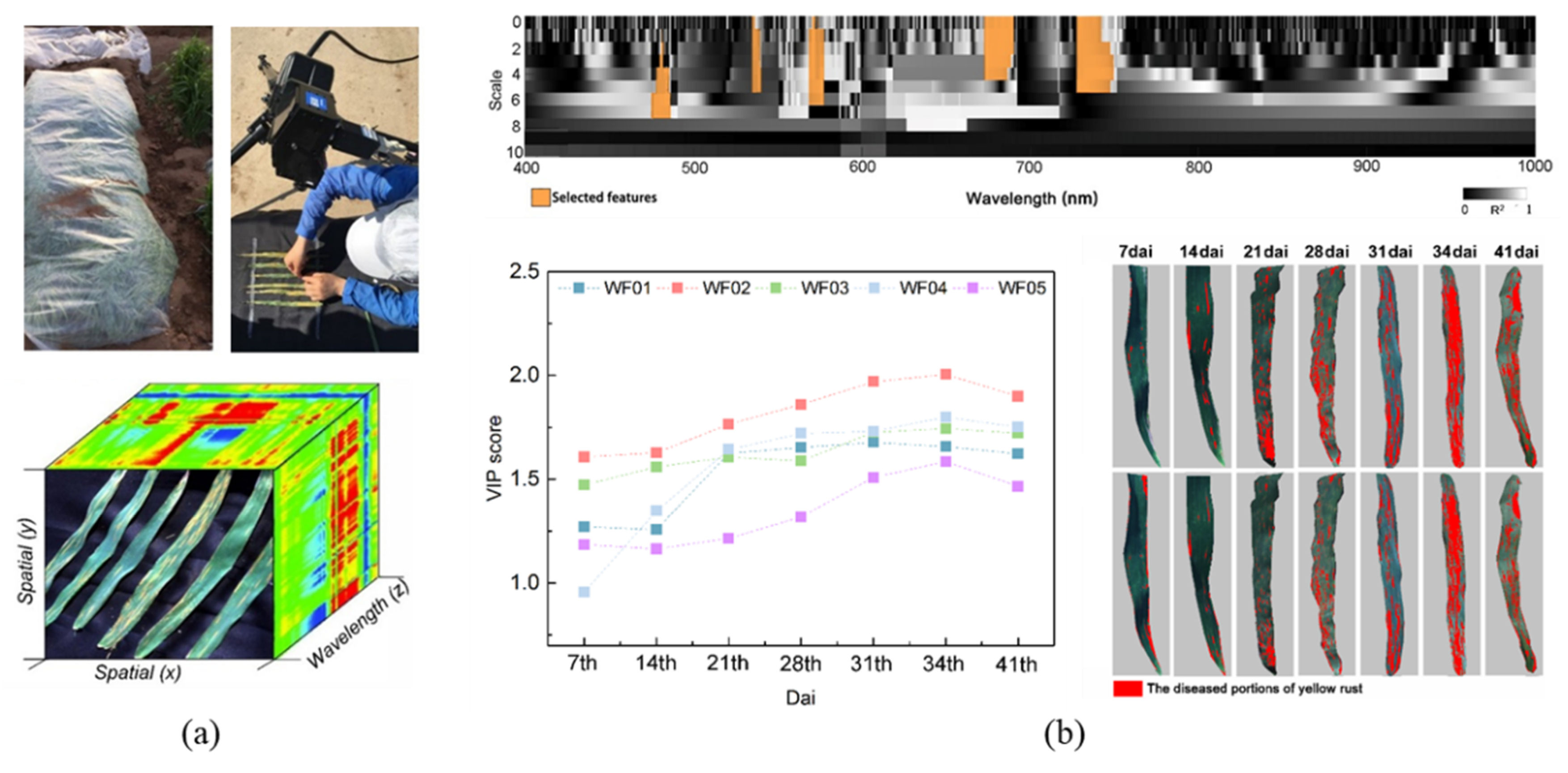
At the leaf scale, a series of in situ observations were conducted at the Scientific Research and Experimental Station of Chinese Academy of Agricultural Science (39°30′40” N, 116°36′20” E) in Langfang, Hebei province, China. The images with spectral information of wheat leaves (Figure 4a) were obtained by using a visible and near-infrared (VNIR) hyperspectral imager (Headwall VNIR imagining sensor, Headwall Photonics, Inc., Bolton, MA, USA). The wavelet features that have significant correlation with the severity of wheat yellow rust were extracted, and two monitoring models utilizing linear discriminant analysis (WRSF-LDA) and support vector machine (WRSF-SVM), respectively, were developed using the wavelet features as input (Figure 4b).
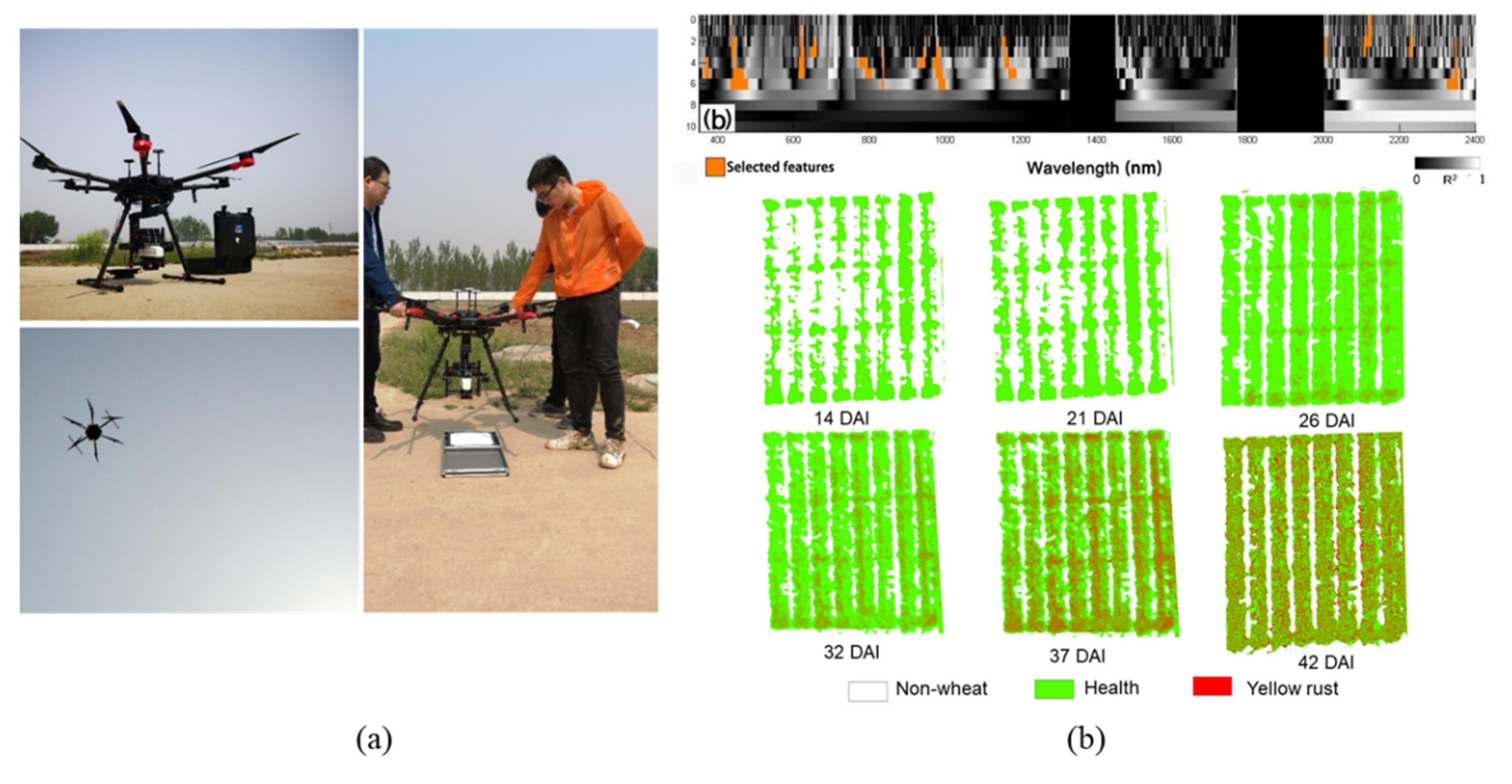
At the canopy scale, the field experiment was designed to acquire hyperspectral UAV images in the development of yellow rust. The experiment was also conducted at the Scientific Research and Experimental Station of Chinese Academy of Agricultural Science. The UAV used in the experiment was an M600 Pro aircraft of Daijang Innovations (DJI), and a Cubert S185 FireflEYE SE hyperspectral imaging camera was used (Figure 5a). Based on UAV hyperspectral images and field survey data, wavelet features and vegetation indices which were sensitive to yellow rust were extracted (Figure 5b). A kernel principal component analysis-based support vector machine model (KPCA-SVM) was proposed to monitor yellow rust by using the above features and indices. This model used kernel function to transform the original nonlinear feature space into a linearly separable space, and then find the occurrence area of wheat yellow rust.
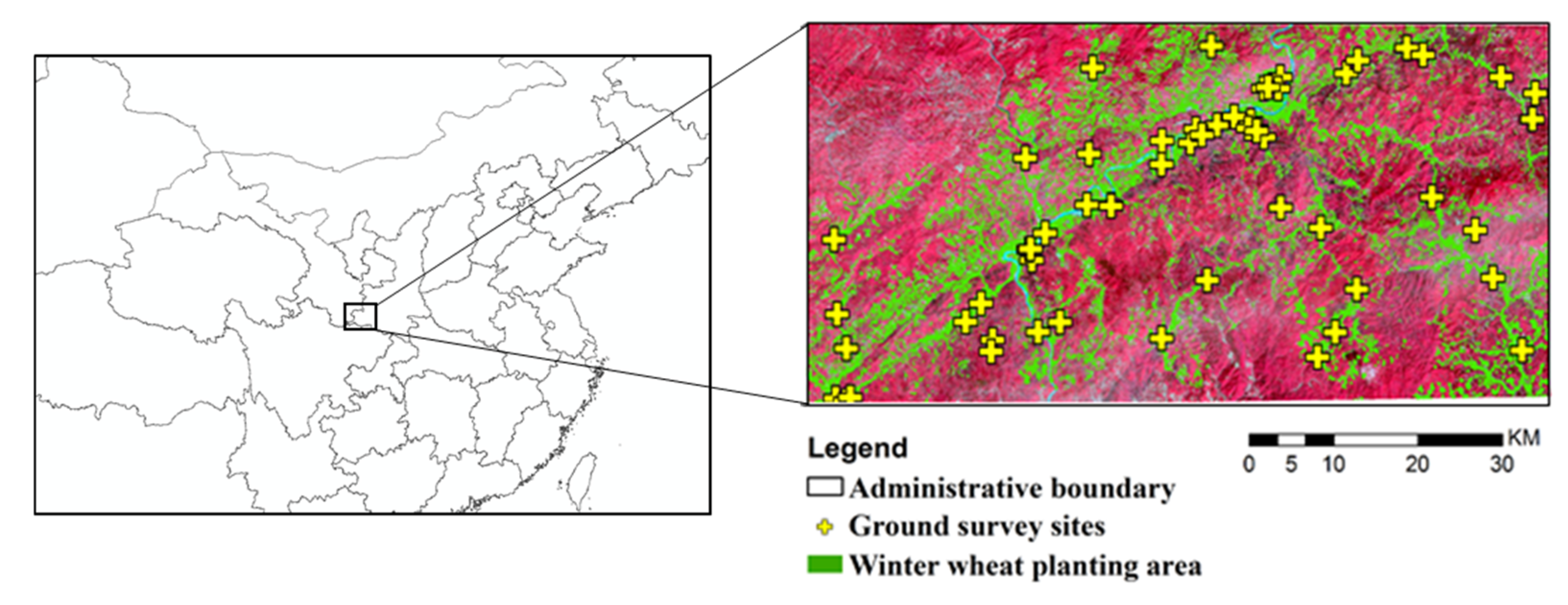
At the regional scale, satellite image data, meteorological data and field survey data were integrated to analyze the relationship between wheat yellow rust and the environment or the host, and then to develop a model for wheat yellow rust monitoring. For this study a satellite-ground synchronous field experiment was carried out in Ningqiang, Shaanxi province, China (Figure 6). The LAI and leaf chlorophyll content (LCC) of wheat infected by wheat yellow rust were measured using a LAI-2200 (Li-Cor Biosciences Inc., Lincoln, NE, USA) and a Dualex (FORCE-A, Inc., Orsay, France). The severity of wheat yellow rust of field samples was calculated based on the rules for monitoring and forecasting wheat yellow rust suggested by the National Plant Protection Department of China (Chinese Standard: GBT 15795-2011). Based on the experimental data and Sentinel-2 images acquired at the same time with the experiment, a wheat yellow rust monitoring model using fast Fourier transform technology was proposed. This model achieved accurate monitoring of wheat yellow rust through expressing the relationship between LAI and LCC and the severity of yellow rust.

3. Results

3.1. Coupling EO Data with Crop Models for Yield Prediction

The activity aims to test the performances of the EO data assimilation into biophysical crop models to improve durum wheat predictions.
The growing season of 2017–2018 in Maccarese (Italy) was used for calibration, obtaining a range of parameter values that represent a more realistic range for subsequent simulations. The following year (2018–2019) was used to test the efficiency of data assimilation on several wheat fields. EO imagery collected during the durum wheat growing season was aggregated by field, preprocessed, and used for data assimilation. For each field, the fitted LAI was assimilated into SAFY using EnKF, and a “standard” simulation without LAI assimilation (open loop) was also run (Figure 7). In addition to visual comparison of LAI trends, performance metrics were also calculated on yield (Table 2). LAI curves show a clear distinction between standard and EnKF simulations. The standard simulations of the five fields with wheat emerging in the first half of December (Figure 7a–e) generated almost identical LAI curves and, in turn, similar yield predictions. Indeed, initial conditions and meteorological forcing during the growing season were common to all the fields, and soil water limits were similar due to the homogeneity and low resolution of the ESDAC-JRC soil maps with respect to the farm dimensions. This resulted in similar simulations when EnKF was not used (open loop). In the other two fields (Figure 7f,g), durum wheat was sown and harvested earlier, and this was reflected by the LAI development. In all the cases, however, the EnKF procedure simulated LAI following almost exactly the curves fitted on Sentinel-2 data. This permitted adjusting the simulation trajectory daily, obtaining not only a better representation of LAI, but also a more realistic quantification of in-season biomass and yield growth. In fact, the validation on yield at the field level showed a three-fold improvement in yield estimations when EnKF was used, with respect to the standard simulation (Table 2).
The improvement in the simulation performances with data assimilation is testified by the lower discrepancies between predicted yield and yield measured by the combine harvester (lower RMSE, RRMSE and MAE). The data assimilation results are comparable to those of [13] for common wheat at the field scale in China. The authors obtained, over three years of experiments, an average RMSE of 1.1 t·ha−1. Their RRMSE (18%) was lower than in our case, however, probably due to a narrower range of the observed yield, approximately from 3 to 8 t·ha−1. In our case, durum wheat yield ranged from about 1 t·ha−1 to more than 8 t·ha−1.
The yield of the two fields with a shorter growing cycle (Figure 7f,g) was overestimated, probably due to the rather poor yield (1.1 and 1.4 t·ha−1), which is more difficult to simulate for a relatively simple model such as SAFY due to the involvement of various sources of stress (Figure 8). Crop models in general, including SAFY, are reported to perform poorly when yield is greatly limited by severe stress [48]. Lower yields can result from limitations that are rarely simulated by this kind of dynamic crop model, such as weeds, pests and diseases [49,50]. In another field the model showed poor performance despite the assimilation, simulating 2.7 t·ha−1 of grain yield with respect to the 5.7 t·ha−1 measured at harvest (Figure 7). The field was the largest, and showed a slow and uneven wheat growth that may not have been adequately caught with the use of a single LAI curve for the entire field.

3.2. Crop Diseases Results

3.2.1. Orchards Diseases Mapping

Having in mind the objective of assessing the possibility of monitoring the spread of diseases, Psa in this case, in permanent crops such as kiwi trees, by using EO satellite images, we focused on the analysis of RapidEye images to validate the results presented in [17]. In that work, multiple vegetation indices were generated and a binomial logistic regression was used to relate these vegetation indices to the presence of Psa. Psa data used in [17] were provided with some uncertainty about the actual infection date. In the present study, the data were reclassified, and the analysis was confined to KBIs (Kiwi Blocks identified by KVH) with either an ‘early’ (infected) or ‘control’ (non-infected) response. Taylor et al. [45] identified potential relationships between Psa infection and canopy vigour retrieved by remotely sensed imagery. However, they recognized that there were limitations in their study, particularly about the resolution at which the infection data was collected (orchard level rather than maturity level).
Initially, the study was carried out using RapidEye images, and an approach similar (in terms of VIs and NN) to the one used to study the New Zealand’s regions was adopted. Subsequently, we further investigated Sentinel-2 and PRISMA imagery by applying the above mentioned Vis.
Concerning the analysis carried out on the regions of New Zealand based on the RapidEye imagery of 2010 and 2012, the confusion matrix (Table 3) obtained by applying the NN shows an acceptable percentage of good classifications (AO higher than 69%).
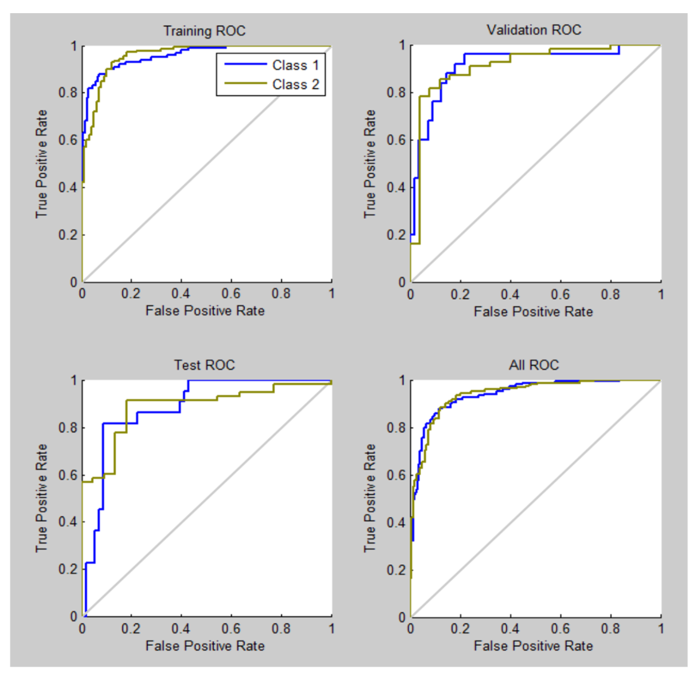
A way to measure how well the NN fits data is the receiver operating characteristic (ROC) plot. Figure 9 shows the relationship of false positive and true positive rates as the thresholding of outputs is varied from 0 to 1. The ROC curve shows the true positive rate versus false positive rate (equivalently, sensitivity versus 1–specificity) for different thresholds of the classifier output.
The results obtained from the second analysis, which included the same list of VIs applied previously, now extracted from Sentinel-2 images (Table 4), were obtained considering the health status of the orchards published by the biosecurity organization KVH in 2019. These results showed an improvement in the performance, highlighting the potential use of Sentinel-2 datasets for the detection of Psa outbreaks.
The datasets ingested into the NN included the statistics for each VI (as Maximum, Minimum, Mean and Standard deviation), for each block (or maturity area). After the addition of 250 blocks from Takaka region to the previously digitized 400 blocks from the Te Puke area, the classification performance improved, increasing the accuracy up to 95%.
The study on the New Zealand sites also included PRISMA hyperspectral imagery, which allowed adding a new set of VIs. The analysis was carried out on archived images of the areas that in 2019 were clearly identified as infected (Te Puke) and non-infected (South Island). A similar analysis, ongoing, aims at including a new set of PRISMA images, collected monthly, to assess the possibility for identifying the potential outbreaks at different phenological stages in the Agro Pontino region in Central Italy.
To improve the performance of the NN, a new set of VIs based on hyperspectral imagery was added. The NN was designed with similar characteristics to the previous analysis (20 hidden layers, 60% training, 20% validation, and 20% testing). In this case, the performance of the classifier was significantly improved, reaching values greater than 95% (Table 5 and Table 6).
The same NN, trained using the data on New-Zealand, was saved and applied to the area devoted to the cultivation of kiwi located in the Lazio Region of Italy, where the presence of this pest was already detected.
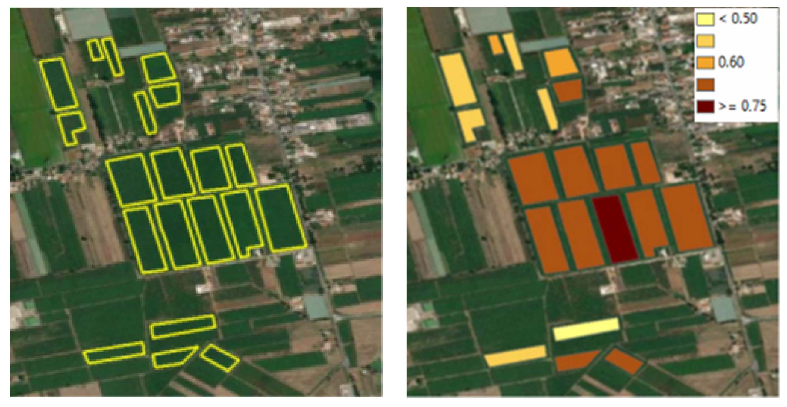
The NN was then fed with VIs extracted using the Rapideye images of the Agro Pontino. It can be noticed that certain blocks (or maturity areas) show similar responses and were classified under different levels of probability of infection (Figure 10).
Nevertheless, it is important to underline that the NN was trained considering only the presence of Psa (Pseudomonas syringae pv. Actinidiae) epidemics which have caused major economic losses to kiwifruit industry since 2007–2008, while, more recently, the Halyomorpha halys, also known as the brown marmorated stink bug, has seriously compromised fruit quality and marketable yields [46]).
For the test cases located in Italy, it could not be concluded that Psa was present in the fields, for which no ground data were available, but orchards showed a similar behavior to the fields of other regions which were identified as infected by Psa. Therefore, in the Agro Pontino case study, further field campaigns have to be carried out for validation purpose. This would help to improve the robustness of the current NN.
Despite the promising results as shown in Table 7, the performance of the NN for this case study could also be related to different phenology states of the orchards. Thus, a new analysis with new image acquisitions was programmed for the incoming seasons to validate and confirm these results.
It can be concluded that the methodology described above can be applied for the monitoring of kiwifruit anomalies, considering the availability of satellite images with the required spectral, radiometric and spatial resolution. However, the results cannot be directly applied to any kind of orchard, as further detailed in the Discussion section.
Concerning the use of hyperspectral images, it needs to be noted that, for performing this test, the images were collected in dates different from those of the RapidEye and Sentinel-2 images and, also, with a smaller number of fields, due to the limited time span of the archived PRISMA images, and the limited coverage of the areas of interest. Therefore, with the limitation recalled above, the result, not obvious because satellite images of different spatial resolution (in the range of 5 m to 30 m) and number of spectral channels were used, is that, in this case, in the range of spatial resolution from 5 m to 30 m, higher spectral information provides better results.

3.2.2. Wheat Yellow Rust Mapping

A primary aim of the research, taking wheat yellow rust as an example, was to use remote sensing technology to achieve accurate monitoring of crop diseases at different scales, thus providing a reference for the application of remote sensing technology in crop disease monitoring and forecasting. We have analyzed the pathogenesis and epidemiological process of wheat yellow rust and have developed a feature extraction method that is consistent with the pathological characteristics and epidemiological mechanism of this disease. Starting from the characteristics of the impact of wheat yellow rust on the physiological and biochemical indicators of wheat, parameters such as vegetation index and wavelet features were extracted, and the data characteristics at different scales were considered to construct monitoring models applicable to different scales.
At the leaf scale, a monitoring model based on wavelet features extracted from non-imaging hyperspectral data was developed. It was found that the wavelet features with strong correlation with disease severity were mainly distributed in the 480 nm–750 nm range. When the proportion of yellow rust spores in the leaf was small (4% to 19%), the average monitoring accuracy of the model was 70.1%. With the increase of yellow rust infestation time and area of yellow rust spores in the leaf, the spectrum of the leaf changed significantly, therefore providing more valuable information for disease monitoring and rapidly improving the monitoring accuracy of the model. The average monitoring accuracy of model was 86.3% when the proportion of yellow rust spore in the leaf was more than 40%. Table 8 shows the change in the average monitoring accuracy of the model after yellow rust infestation.
At the canopy scale, wavelet features and vegetation indices with high correlations with disease severity were extracted using UAV hyperspectral images, and then applied to construct the disease monitoring model. The results of the analysis showed that the monitoring accuracy of the applied model tended to increase, and then decrease, as the development of yellow rust progressed. The monitoring accuracy (Table 9) ranged from 88.7% to 99.2% for healthy samples and 84.2% to 100% for diseased samples. The highest monitoring accuracy of the model was achieved for 31 days after the infection, with 99.2% and 100% of identification accuracy for healthy and diseased samples, respectively. The results of this study showed that accurate monitoring of wheat yellow rust at the canopy scale can be achieved using UAV hyperspectral imagery.
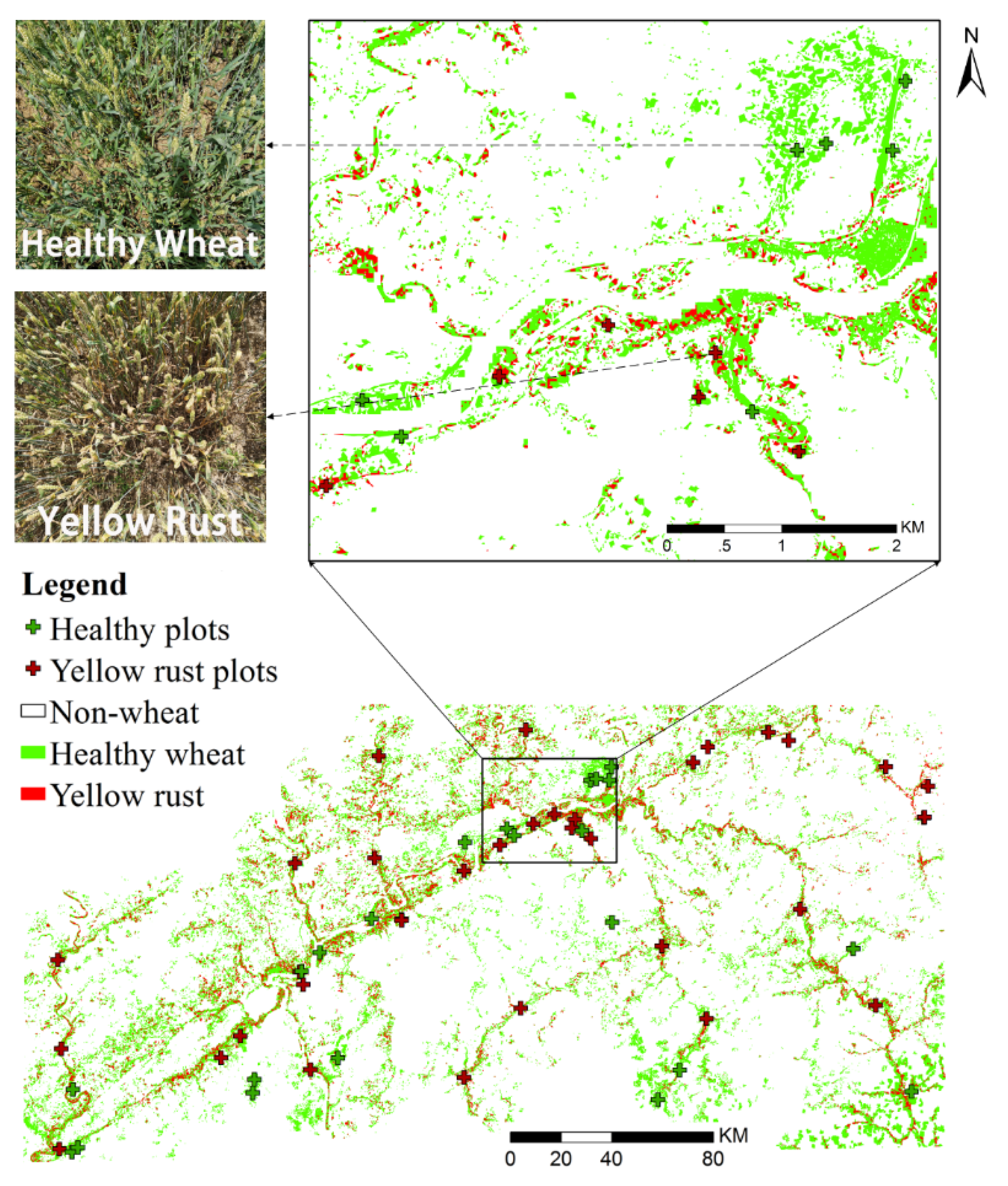
At the regional scale, spectral indices sensitive to LAI and LCC were constructed based on disease-sensitive spectral bands at the leaf and canopy scale, and then the yellow rust monitoring model KPCA-SVM was developed. The monitoring results are shown in Figure 11. The model monitoring results were generally consistent with our field survey. Wheat yellow rust mainly occurred around the Jialing River in Ningqiang county, an area that provides ideal environmental conditions for the infection and development of yellow rust. Table 10 gives the confusion matrix and kappa value corresponding to the monitoring results. It can be found that the overall accuracy of the monitoring model is 84.4% and the kappa coefficient is 0.742, thus achieving accurate monitoring of yellow rust.
These results suggest that remote sensing monitoring of wheat yellow rust at leaf, canopy and regional scales is feasible. When developing the monitoring model, information on the spatial and temporal variation of spectral features is the basis for small-scale disease monitoring. As the monitoring scale rises, crop growth and environmental information needs to be added into the spectral feature set to achieve more accurate disease monitoring. The results show that there is consistency in the sensitive spectral bands of diseases at the leaf scale and canopy scale, and the regional scale disease monitoring model developed based on the sensitive spectral bands also achieved accurate monitoring. The disease monitoring methods and results presented in this section can provide a reference for subsequent research of remote sensing monitoring of crop pests and diseases.

4. Discussion

Joining EO data and crop models through data assimilation proved to be an efficient approach to predict durum wheat yield. The results obtained at the Maccarese site provided three take home messages that are worth mentioning, considering the state of the art of EO studies and of previous works on similar topics. Firstly, yield was predicted by exploiting both EO data and crop models. Both methods have strength and weaknesses, but data assimilation is an efficient tool to get the best of both worlds [10]. Using optical EO data only has a limited applicability for the prediction of crop yield, since yield is an indirect property that, contrarily to canopy properties such as LAI, cannot usually be estimated solely by EO retrieval [10]. Conversely, process-based crop models can simulate complex processes of plant growth and development (and yield formation) by using well-established scientific concepts in the form of mathematical equations, but require some adjustment to real field measurements to obtain reliable results. A process-based approach of dynamic crop models can integrate the EO data with functions for the estimation of crop growth and yield that have general validity [50,51]. Secondly, the combination of models and EO-retrieved LAI permitted the prediction of yield without requiring field work. The only information collected in the field was durum wheat yield, measured by the combine harvester. Extensive field data would have been required for calibration either with empirical methods based on regression to directly estimate yield from EO data [10], or with a crop model (such as SAFY) used without data assimilation [38]. Data assimilation permitted avoiding field work and at the same time reduced uncertainties in the simulations. Thirdly, so far SAFY has been used with data assimilation mostly for regional scale yield estimations [11,15], but the experiment at Maccarese allowed for testing the performances of this method at the field scale. This highlighted that yield can be satisfactorily predicted at the field level, especially in an agricultural context such as the Italian one, where field dimensions are often of few hectares and simulations can be carried out at the field level. This first step in this direction opens the door for potential applications of the EO–model combination to plan crop management at the field or within-field scale and adjust it with in-season information. Several approaches can be used to exploit EO data to identify homogeneous management zones in crop fields [52], and crop models can be applied to these zones to plan agronomic management practices and adjust them during the season when new information is available, for example by applying variable rates of N based on the productive potential of each zone [53]. Coupling EO data with modeling approaches can also be used for in-season adjustments of irrigation plans of variable rate irrigation management zones [54]. All these applications primarily require accurate crop growth and development estimates that need little or no field work and that can be adjusted during the season when new EO data become available [55].
The mapping of potential anomalies on agricultural crops (i.e., winter wheat and maize), orchards and particular trees from a worldwide perspective is technically feasible thanks to the present generation and availability of EO based products that can systematically cover large areas of interest. Remote sensing images are widely used to study vegetation status, and can be a real aid in monitoring activities, especially to support localized field surveys. Non-invasive methods carried out with the assistance of remote sensing technologies can be fully exploited to assess the current situation of entire regions of interest, evidencing areas under potential risks, and also under different climate change contexts. The mapping of diseased crops based on automatic analysis of remote sensing data could be a valuable support for in situ investigation planning. In fact, the model shown in Section 2.2.2 achieved accurate monitoring of wheat yellow rust, by exploiting the relationship between LAI and LCC and the severity of yellow rust. Such a model, based on proximal sensing hyperspectral data, aims at defining a possible procedure for detecting crop pests and diseases to be applied to hyperspectral satellite images, for which atmospheric and spatial resolution effects should be considered. Satellite imagery allows covering a large area of interest at an affordable cost.
The example for the application of remotely sensed images, at different spatial and spectral resolution, for detecting the presence of the Psa disease in kiwifruit trees shows that the accuracy of the classification is mainly depending on the spectral channels rather than on the spatial resolution. In fact, the best results, shown in Table 7, are obtained by using PRISMA hyperspectral images which have 30 m spatial resolution. Of course, the spatial resolution should be compatible with the size of the orchards’ field, that is, the spatial resolution of the satellite images exploited here spans from 5 m to 30 m. Further, it should be underlined that the good results obtained by applying a NN based on statistical parameters extracted by vegetation indices could be due to the distribution of kiwi trees. In fact, kiwifruit vines are organized to form a pergola that provides a single plane canopy; therefore, the monitoring is only minimally affected by the characteristics of soil or the presence of grass on the surface around the trees. As matter of the fact, an approach based on NDVI was applied to detect the presence of olive groves affected by Kf [21]. In that case, the selection of the images for carrying out the analysis would have considered the background grass phenology because, in that case, trees are distributed roughly 6 m apart, so that surface cover is visible and can affect the NDVI estimate. This research topic is currently actively growing, achieving new and promising results, in line with climate change scenarios which predict a higher incidence of plant pathogens. In this continuous changing context, further developments should be considered to act timely and prevent the spread of emerging pests. Plant diseases’ epidemiology is affected by three factors (the disease triangle): the host plant, the pathogen and the vector, all influenced by environmental conditions. Therefore, further studies are focusing on the vectors and their dynamics, the environmental conditions for their growth and on the detection of the weather patterns that could leverage the development and diffusion of pest outbreaks.
Crop disease monitoring from Earth Observation is an important topic in the development of precision agriculture. This paper presents remote sensing monitoring methods and results for wheat yellow rust at multiple scales. Monitoring accuracy appeared first to increase, and then to decrease, with the progression and spread of the disease. The improvement of monitoring accuracy was mainly due to the increase in the proportion of yellow rust spores in the leaf, which provide more spectral change information and can enhance the model’s ability to identify the disease. The subsequent decrease in monitoring accuracy may be due to the natural wilting process of leaves brings noise to the spectral features of the disease, and thus reduces the ability of the model to identify yellow rust. This phenomenon indicates that there is an optimal time for disease monitoring. In a disease control process, the appropriate time should be selected for disease monitoring based on the physiological characteristics of the disease. In terms of the sensitive bands of the disease, there is consistency at the leaf scale and canopy scale, and the disease monitoring model developed based on the sensitive bands has good performance in the monitoring of yellow rust when using Sentinel-2 images. These results indicate that the bands more sensitive to the disease, identified at the leaf scale on the ground, can be transferred to large scale disease monitoring. However, since the pixels of satellite images contain complex information, regional-scale disease monitoring should combine spectral information with meteorological and environmental information to develop a more comprehensive monitoring model.

5. Conclusions

Agriculture is one of the major domains in which EO data can be successfully applied in a diversity of agronomical applications, e.g., to optimize the use of chemicals and fertilizer, to foster optimal agronomical practices, and to increase yield and quality production. This domain is a common research issue for both EU and Chinese researchers, since it is formed by an ensemble of operational needs connected to food security and also related to production, prediction and crop diseases, which can affect worldwide food availability. The methodologies, resources and tools applied in the current study, moreover, aim at answering to some of the requirements declared by the European Food Safety Authority [56] concerning the identification of areas of high disease risk where to target the surveys, and the development of detection methodologies and reporting procedures to derive the potential for early detection and monitoring of new outbreaks.
This manuscript aims to summarize the effort performed by the SINO-EU research Team, in the framework of the ESA Dragon4 initiative successfully concluded in 2020, for a full exploitation of the Chinese-European EO resources in relation to agricultural applications suitable for both local and regional scales. Most of our effort was addressed to the analysis of the EO data to retrieve, with a suitable accuracy, biophysical and biochemical variables related to crop functioning and photosynthesis.
Results show that wheat yield was predicted with a lower RMSE with respect to the standard simulation (e.g., 1.42 t·ha−1 instead of 4.42 t·ha−1) by applying the EnkF assimilation procedure into the SAFY crop model to assimilate LAI values. Regarding the detection of orchards’ pathogens, an overall accuracy higher than 95% was achieved by training a NN algorithm. Concerning wheat yellow rust detection, an overall classification accuracy of 89.3% was obtained when applying a WRSF-SVM classification procedure.
The research studies performed by the SINO-EU teams still require further steps to minimize the discrepancies between models and data sources when applied at different scales, having also in mind the specificity of the different environments pertaining to EU and China. These studies will constitute a heritage to the ongoing activities in the Dragon-5 program initiative. In this framework, further studies will be addressed to:
(a)
Expand the estimation of new variables, by exploring the RTM code PROSPECT-PRO (e.g., for proteins and nitrogen);
(b)
Exploit the newly operative hyperspectral missions for their application on a regional base to detect pathogens;
(c)
The implementation of machine/deep learning techniques for the generalization of the pre-operative chains applicable to the local scale for agricultural applications.
Further studies will be devoted to exploiting the newly available high spectral resolution satellite data, such as those coming from GF5, PRISMA, EnMAP and, in the future, from SBG and CHIME hyperspectral missions.

Author Contributions

S.P. (Stefano Pignatti), R.C., G.L. and W.H. designed the conceptual framework of this research; Z.L. analyzed the data regarding the grain quality; P.M. performed the data analysis for the permanent crops’ diseases, L.L. contributed to the identification of pathogens on cereal; N.M. RTM retrieval and data analysis; S.P. (Simone Pascucci) acquired and analyzed the field data, contributed to the revision process of the results obtained and reviewed the manuscript. P.C.S. contributed to the data assimilation software and data analysis; M.T. was in charge to the SAFY assimilation experiment; D.U. RTM retrieval with hybrid approaches; H.Y. data analysis; G.Y. designed the conceptual framework of this research. All authors have read and agreed to the published version of the manuscript.

Funding

This research was partially funded byDragon4, ESA contract No. 4000121195/17/I-NB.

Institutional Review Board Statement

Not applicable.

Informed Consent Statement

Informed consent was obtained from all subjects involved in the study.

Data Availability Statement

Not applicable.

Acknowledgments

This research was also supported by ASI with project PRISCAV, and ESA project Hyperspectral Imaging Mission Concept.

Conflicts of Interest

The authors declare no conflict of interest.

Appendix A. Simple Algorithm for Yield Estimates (SAFY)

In SAFYsw, biomass accumulation depends on the amount of Photosynthetically Active Radiation (PAR) that is absorbed by the canopy, following Equation (A1):
∆DAM = Rg∙εC∙εl∙ELUE∙FT(Ta)∙Ks,
where Rg is the solar radiation, εC is the climatic efficiency, εl is the light efficiency, ELUE the effective light use efficiency, which also accounts for stresses not considered in the other crop modules, and FT is the temperature stress. Ks is the water stress coefficient (an addition of the SAFYsw version of the model), which acts as a modifier of the biomass accumulation. Ks is derived from the actual transpiration to potential transpiration ratio, which are calculated in the water balance module, as specified below. Daily LAI expansion is calculated from the daily accumulated biomass until senescence as in Equation (A2):
∆GLAI+ = ∆DAM∙PL(∑Ta)∙SLA,
where ∆GLAI+ is the LAI expansion, PL(∑Ta) is a partition-to-leaf function calculated from the thermal sum and two partition parameters (PLa and PLb), and SLA is the specific leaf area. After reaching a thermal sum threshold defined by the senescence parameter STT, the LAI starts decreasing following Equation (A3):
∆GLAI- = GLAI∙(∑Ta-STT)/Rs,
where Rs is the canopy senescence rate. When canopy expansion ends, grain starts accumulating depending on the Py parameter of partition to grain and on the total biomass so far accumulated, as in Equation (A4):
∆GY = DAM∙Py.
The SAFYsw version also adds a water balance based on the tipping bucket approach by [38], where an upward flux (evapotranspiration-driven) and a drainage downward flux (gravity-driven) are calculated. An equilibrium evaporation rate (EET) is calculated through the Priestley-Taylor equilibrium equation, using albedo (α), solar radiation and daytime temperature (T), as in Equation (A5):
EET = Rg∙(0.0045 − 0.00437∙α)∙(T + 29).
Following [38], potential evapotranspiration (ETp) is 1.1 times EET, and potential soil evaporation (Ep, Equations (A6) and (A7) and potential plant transpiration (Tp, Equations (A8) and (A9) are then calculated considering specific LAI thresholds:
Ep = ETp∙(1 − 0.43∙LAI); with LAI < 1,
Ep = ETp∙exp(−0.4∙LAI); with LAI ≥ 1,
Tp = ETp∙(LAI/3); with LAI < 3,
Tp = ETp; with LAI ≥ 3.
Potential root water uptake (RWU) is dependent on water available in each layer above the lower limit of plant water availability (LL, i.e., the wilting point), and is calculated as in Equation (A10):
RWU(l) = 0.00267∙exp(62∙(SW(l) − LL(l)))/(6.68 − ln(RLV(l)))
where l indicates the layer, SW(l) is the soil water content and RLV(l) is the root length density. With a total RWU ≥ of Tp, the actual water uptake is considered equal to potential transpiration (no water stress, actual transpiration equals potential transpiration, Ta = Tp). Otherwise, the transpiration demand is not satisfied and Ta is set equal to the actual uptake (limited by soil water availability), and a water stress coefficient (Ks) is calculated as the ratio Ta/Tp. Ks is used as a linear modifier of biomass accumulation in Equation (A1).
The downward flux occurs from a soil layer when the soil water content is above the drained upper limit (DUL, i.e., field capacity). The excess water is transferred downward to the following layers according to a fraction of the difference between saturation (SAT) and DUL and to a drainage coefficient (SWCON) that accounts for the infiltrability simplified in Equation (A11):
Drain(l) = SWCON∙(SW(l) − DUL(l))∙Depth(l)
Soil water content is calculated daily for each layer from the balance of the upward and downward fluxes.

Appendix B. The Ensemble Kalman Filter (EnKF) Assimilation Procedure

The EnKF steps used in the data assimilation of the Maccarese study can be summarized as follows:
  • Initialization of the model ensemble: an ensemble of N model simulations (N = 100 in our case) was generated. Each element of the ensemble was obtained by creating a different set of model parameters. Some parameters were considered fixed (Table 1), while for the calibrated parameters a value was randomly sampled from a truncated gaussian distribution with fixed average and lower and upper limits corresponding to the range obtained during the calibration (Table 1). This perturbation allows for the simulation of the error covariance.
  • Forecast step: a simulation was run with a daily timestep separately for each element of the model ensemble, till the day of observation, to obtain an ensemble of simulated LAI values. The error covariance of the forecast can be calculated from the ensemble as in Equation (A12):
    (PE)tf = (Xt − E|Xt|)∙(Xt − E|Xt|)T/(N − 1),
    where (PE)tf is the error covariance of the ensemble of forecasts at time t, E|Xt| the ensemble of model state variables (LAI in this case) at time t, and Xt is the simulated LAI mean value.
  • Observation error propagation: an ensemble of N LAI observations was generated for each day with a LAI observation (in our case, each day of the growth cycle, due to the LAI fitting procedure). The ensemble was obtained by randomly sampling from a gaussian distribution with an average equal to the EO-derived LAI value and a standard deviation of 10%. Similarly, to the simulated values, the error covariance of the observation can be calculated from the ensemble as in Equation (A13):
    (RE)tf = (Yt − E|Yt|)∙(Yt − E|Yt|)T/(N − 1),
    where (RE)tf is the error covariance of the ensemble of observations at time t, E|Yt| the ensemble of observations and Yt the original mean value.
  • Update step: the mean state and the model state covariances are updated using the Kalman gain (for each ensemble element) following Equation (A14):
    Kt = Ptf∙HT∙(H∙Ptf∙HT + Rt)−1,
    where Kt is the Kalman gain at time t, Ptf is the model state forecast at time t, H is the observation operator, assumed constant over time, Rt is the measurement error at time t.
    The mean state was (Equation (A15)):
    xta = xtf + Kt∙(yt − Hxtf),
    where xta is the updated mean state, obtained from the combination of the model forecast mean state xtf, the observation mean xtf, and the Kalman gain.
    The model state covariance at time t (Pta) is expressed by Equation (A16):
    Pta = (I − Kt∙H)∙Ptf,
    where I is the identity matrix.
  • The forecast, observation error propagation and update steps were repeated recursively till the end of the simulation, assimilating each new observation.

References

  1. Jia, K.; Wu, B.; Li, Q. Crop classification using HJ satellite multispectral data in the North China Plain. J. Appl. Remote Sens. 2013, 7, 073576. [Google Scholar] [CrossRef]
  2. Whitcraft, A.K.; Becker-Reshef, I.; Killough, B.D.; Justice, C.O. Meeting earth observation requirements for global agricultural monitoring: An evaluation of the revisit capabilities of current and planned moderate resolution optical earth observing missions. Remote Sens. 2015, 7, 1482–1503. [Google Scholar] [CrossRef] [Green Version]
  3. Ozdarici-Ok, A.; Ok, A.O.; Schindler, K. Mapping of agricultural crops from single high-resolution multispectral images—Data-driven smoothing vs. parcel-based smoothing. Remote Sens. 2015, 7, 5611–5638. [Google Scholar] [CrossRef] [Green Version]
  4. Zhou, T.; Pan, J.; Zhang, P.; Wei, S.; Han, T. Mapping Winter Wheat with Multi-Temporal SAR and Optical Images in an Urban Agricultural Region. Sensors 2017, 17, 1210. [Google Scholar] [CrossRef] [PubMed]
  5. Veloso, A.; Mermoz, S.; Bouvet, A.; Le Toan, T.; Planells, M.; Dejoux, J.F.; Ceschia, E. Understanding the temporal behavior of crops using Sentinel-1 and Sentinel-2-like data for agricultural applications. Remote Sens. Environ. 2017, 199, 415–426. [Google Scholar] [CrossRef]
  6. Brook, A.; De Micco, V.; Battipaglia, G.; Erbaggio, A.; Ludeno, G.; Catapano, I.; Bonfante, A. A smart multiple spatial and temporal resolution system to support precision agriculture from satellite images: Proof of concept on Aglianico vineyard. Remote Sens. Environ. 2020, 240, 111679. [Google Scholar] [CrossRef]
  7. Zhang, L.; Zhang, Z.; Luo, Y.; Cao, J.; Tao, F. Combining Optical, Fluorescence, Thermal Satellite, and Environmental Data to Predict County-Level Maize Yield in China Using Machine Learning Approaches. Remote Sens. 2019, 12, 21. [Google Scholar] [CrossRef] [Green Version]
  8. Zhao, L.; Huang, W.; Chen, J.; Dong, Y.; Ren, B.; Geng, Y. Land use/cover changes in the Oriental migratory locust area of China: Implications for ecological control and monitoring of locust area. Agric. Ecosyst. Environ. 2020, 303, 107110. [Google Scholar] [CrossRef]
  9. Zhou, X.; Zhang, J.; Chen, D.; Huang, Y.; Kong, W.; Yuan, L.; Ye, H.; Huang, W. Assessment of Leaf Chlorophyll Content Models for Winter Wheat Using Landsat-8 Multispectral Remote Sensing Data. Remote Sens. 2020, 12, 2574. [Google Scholar] [CrossRef]
  10. Weiss, M.; Jacob, F.; Duveiller, G. Remote sensing for agricultural applications: A meta-review. Remote Sens. Environ. 2020, 236, 111402. [Google Scholar] [CrossRef]
  11. Silvestro, P.C.; Pignatti, S.; Pascucci, S.; Yang, H.; Li, Z.; Yang, G.; Huang, W.; Casa, R. Estimating Wheat Yield in China at the Field and District Scale from the Assimilation of Satellite Data into the Aquacrop and Simple Algorithm for Yield (SAFY) Models. Remote Sens. 2017, 9, 509. [Google Scholar] [CrossRef] [Green Version]
  12. Guo, C.; Tang, Y.; Lu, J.; Zhu, Y.; Cao, W.; Cheng, T.; Zhang, L.; Tian, Y. Predicting wheat productivity: Integrating time series of vegetation indices into crop modeling via sequential assimilation. Agric. For. Meteorol. 2019, 272, 69–80. [Google Scholar] [CrossRef]
  13. Duchemin, B.; Maisongrande, P.; Boulet, G.; Benhadj, I. A simple algorithm for yield estimates: Evaluation for semi-arid irrigated winter wheat monitored with green leaf area index. Environ. Model. Softw. 2008, 23, 876–892. [Google Scholar] [CrossRef] [Green Version]
  14. Upreti, D.; Pignatti, S.; Pascucci, S.; Tolomio, M.; Li, Z.; Huang, W.; Casa, R. A Comparison of Moment-Independent and Variance-Based Global Sensitivity Analysis Approaches for Wheat Yield Estimation with the Aquacrop-OS Model. Agronomy 2020, 10, 607. [Google Scholar] [CrossRef]
  15. Upreti, D.; Pignatti, S.; Pascucci, S.; Tolomio, M.; Huang, W.; Casa, R. Bayesian Calibration of the Aquacrop-OS Model for Durum Wheat by Assimilation of Canopy Cover Retrieved from VENµS Satellite Data. Remote Sens. 2020, 12, 2666. [Google Scholar] [CrossRef]
  16. Li, Z.; Taylor, J.; Yang, H.; Casa, R.; Jin, X.; Li, Z.; Song, X.; Yang, G. A hierarchical interannual wheat yield and grain protein prediction model using spectral vegetative indices and meteorological data. Field Crop. Res. 2020, 248, 107711. [Google Scholar] [CrossRef]
  17. Dong, Y.; Xu, F.; Liu, L.; Du, X.; Ren, B.; Guo, A.; Geng, Y.; Ruan, C.; Ye, H.; Huang, W.; et al. Automatic System for Crop Pest and Disease Dynamic Monitoring and Early Forecasting. IEEE J. Sel. Top. Appl. Earth Obs. Remote. Sens. 2020, 13, 4410–4418. [Google Scholar] [CrossRef]
  18. Guo, A.; Huang, W.; Ye, H.; Dong, Y.; Ma, H.; Ren, Y.; Ruan, C. Identification of Wheat Yellow Rust Using Spectral and Texture Features of Hyperspectral Images. Remote Sens. 2020, 12, 1419. [Google Scholar] [CrossRef]
  19. Ma, H.; Huang, W.; Jing, Y.; Pignatti, S.; Laneve, G.; Dong, Y.; Ye, H.; Liu, L.; Guo, A.; Jiang, J. Identification of Fusarium Head Blight in Winter Wheat Ears Using Continuous Wavelet Analysis. Sensors 2019, 20, 20. [Google Scholar] [CrossRef] [Green Version]
  20. Liu, L.; Dong, Y.; Huang, W.; Du, X.; Ma, H. Monitoring Wheat Fusarium Head Blight Using Unmanned Aerial Vehicle Hyperspectral Imagery. Remote Sens. 2020, 12, 3811. [Google Scholar] [CrossRef]
  21. Loizzo, R.; Guarini, R.; Longo, F.; Scopa, T.; Formaro, R.; Facchinetti, C.; Varacalli, G. Prisma: The Italian Hyperspectral Mission. In Proceedings of the IGARSS 2018-2018 IEEE International Geoscience and Remote Sensing Symposium, Valencia, Spain, 22–27 July 2018; pp. 175–178. [Google Scholar]
  22. Ren, K.; Sun, W.; Meng, X.; Yang, G.; Du, Q. Fusing China GF-5 Hyperspectral Data with GF-1, GF-2 and Sentinel-2A Multispectral Data: Which Methods Should Be Used? Remote Sens. 2020, 12, 882. [Google Scholar] [CrossRef] [Green Version]
  23. Matsunaga, T.; Iwasaki, A.; Tsuchida, S.; Iwao, K.; Tanii, J.; Kashimura, O.; Nakamura, R.; Yamamoto, H.; Kato, S.; Obata, K.; et al. Current status of Hyperspectral Imager Suite (HISUI) onboard International Space Station (ISS). In Proceedings of the 2017 IEEE International Geoscience and Remote Sensing Symposium (IGARSS), Fort Worth, TX, USA, 23–28 July 2017; pp. 443–446. [Google Scholar]
  24. Mahalingam, S.; Srinivas, P.; Devi, P.K.; Sita, D.; Das, S.K.; Leela, T.S.; Venkataraman, V.R. Reflectance based vicarious calibration of HySIS sensors and spectral stability study over pseudo-invariant sites. In Proceedings of the IEEE Recent Advances in Geoscience and Remote Sensing: Technologies, Standards and Applications (TENGARSS), Grand Hyatt Kochi Bolgatti, Kerala, India, 17–20 October 2019; pp. 132–136. [Google Scholar]
  25. Alonso, K.; Bachmann, M.; Burch, K.; Carmona, E.; Cerra, D.; Reyes, R.D.L.; Dietrich, D.; Heiden, U.; Hölderlin, A.; Ickes, J.; et al. Data Products, Quality and Validation of the DLR Earth Sensing Imaging Spectrometer (DESIS). Sensors 2019, 19, 4471. [Google Scholar] [CrossRef] [PubMed] [Green Version]
  26. Guanter, L.; Kaufmann, H.; Segl, K.; Foerster, S.; Rogass, C.; Chabrillat, S.; Hollstein, A.; Rossner, G.; Chlebek, C.; Sang, B.; et al. The EnMAP spaceborne imaging spectroscopy mission for earth observation. Remote Sens. 2015, 7, 8830–8857. [Google Scholar] [CrossRef] [Green Version]
  27. Boccia, V.; Adams, J.; Thome, K.J.; Turpie, K.R.; Kokaly, R.; Bouvet, M.; Green, R.O.; Rast, M. NASA-ESA Cooperation on the SBG and CHIME Hyperspectral Satellite Missions: A roadmap for the joint Working Group on Cal/Val activities (No. EGU21-15166). In EGU General Assembly Conference Abstracts; The European Geosciences Union: San Francisco, CA, USA, 2021. [Google Scholar]
  28. Zeng, L.; Wardlow, B.D.; Xiang, D.; Hu, S.; Li, D. A review of vegetation phenological metrics extraction using time-series, multispectral satellite data. Remote Sens. Environ. 2020, 237, 111511. [Google Scholar] [CrossRef]
  29. Beck, P.S.; Atzberger, C.; Høgda, K.A.; Johansen, B.; Skidmore, A.K. Improved monitoring of vegetation dynamics at very high latitudes: A new method using MODIS NDVI. Remote Sens. Environ. 2006, 100, 321–334. [Google Scholar] [CrossRef]
  30. Elmore, A.J.; Guinn, S.M.; Minsley, B.J.; Richardson, A.D. Landscape controls on the timing of spring, autumn, and growing season length in mid-Atlantic forests. Glob. Change Biol. 2012, 18, 656–674. [Google Scholar] [CrossRef] [Green Version]
  31. Gu, L.; Post, W.M.; Baldocchi, D.D.; Black, T.A.; Suyker, A.E.; Verma, S.B.; Vesala, T.; Wofsy, S.C. Characterizing the seasonal dynamics of plant community photosynthesis across a range of vegetation types. In Phenology of Ecosystem Processes; Noormets, A., Ed.; Springer: New York, NY, USA, 2009; pp. 35–58. [Google Scholar]
  32. Ballabio, C.; Panagos, P.; Monatanarella, L. Mapping topsoil physical properties at European scale using the LUCAS database. Geoderma 2016, 261, 110–123. [Google Scholar] [CrossRef]
  33. Ritchie, J.T.; Gerakis, A.; Suleiman, A. Simple model to estimate field-measured soil water limits. Trans. ASAE 1999, 42, 1609. [Google Scholar] [CrossRef]
  34. Jones, J.W.; Hoogenboom, G.; Porter, C.H.; Boote, K.J.; Batchelor, W.D.; Hunt, L.A.; Wilkens, P.A.; Singh, P.; Gijsman, A.J.; Ritchie, J.T. The DSSAT cropping system model. Eur. J. Agron. 2003, 18, 235–265. [Google Scholar] [CrossRef]
  35. Monteith, J.L. Solar radiation and productivity in tropical ecosystems. J. Appl. Ecol. 1972, 9, 747–766. [Google Scholar] [CrossRef] [Green Version]
  36. Monteith, J.L. Climate and the efficiency of crop production in Britain. Philos. Trans. R. Soc. Lond. B Biol. Sci. 1977, 281, 277–294. [Google Scholar]
  37. Trudgill, D.L.; Honek, A.; Li, D.; Van Straalen, N.M. Thermal time—Concepts and utility. Ann. Appl. Biol. 2005, 146, 1–14. [Google Scholar] [CrossRef]
  38. Wallach, D.; Makowski, D.; Jones, J.W.; Brun, F. Working with Dynamic Crop Models: Methods, Tools and Examples for Agriculture and Environment, 2nd ed.; Academic Press: London, UK, 2014; ISBN 978-0-12-397008-4. [Google Scholar]
  39. Kalman, R.E. A new approach to linear filtering and prediction problems. J. Basic Eng. 1960, 82, 35–45. [Google Scholar] [CrossRef] [Green Version]
  40. The MathWorks, Inc, MATLAB (Version R2019b, Academic Use). 2019. Available online: https://www.mathworks.com/ (accessed on 1 April 2021).
  41. Kang, Y.; Özdoğan, M. Field-level crop yield mapping with Landsat using a hierarchical data assimilation approach. Remote Sens. Environ. 2019, 228, 144–163. [Google Scholar] [CrossRef]
  42. Greer, G.; Saunders, C. The costs of Psa-V to the New Zealand Kiwifruit Industry and the Wider Community; Agribusiness and Economics Research Unit 62: Lincoln, New Zealand, 2012. [Google Scholar]
  43. Laneve, G.; Luciani, R.; Marzialetti, P.; Pignatti, S.; Huang, W.; Shi, Y.; Dong, Y.; Ye, H. Dragon 4—Satellite based analysis of diseases on permanent and row crops in Italy and China. J. Geod. Geoinf. Sci. 2020, 3, 107–118. [Google Scholar]
  44. Vanneste, J.L.; Giovanardi, D.; Yu, J.; Cornish, D.A.; Kay, C.; Spinelli, F.; Stefani, E. Detection of Pseudomonas syringae pv. actinidiae in kiwifruit pollen samples. N. Z. Plant Prot. 2011, 64, 246–251. [Google Scholar] [CrossRef] [Green Version]
  45. Taylor, J.A.; Mowat, A.D.; Bollen, A.F.; Whelan, B.M. Early season detection and mapping of Pseudomonas syringae pv. actinidae infected kiwifruit (Actinidia sp.) orchards. N. Z. J. Crop Hortic. Sci. 2014, 42, 303–311. [Google Scholar] [CrossRef] [Green Version]
  46. ProMed Posting (no. 20110822.2550). Bacterial Canker, Kiwifruit—New Zealand, Italy: Spread. Available online: www.promedmail.org (accessed on 22 August 2011).
  47. Palmieri, A.; Pirazzoli, C. L’actinidia in Italia e nel mondo tra concorrenza e nuove opportunità. Riv. Fruttic. 2014, 12, 66–68. [Google Scholar]
  48. Nawar, S.; Corstanje, R.; Halcro, G.; Mulla, D.; Mouazen, A.M. Delineation of soil management zones for variable-rate fertilization: A review. Adv. Agron. 2017, 143, 175–245. [Google Scholar]
  49. Peng, X.; Han, W.; Ao, J.; Wang, Y. Assimilation of LAI Derived from UAV Multispectral Data into the SAFY Model to Estimate Maize Yield. Remote Sens. 2021, 13, 1094. [Google Scholar] [CrossRef]
  50. Kasampalis, D.A.; Alexandridis, T.K.; Deva, C.; Challinor, A.; Moshou, D.; Zalidis, G. Contribution of remote sensing on crop models: A review. J. Imaging 2018, 4, 52. [Google Scholar] [CrossRef] [Green Version]
  51. Tolomio, M.; Casa, R. Dynamic Crop Models and Remote Sensing Irrigation Decision Support Systems: A Review of Water Stress Concepts for Improved Estimation of Water Requirements. Remote Sens. 2020, 12, 3945. [Google Scholar] [CrossRef]
  52. Pascucci, S.; Carfora, M.F.; Palombo, A.; Pignatti, S.; Casa, R.; Pepe, M.; Castaldi, F. A comparison between standard and functional clustering methodologies: Application to agricultural fields for yield pattern assessment. Remote Sens. 2018, 10, 585. [Google Scholar] [CrossRef] [Green Version]
  53. Basso, B.; Ritchie, J.T.; Cammarano, D.; Sartori, L. A strategic and tactical management approach to select optimal N fertilizer rates for wheat in a spatially variable field. Eur. J. Agron. 2011, 35, 215–222. [Google Scholar] [CrossRef]
  54. Fontanet, M.; Scudiero, E.; Skaggs, T.H.; Fernàndez-Garcia, D.; Ferrer, F.; Rodrigo, G.; Bellvert, J. Dynamic Management Zones for Irrigation Scheduling. Agric. Water Manag. 2020, 238, 106207. [Google Scholar] [CrossRef]
  55. Jin, X.; Kumar, L.; Li, Z.; Feng, H.; Xu, X.; Yang, G.; Wang, J. A review of data assimilation of remote sensing and crop models. Eur. J. Agron. 2018, 92, 141–152. [Google Scholar] [CrossRef]
  56. EFSA. Workshop on Xylella Fastidiosa; Knowledge Gaps and Research Priorities for the EU: 2016; John Wiley & Sons, Inc., European Distribution Centre: West Sussex, UK, 2016. [Google Scholar]
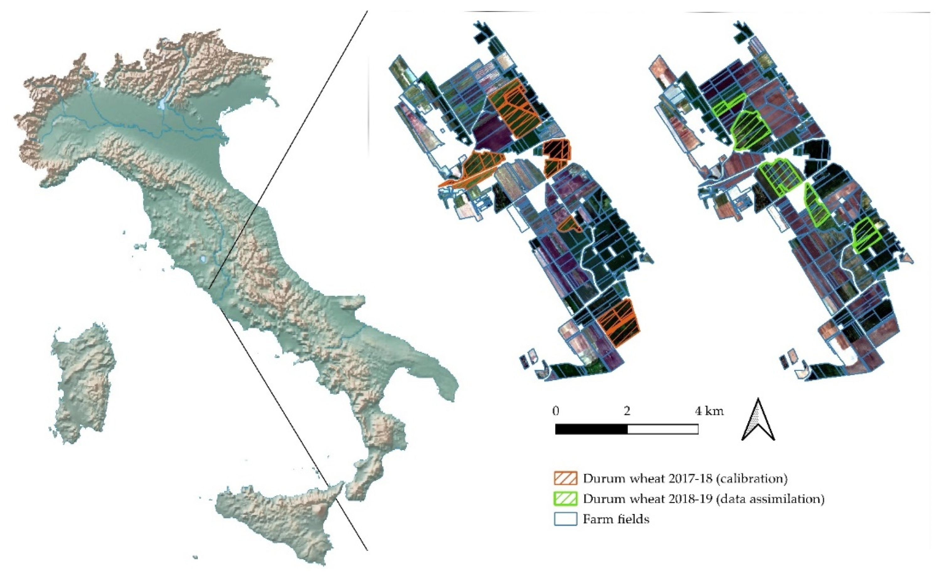
Figure 1. Maccarese farm area and durum wheat fields’ locations. Durum wheat fields of the 2017–2018 growing season were used for calibration, whereas durum wheat fields of the 2018–2019 growing season for data assimilation. RGB Sentinel-2 images (https://scihub.copernicus.eu/ accessed on 13 April 2020) of 6 April 2018 and 22 March 2019 were used as a base layer for the field.
Remotesensing 13 02889 g001
Figure 2. Study areas in New Zealand: Takaka region (A)-Te Puke region (B), and in Italy: Cisterna di Latina (C).
Remotesensing 13 02889 g002
Figure 3. Infected and not-infected digitalized blocks in the Te Puke region (A) and in the Takaka region (New Zealand) (B).
Remotesensing 13 02889 g003
Figure 4. Acquisition of hyperspectral images of leaves (a) and the method and result of wheat yellow rust identification (b).
Remotesensing 13 02889 g004
Figure 5. Acquisition of UAV hyperspectral images (a), and extraction of wavelet features and results of wheat yellow rust monitoring (b).
Remotesensing 13 02889 g005
Figure 6. A false color map of the research area and survey area of Ningqiang, Shaanxi Province; the wheat planting area is shown in green, and the sampling points are marked yellow.
Remotesensing 13 02889 g006
Figure 7. Data assimilation of LAI retrieved from Sentinel 2 into SAFYsw model. For each durum wheat field (ag), the graphs represent the LAI curve fitted on Sentinel-2, the LAI simulated without data assimilation (open loop) and the LAI simulated with data assimilation (see legend in panel h)). EO-derived LAI curves and LAI curves simulated with data assimilation overlaps.
Remotesensing 13 02889 g007
Figure 8. Simulated yield (with data assimilation) vs. observed yield.
Remotesensing 13 02889 g008
Figure 9. ROC Curves showing the performance of the classificatory when applied to RapidEye images. Class 1 indicates infected blocks, while class 2 indicates blocks where the pest has not been detected.
Remotesensing 13 02889 g009
Figure 10. Results of the application of the trained NN on kiwi fields in Italy. The legend shows the probability of a field infection (in this case, representing similar behavior as those fields validated in other regions of interest).
Remotesensing 13 02889 g010
Figure 11. Monitoring and mapping of yellow rust and ground truth maps in Ningqiang County, Shaanxi Province (China). The window shows an enlarged view of the stripe rust distribution in the sub-area.
Remotesensing 13 02889 g011
Table 1. List of SAFYsw parameters and values used in the simulations.
ParameterMeaningMeanRange 1Source
Crop growth parameters
εCClimatic efficiency0.48 [13,17]
εlLight interception coefficient0.5 [13,17]
SLASpecific leaf area (m2·g−1)0.22 [13,17]
ToptOptimum temperature for development (°C)20 [13,17]
TminMinimum temperature for development (°C)0 [13,17]
TmaxMaximum temperature for development (°C)37 [13,17]
DAM0Initial dry aboveground biomass (g·m−2)4.55 LAI/SLA with LAI = 0.1 [13,17]
D0Emergence date (day of year)354 Varies on visual inspection of LAI curve
ELUEEffective light use efficiency (g·MJ−1)3.452.9–4.0Calibrated
PyPartition to grain (grain filling rate)0.00490.0028–0.007Calibrated
Phenology parameters
PLaParameter A of partition to leaf0.1210.067–0.175Calibrated
PLbParameter B of partition to leaf0.00250.002–0.003Calibrated
STTGrowing degree days (GDD) to senescence1225850–1600Calibrated
RSRate of senescence (GDD·day−1)20,5008000–33,000Calibrated
Soil parameters
RootRatioRoot weight to length ratio (cm·g−1)0.98 [41]
RtGrtRateRoot growth rate (cm·GDD−1)0.22 [41]
MxRDPMaximum root depth (cm)120 [41]
RnffRunoff factor (ratio to total rainfall)0.15 [41]
SALBSoil albedo0.16 [41]
SWCONProfile drainage coefficient (soil water conductivity)0.90 [41]
MxRWUMax root water uptake (cm3 water·cm−1 root)0.0035 [41]
SATSaturation water content (cm3·cm−3)0.479 Pedotransfer from ESDAC–JRC soil maps.
Differences of values for the same soil water limit across fields were minimal (< 0.03 cm3·cm−3)
DULDrained upper limit (cm3·cm−3)0.240
LLLower limit (cm3·cm−3)0.115
AirDryResidual humidity (cm3·cm−3)0.055
1 For calibration and data assimilation.
Table 2. Performance metrics of yield estimations for 2019 with and without data assimilation. RMSE (root mean square error) and MAE (mean absolute value) are in tons per hectare, RRMSE (relative RMSE) is in percentage. Metrics are obtained by comparing predicted and observed yield for each field.
SimulationRMSE t·ha−1RRMSE %MAE %
With data assimilation1.4231.71.14
Open loop4.4297.33.97
Table 3. Confusion matrix results from the application of the NN classification on RapidEye VI.
Training Confusion MatrixValidation Confusion Matrix
Output class 136.3%3.8%90.6%25.0%8.8%74.1%
Output class 25.4%54.6%91.0%5
6.3%
48
60.0%
90.6%
87.0%93.6%85.0%80.0%87.3%85.0%
Target class 1Target class 2AOTarget class 1Target class 2AO
Test Confusion MatrixAll Confusion Matrix
Output class 122.5%10.0%69.2%31.3%6.0%83.9%
Output class 25.0%62.5%92.6%5.5%57.3%91.2%
81.8%86.2%85.0%85.0%90.5%88.5%
Target class 1Target class 2AOTarget class 1Target class 2AO
Table 4. Confusion matrix result from the application of the NN classification procedure with the new dataset.
Training Confusion MatrixValidation Confusion Matrix
Output class 159.5%5.4%91.7%61.5%5.4%92.0%
Output class 22.1%33.1%94.2%5.4%27.7%83.7%
96.7%86.0%92.6%92.0%83.7%89.2%
Target class 1Target class 2OATarget class 1Target class 2OA
Test Confusion MatrixAll Confusion Matrix
Output class 152.3%2.3%95.8%31.3%6.0%83.9%
Output class 23.8%41.5%91.5%5.5%57.3%91.2%
93.2%94.7%93.8%85.0%90.5%88.5%
Target class 1Target class 2OATarget class 1Target class 2OA
Table 5. Performance of the classifier with the new set of VIs.
Training Confusion MatrixValidation Confusion Matrix
Output class 158.5%5.4%95.8%63.1%1.5%97.6%
Output class 22.3%36.7%94.1%0.0%35.4%100%
96.2%93.5%95.1%100.0%95.8%98.5%
Target class 1Target class 2OATarget class 1Target class 2OA
Test Confusion MatrixAll Confusion Matrix
Output class 160.0%3.1%95.1%59.7%2.5%96.0%
Output class 22.3%34.6%93.8%1.8%36.0%95.1%
96.3%91.8%94.6%97.0%93.6%95.7%
Target class 1Target class 2OATarget class 1Target class 2OA
Table 6. Comparison between confusion matrices.
Confusion Matrix with 12 Initial VIsConfusion Matrix with Extended List of VIs
Output class 158.5%4.8%59.7%2.5%
Output class 23.1%33.7%1.8%36.0%
Target class 1Target class 2Target class 1Target class 2
Table 7. Results obtained from the application of the neural network, trained with VIs computed on PRISMA images, on the two regions in New Zealand. As in the previous cases, the characteristics of the neural network included 60% of the samples for training, 20% for validation, and 20% for testing, with 20 hidden neurons.
Confusion Matrix with 12 Initial VIs
Output class 158.5%4.8%92.5%
Output class 23.1%33.7%91.6%
95%87.6%92.2%
Confusion Matrix with Extended List of VIs
Output class 159.7%2.5%96.0%
Output class 21.6%36.0%95.1%
97%93.6%95.7%
Target class 1Target class 2OA
Table 8. Changes in average monitoring accuracy of yellow rust monitoring model after infestation, expressed in days after infection (DAI).
FeatureClassClassification Accuracy (%)
7 DAI14 DAI21 DAI28 DAI31 DAI34 DAI41 DAI
WRSFsHealthy73.581.288.695.496.995.296.1
Infected80.584.879.892.798.298.498.5
Table 9. Monitoring accuracy of KPCA-SVM based on UAV hyperspectral imagery, at different days after infection (DAI).
ModelStateClassification Accuracy/%
7 DAI14 DAI21 DAI28 DAI31 DAI34 DAI41 DAI
KPCA-SVMHealthy88.792.497.599.298.896.798.9
Infected84.290.195.397.910010098.2
Table 10. Confusion matrix and kappa value for the monitoring results based on KPCA-SVM of the yellow rust in Ningqiang county (China).
Healthy
Wheat
Yellow
Rust
User’s
Accuracy (%)
Overall
Accuracy (%)
Kappa Coefficient
Healthy wheat1648084.60.742
Yellow rust21789.5
Producer’s accuracy (%)88.981
Publisher’s Note: MDPI stays neutral with regard to jurisdictional claims in published maps and institutional affiliations.