
Sino–EU Earth Observation Data to Support the Monitoring and Management of Agricultural Resources

 ,
,  ,
,  , ,
, ,  ,
,  ,
,  , ,
, , 
Abstract
: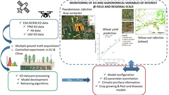
1. Introduction
2. Materials and Methods
2.1. Retrieval of Biophysical and Agronomical Variables
2.1.1. Coupling EO Data with Crop Models for Yield Prediction
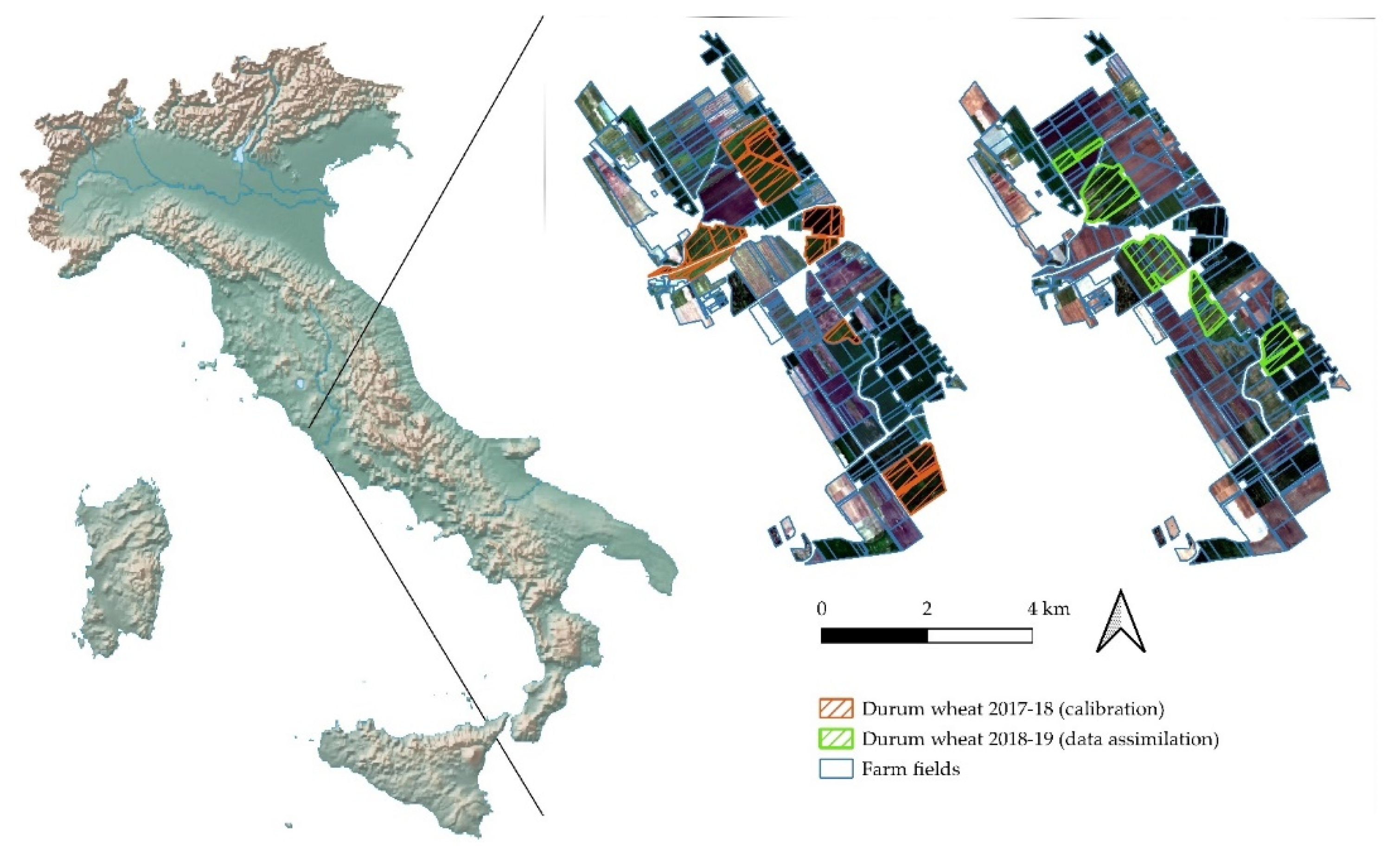
2.1.2. Cropping Seasons and Input Variables
- A spline interpolation was used to fill the missing dates with LAI values to ensure continuous data throughout the entire growing season.
- A 4253H twice filter was used as a form of moving average to smooth LAI values.
- A double logistic curve was fit to provide a more realistic representation of the field-wise LAI curves. LAI fit following [29,30,31] were visually inspected to select the best fitting method that gave the most realistic LAI curves given the satellite data available. The equation reported by [31] was finally selected.
2.1.3. SAFYsw Model Calibration and Data Assimilation
2.2. Crop Diseases Detection Methods
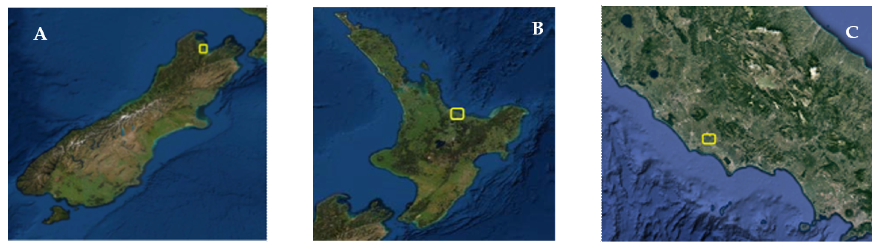
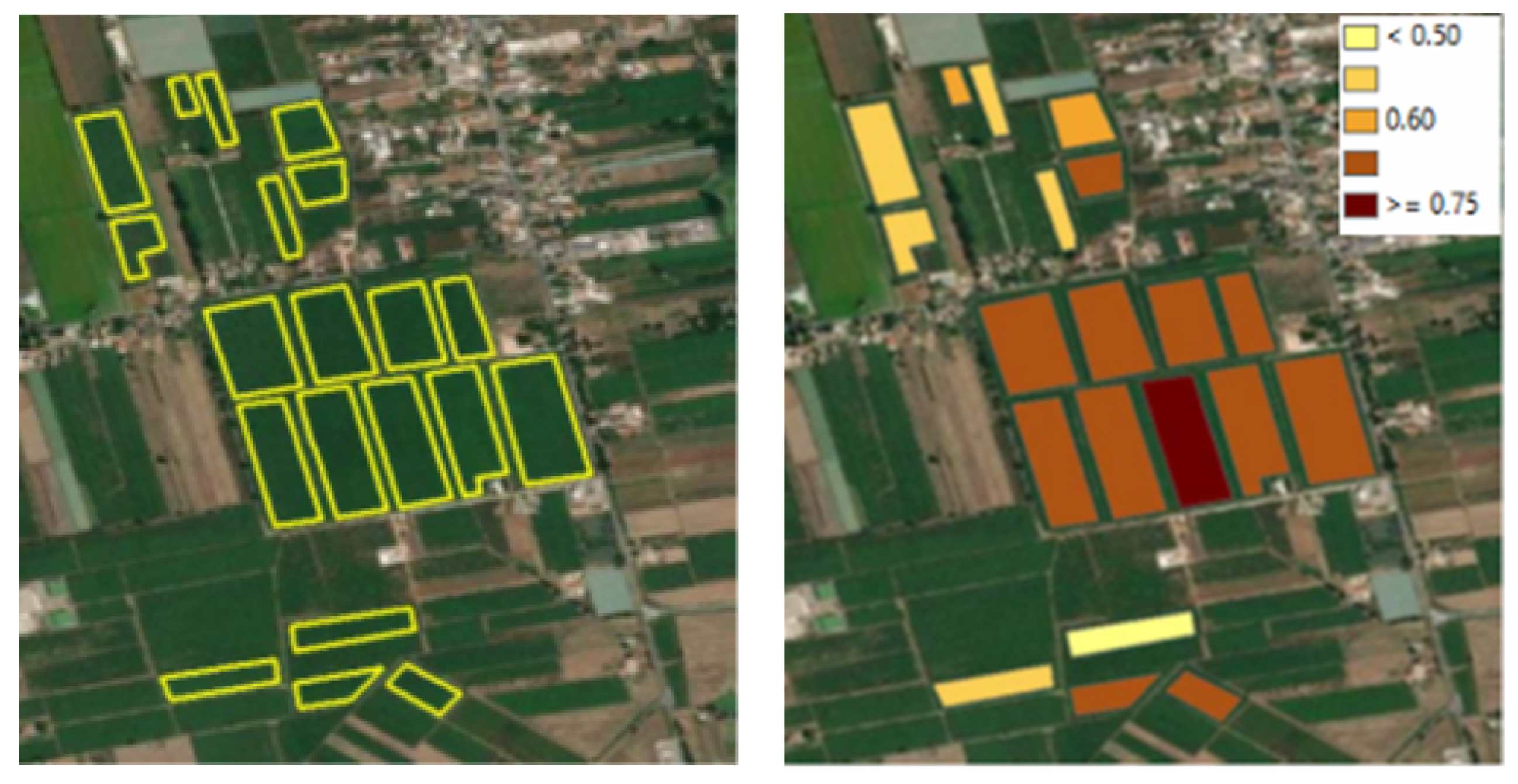
2.2.1. Orchards Diseases Detection
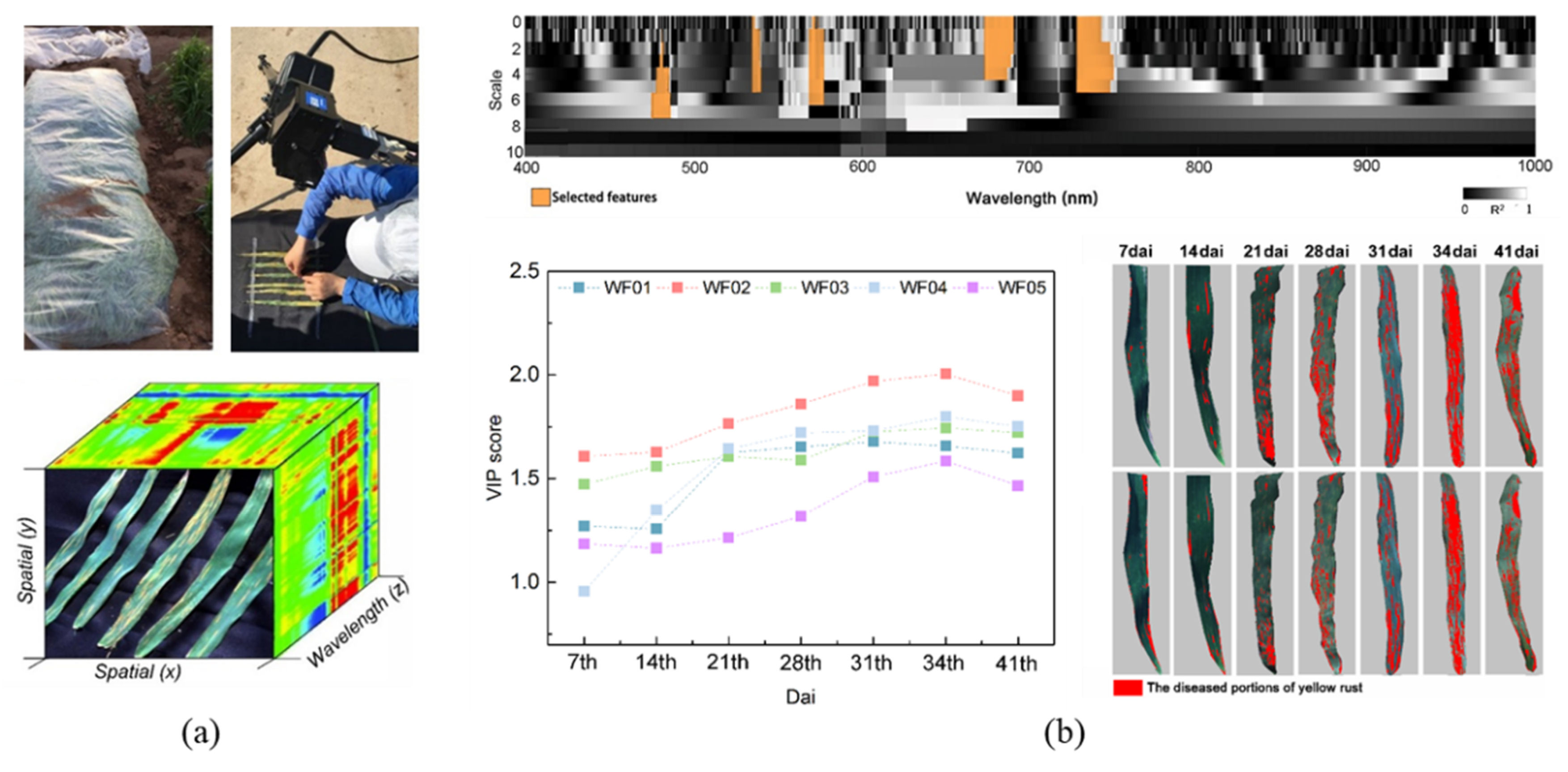
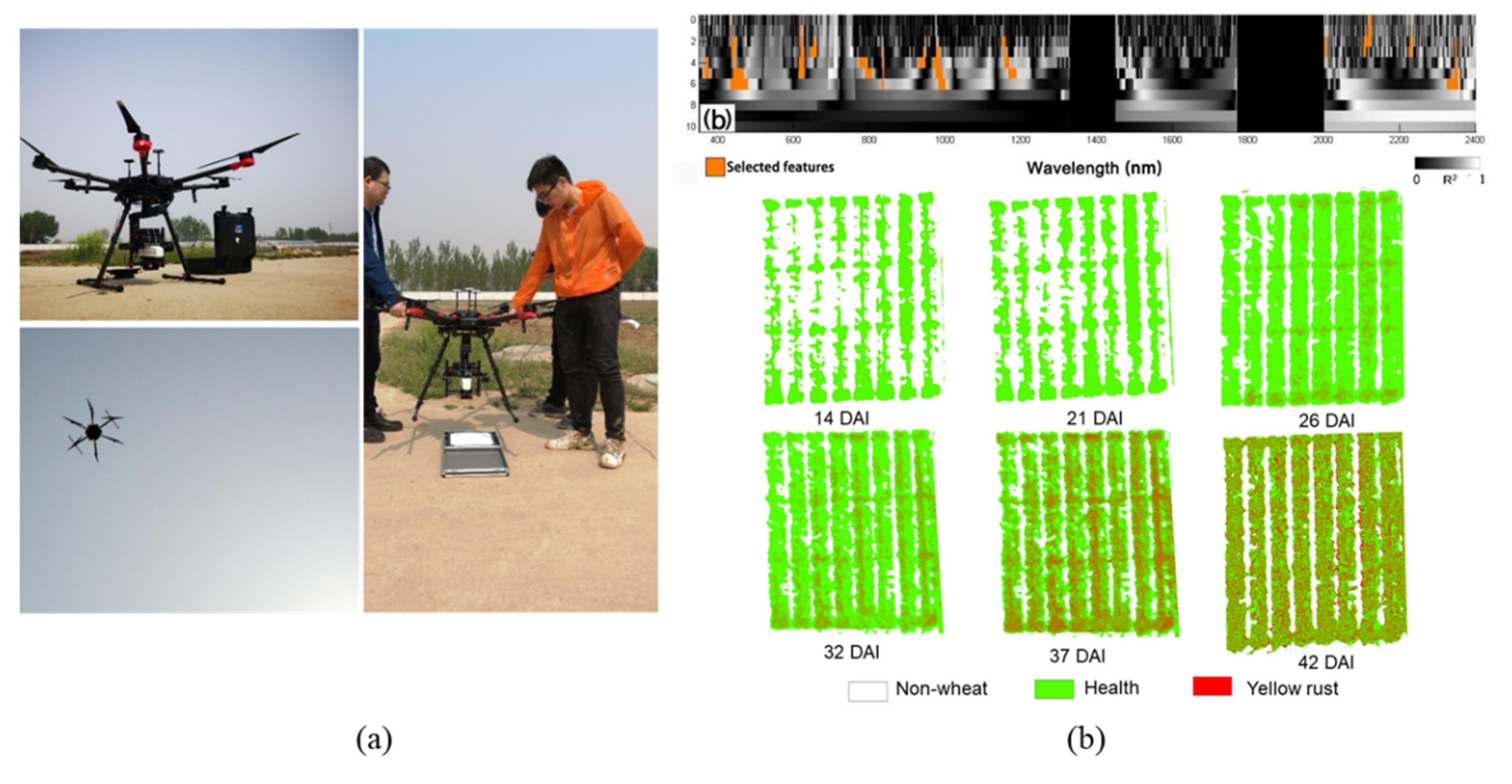
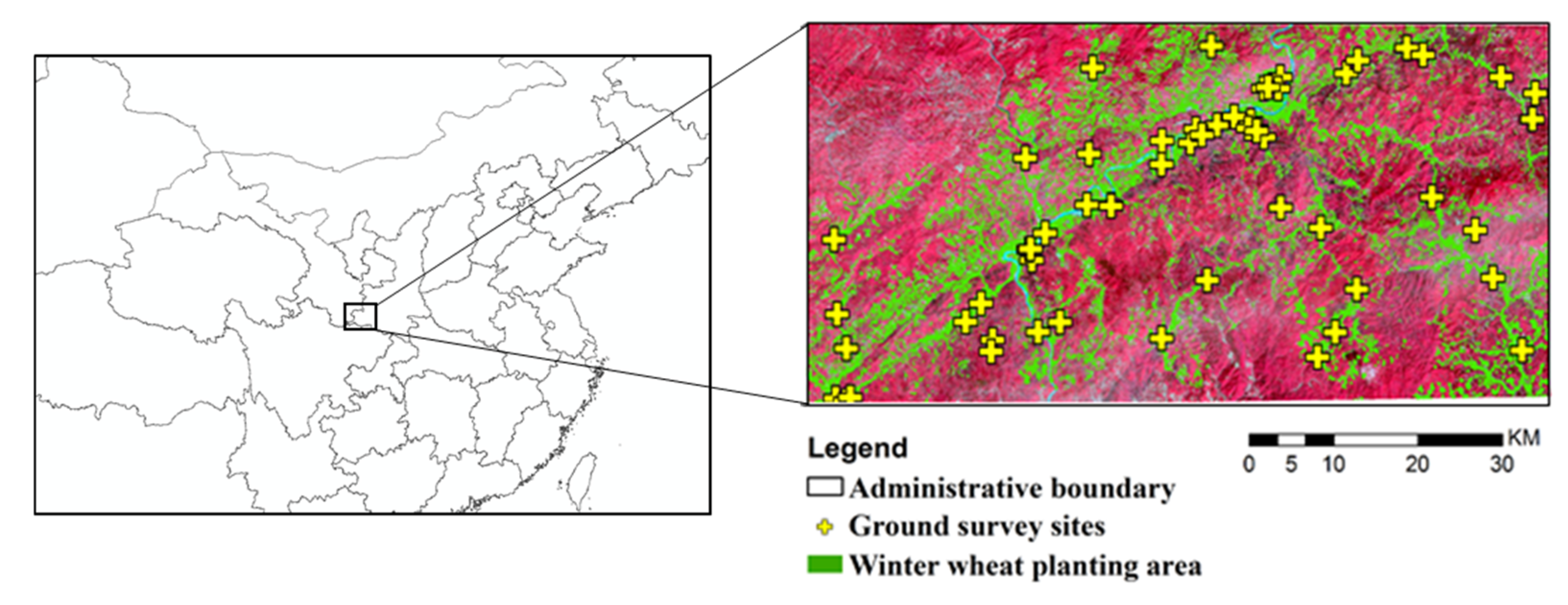
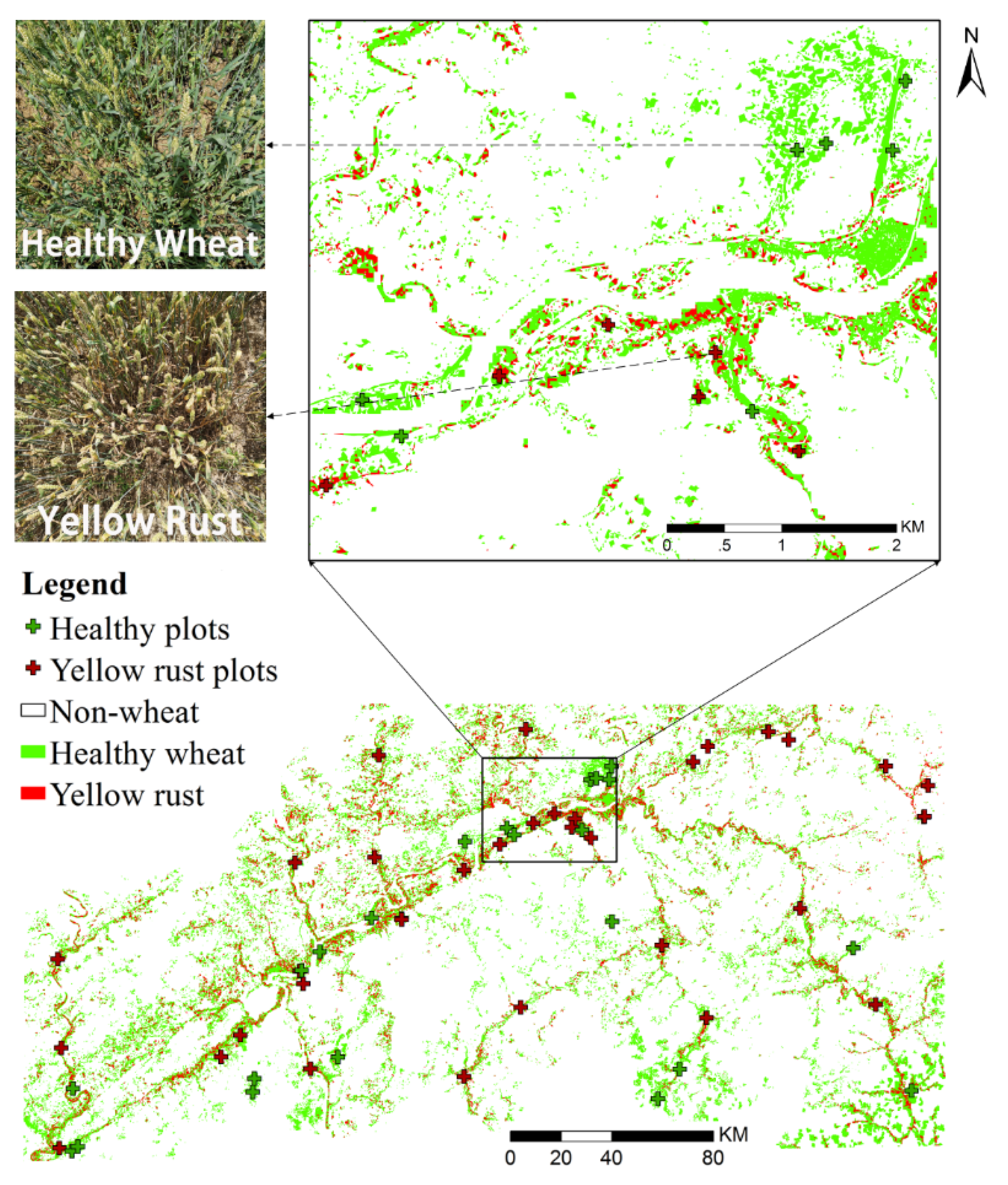
2.2.2. Wheat Yellow Rust Detection
3. Results
3.1. Coupling EO Data with Crop Models for Yield Prediction
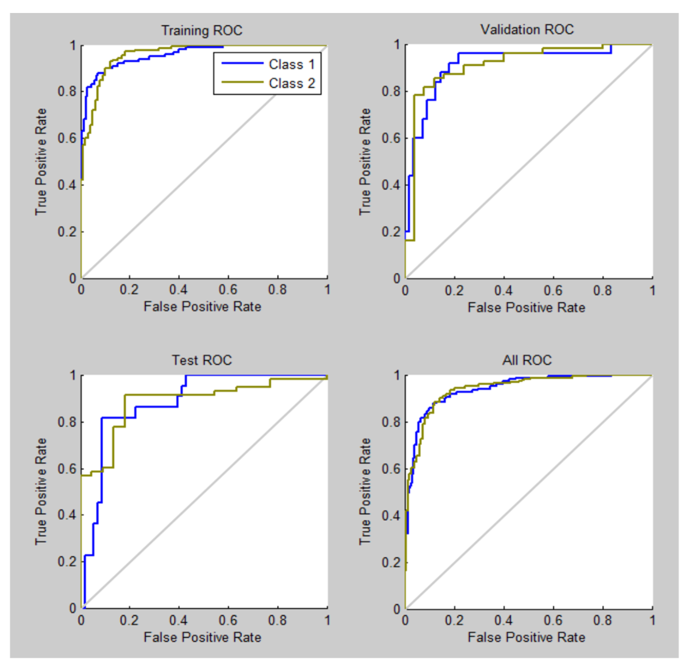
3.2. Crop Diseases Results
3.2.1. Orchards Diseases Mapping
3.2.2. Wheat Yellow Rust Mapping
4. Discussion
5. Conclusions
- (a)
- Expand the estimation of new variables, by exploring the RTM code PROSPECT-PRO (e.g., for proteins and nitrogen);
- (b)
- Exploit the newly operative hyperspectral missions for their application on a regional base to detect pathogens;
- (c)
- The implementation of machine/deep learning techniques for the generalization of the pre-operative chains applicable to the local scale for agricultural applications.
Author Contributions
Funding
Institutional Review Board Statement
Informed Consent Statement
Data Availability Statement
Acknowledgments
Conflicts of Interest
Appendix A. Simple Algorithm for Yield Estimates (SAFY)
Appendix B. The Ensemble Kalman Filter (EnKF) Assimilation Procedure
- Initialization of the model ensemble: an ensemble of N model simulations (N = 100 in our case) was generated. Each element of the ensemble was obtained by creating a different set of model parameters. Some parameters were considered fixed (Table 1), while for the calibrated parameters a value was randomly sampled from a truncated gaussian distribution with fixed average and lower and upper limits corresponding to the range obtained during the calibration (Table 1). This perturbation allows for the simulation of the error covariance.
- Forecast step: a simulation was run with a daily timestep separately for each element of the model ensemble, till the day of observation, to obtain an ensemble of simulated LAI values. The error covariance of the forecast can be calculated from the ensemble as in Equation (A12):where (PE)tf is the error covariance of the ensemble of forecasts at time t, E|Xt| the ensemble of model state variables (LAI in this case) at time t, and Xt is the simulated LAI mean value.(PE)tf = (Xt − E|Xt|)∙(Xt − E|Xt|)T/(N − 1),
- Observation error propagation: an ensemble of N LAI observations was generated for each day with a LAI observation (in our case, each day of the growth cycle, due to the LAI fitting procedure). The ensemble was obtained by randomly sampling from a gaussian distribution with an average equal to the EO-derived LAI value and a standard deviation of 10%. Similarly, to the simulated values, the error covariance of the observation can be calculated from the ensemble as in Equation (A13):where (RE)tf is the error covariance of the ensemble of observations at time t, E|Yt| the ensemble of observations and Yt the original mean value.(RE)tf = (Yt − E|Yt|)∙(Yt − E|Yt|)T/(N − 1),
- Update step: the mean state and the model state covariances are updated using the Kalman gain (for each ensemble element) following Equation (A14):where Kt is the Kalman gain at time t, Ptf is the model state forecast at time t, H is the observation operator, assumed constant over time, Rt is the measurement error at time t.Kt = Ptf∙HT∙(H∙Ptf∙HT + Rt)−1,The mean state was (Equation (A15)):where xta is the updated mean state, obtained from the combination of the model forecast mean state xtf, the observation mean xtf, and the Kalman gain.xta = xtf + Kt∙(yt − Hxtf),The model state covariance at time t (Pta) is expressed by Equation (A16):where I is the identity matrix.Pta = (I − Kt∙H)∙Ptf,
- The forecast, observation error propagation and update steps were repeated recursively till the end of the simulation, assimilating each new observation.
References
- Jia, K.; Wu, B.; Li, Q. Crop classification using HJ satellite multispectral data in the North China Plain. J. Appl. Remote Sens. 2013, 7, 073576. [Google Scholar] [CrossRef]
- Whitcraft, A.K.; Becker-Reshef, I.; Killough, B.D.; Justice, C.O. Meeting earth observation requirements for global agricultural monitoring: An evaluation of the revisit capabilities of current and planned moderate resolution optical earth observing missions. Remote Sens. 2015, 7, 1482–1503. [Google Scholar] [CrossRef] [Green Version]
- Ozdarici-Ok, A.; Ok, A.O.; Schindler, K. Mapping of agricultural crops from single high-resolution multispectral images—Data-driven smoothing vs. parcel-based smoothing. Remote Sens. 2015, 7, 5611–5638. [Google Scholar] [CrossRef] [Green Version]
- Zhou, T.; Pan, J.; Zhang, P.; Wei, S.; Han, T. Mapping Winter Wheat with Multi-Temporal SAR and Optical Images in an Urban Agricultural Region. Sensors 2017, 17, 1210. [Google Scholar] [CrossRef] [PubMed]
- Veloso, A.; Mermoz, S.; Bouvet, A.; Le Toan, T.; Planells, M.; Dejoux, J.F.; Ceschia, E. Understanding the temporal behavior of crops using Sentinel-1 and Sentinel-2-like data for agricultural applications. Remote Sens. Environ. 2017, 199, 415–426. [Google Scholar] [CrossRef]
- Brook, A.; De Micco, V.; Battipaglia, G.; Erbaggio, A.; Ludeno, G.; Catapano, I.; Bonfante, A. A smart multiple spatial and temporal resolution system to support precision agriculture from satellite images: Proof of concept on Aglianico vineyard. Remote Sens. Environ. 2020, 240, 111679. [Google Scholar] [CrossRef]
- Zhang, L.; Zhang, Z.; Luo, Y.; Cao, J.; Tao, F. Combining Optical, Fluorescence, Thermal Satellite, and Environmental Data to Predict County-Level Maize Yield in China Using Machine Learning Approaches. Remote Sens. 2019, 12, 21. [Google Scholar] [CrossRef] [Green Version]
- Zhao, L.; Huang, W.; Chen, J.; Dong, Y.; Ren, B.; Geng, Y. Land use/cover changes in the Oriental migratory locust area of China: Implications for ecological control and monitoring of locust area. Agric. Ecosyst. Environ. 2020, 303, 107110. [Google Scholar] [CrossRef]
- Zhou, X.; Zhang, J.; Chen, D.; Huang, Y.; Kong, W.; Yuan, L.; Ye, H.; Huang, W. Assessment of Leaf Chlorophyll Content Models for Winter Wheat Using Landsat-8 Multispectral Remote Sensing Data. Remote Sens. 2020, 12, 2574. [Google Scholar] [CrossRef]
- Weiss, M.; Jacob, F.; Duveiller, G. Remote sensing for agricultural applications: A meta-review. Remote Sens. Environ. 2020, 236, 111402. [Google Scholar] [CrossRef]
- Silvestro, P.C.; Pignatti, S.; Pascucci, S.; Yang, H.; Li, Z.; Yang, G.; Huang, W.; Casa, R. Estimating Wheat Yield in China at the Field and District Scale from the Assimilation of Satellite Data into the Aquacrop and Simple Algorithm for Yield (SAFY) Models. Remote Sens. 2017, 9, 509. [Google Scholar] [CrossRef] [Green Version]
- Guo, C.; Tang, Y.; Lu, J.; Zhu, Y.; Cao, W.; Cheng, T.; Zhang, L.; Tian, Y. Predicting wheat productivity: Integrating time series of vegetation indices into crop modeling via sequential assimilation. Agric. For. Meteorol. 2019, 272, 69–80. [Google Scholar] [CrossRef]
- Duchemin, B.; Maisongrande, P.; Boulet, G.; Benhadj, I. A simple algorithm for yield estimates: Evaluation for semi-arid irrigated winter wheat monitored with green leaf area index. Environ. Model. Softw. 2008, 23, 876–892. [Google Scholar] [CrossRef] [Green Version]
- Upreti, D.; Pignatti, S.; Pascucci, S.; Tolomio, M.; Li, Z.; Huang, W.; Casa, R. A Comparison of Moment-Independent and Variance-Based Global Sensitivity Analysis Approaches for Wheat Yield Estimation with the Aquacrop-OS Model. Agronomy 2020, 10, 607. [Google Scholar] [CrossRef]
- Upreti, D.; Pignatti, S.; Pascucci, S.; Tolomio, M.; Huang, W.; Casa, R. Bayesian Calibration of the Aquacrop-OS Model for Durum Wheat by Assimilation of Canopy Cover Retrieved from VENµS Satellite Data. Remote Sens. 2020, 12, 2666. [Google Scholar] [CrossRef]
- Li, Z.; Taylor, J.; Yang, H.; Casa, R.; Jin, X.; Li, Z.; Song, X.; Yang, G. A hierarchical interannual wheat yield and grain protein prediction model using spectral vegetative indices and meteorological data. Field Crop. Res. 2020, 248, 107711. [Google Scholar] [CrossRef]
- Dong, Y.; Xu, F.; Liu, L.; Du, X.; Ren, B.; Guo, A.; Geng, Y.; Ruan, C.; Ye, H.; Huang, W.; et al. Automatic System for Crop Pest and Disease Dynamic Monitoring and Early Forecasting. IEEE J. Sel. Top. Appl. Earth Obs. Remote. Sens. 2020, 13, 4410–4418. [Google Scholar] [CrossRef]
- Guo, A.; Huang, W.; Ye, H.; Dong, Y.; Ma, H.; Ren, Y.; Ruan, C. Identification of Wheat Yellow Rust Using Spectral and Texture Features of Hyperspectral Images. Remote Sens. 2020, 12, 1419. [Google Scholar] [CrossRef]
- Ma, H.; Huang, W.; Jing, Y.; Pignatti, S.; Laneve, G.; Dong, Y.; Ye, H.; Liu, L.; Guo, A.; Jiang, J. Identification of Fusarium Head Blight in Winter Wheat Ears Using Continuous Wavelet Analysis. Sensors 2019, 20, 20. [Google Scholar] [CrossRef] [Green Version]
- Liu, L.; Dong, Y.; Huang, W.; Du, X.; Ma, H. Monitoring Wheat Fusarium Head Blight Using Unmanned Aerial Vehicle Hyperspectral Imagery. Remote Sens. 2020, 12, 3811. [Google Scholar] [CrossRef]
- Loizzo, R.; Guarini, R.; Longo, F.; Scopa, T.; Formaro, R.; Facchinetti, C.; Varacalli, G. Prisma: The Italian Hyperspectral Mission. In Proceedings of the IGARSS 2018-2018 IEEE International Geoscience and Remote Sensing Symposium, Valencia, Spain, 22–27 July 2018; pp. 175–178. [Google Scholar]
- Ren, K.; Sun, W.; Meng, X.; Yang, G.; Du, Q. Fusing China GF-5 Hyperspectral Data with GF-1, GF-2 and Sentinel-2A Multispectral Data: Which Methods Should Be Used? Remote Sens. 2020, 12, 882. [Google Scholar] [CrossRef] [Green Version]
- Matsunaga, T.; Iwasaki, A.; Tsuchida, S.; Iwao, K.; Tanii, J.; Kashimura, O.; Nakamura, R.; Yamamoto, H.; Kato, S.; Obata, K.; et al. Current status of Hyperspectral Imager Suite (HISUI) onboard International Space Station (ISS). In Proceedings of the 2017 IEEE International Geoscience and Remote Sensing Symposium (IGARSS), Fort Worth, TX, USA, 23–28 July 2017; pp. 443–446. [Google Scholar]
- Mahalingam, S.; Srinivas, P.; Devi, P.K.; Sita, D.; Das, S.K.; Leela, T.S.; Venkataraman, V.R. Reflectance based vicarious calibration of HySIS sensors and spectral stability study over pseudo-invariant sites. In Proceedings of the IEEE Recent Advances in Geoscience and Remote Sensing: Technologies, Standards and Applications (TENGARSS), Grand Hyatt Kochi Bolgatti, Kerala, India, 17–20 October 2019; pp. 132–136. [Google Scholar]
- Alonso, K.; Bachmann, M.; Burch, K.; Carmona, E.; Cerra, D.; Reyes, R.D.L.; Dietrich, D.; Heiden, U.; Hölderlin, A.; Ickes, J.; et al. Data Products, Quality and Validation of the DLR Earth Sensing Imaging Spectrometer (DESIS). Sensors 2019, 19, 4471. [Google Scholar] [CrossRef] [PubMed] [Green Version]
- Guanter, L.; Kaufmann, H.; Segl, K.; Foerster, S.; Rogass, C.; Chabrillat, S.; Hollstein, A.; Rossner, G.; Chlebek, C.; Sang, B.; et al. The EnMAP spaceborne imaging spectroscopy mission for earth observation. Remote Sens. 2015, 7, 8830–8857. [Google Scholar] [CrossRef] [Green Version]
- Boccia, V.; Adams, J.; Thome, K.J.; Turpie, K.R.; Kokaly, R.; Bouvet, M.; Green, R.O.; Rast, M. NASA-ESA Cooperation on the SBG and CHIME Hyperspectral Satellite Missions: A roadmap for the joint Working Group on Cal/Val activities (No. EGU21-15166). In EGU General Assembly Conference Abstracts; The European Geosciences Union: San Francisco, CA, USA, 2021. [Google Scholar]
- Zeng, L.; Wardlow, B.D.; Xiang, D.; Hu, S.; Li, D. A review of vegetation phenological metrics extraction using time-series, multispectral satellite data. Remote Sens. Environ. 2020, 237, 111511. [Google Scholar] [CrossRef]
- Beck, P.S.; Atzberger, C.; Høgda, K.A.; Johansen, B.; Skidmore, A.K. Improved monitoring of vegetation dynamics at very high latitudes: A new method using MODIS NDVI. Remote Sens. Environ. 2006, 100, 321–334. [Google Scholar] [CrossRef]
- Elmore, A.J.; Guinn, S.M.; Minsley, B.J.; Richardson, A.D. Landscape controls on the timing of spring, autumn, and growing season length in mid-Atlantic forests. Glob. Change Biol. 2012, 18, 656–674. [Google Scholar] [CrossRef] [Green Version]
- Gu, L.; Post, W.M.; Baldocchi, D.D.; Black, T.A.; Suyker, A.E.; Verma, S.B.; Vesala, T.; Wofsy, S.C. Characterizing the seasonal dynamics of plant community photosynthesis across a range of vegetation types. In Phenology of Ecosystem Processes; Noormets, A., Ed.; Springer: New York, NY, USA, 2009; pp. 35–58. [Google Scholar]
- Ballabio, C.; Panagos, P.; Monatanarella, L. Mapping topsoil physical properties at European scale using the LUCAS database. Geoderma 2016, 261, 110–123. [Google Scholar] [CrossRef]
- Ritchie, J.T.; Gerakis, A.; Suleiman, A. Simple model to estimate field-measured soil water limits. Trans. ASAE 1999, 42, 1609. [Google Scholar] [CrossRef]
- Jones, J.W.; Hoogenboom, G.; Porter, C.H.; Boote, K.J.; Batchelor, W.D.; Hunt, L.A.; Wilkens, P.A.; Singh, P.; Gijsman, A.J.; Ritchie, J.T. The DSSAT cropping system model. Eur. J. Agron. 2003, 18, 235–265. [Google Scholar] [CrossRef]
- Monteith, J.L. Solar radiation and productivity in tropical ecosystems. J. Appl. Ecol. 1972, 9, 747–766. [Google Scholar] [CrossRef] [Green Version]
- Monteith, J.L. Climate and the efficiency of crop production in Britain. Philos. Trans. R. Soc. Lond. B Biol. Sci. 1977, 281, 277–294. [Google Scholar]
- Trudgill, D.L.; Honek, A.; Li, D.; Van Straalen, N.M. Thermal time—Concepts and utility. Ann. Appl. Biol. 2005, 146, 1–14. [Google Scholar] [CrossRef]
- Wallach, D.; Makowski, D.; Jones, J.W.; Brun, F. Working with Dynamic Crop Models: Methods, Tools and Examples for Agriculture and Environment, 2nd ed.; Academic Press: London, UK, 2014; ISBN 978-0-12-397008-4. [Google Scholar]
- Kalman, R.E. A new approach to linear filtering and prediction problems. J. Basic Eng. 1960, 82, 35–45. [Google Scholar] [CrossRef] [Green Version]
- The MathWorks, Inc, MATLAB (Version R2019b, Academic Use). 2019. Available online: https://www.mathworks.com/ (accessed on 1 April 2021).
- Kang, Y.; Özdoğan, M. Field-level crop yield mapping with Landsat using a hierarchical data assimilation approach. Remote Sens. Environ. 2019, 228, 144–163. [Google Scholar] [CrossRef]
- Greer, G.; Saunders, C. The costs of Psa-V to the New Zealand Kiwifruit Industry and the Wider Community; Agribusiness and Economics Research Unit 62: Lincoln, New Zealand, 2012. [Google Scholar]
- Laneve, G.; Luciani, R.; Marzialetti, P.; Pignatti, S.; Huang, W.; Shi, Y.; Dong, Y.; Ye, H. Dragon 4—Satellite based analysis of diseases on permanent and row crops in Italy and China. J. Geod. Geoinf. Sci. 2020, 3, 107–118. [Google Scholar]
- Vanneste, J.L.; Giovanardi, D.; Yu, J.; Cornish, D.A.; Kay, C.; Spinelli, F.; Stefani, E. Detection of Pseudomonas syringae pv. actinidiae in kiwifruit pollen samples. N. Z. Plant Prot. 2011, 64, 246–251. [Google Scholar] [CrossRef] [Green Version]
- Taylor, J.A.; Mowat, A.D.; Bollen, A.F.; Whelan, B.M. Early season detection and mapping of Pseudomonas syringae pv. actinidae infected kiwifruit (Actinidia sp.) orchards. N. Z. J. Crop Hortic. Sci. 2014, 42, 303–311. [Google Scholar] [CrossRef] [Green Version]
- ProMed Posting (no. 20110822.2550). Bacterial Canker, Kiwifruit—New Zealand, Italy: Spread. Available online: www.promedmail.org (accessed on 22 August 2011).
- Palmieri, A.; Pirazzoli, C. L’actinidia in Italia e nel mondo tra concorrenza e nuove opportunità. Riv. Fruttic. 2014, 12, 66–68. [Google Scholar]
- Nawar, S.; Corstanje, R.; Halcro, G.; Mulla, D.; Mouazen, A.M. Delineation of soil management zones for variable-rate fertilization: A review. Adv. Agron. 2017, 143, 175–245. [Google Scholar]
- Peng, X.; Han, W.; Ao, J.; Wang, Y. Assimilation of LAI Derived from UAV Multispectral Data into the SAFY Model to Estimate Maize Yield. Remote Sens. 2021, 13, 1094. [Google Scholar] [CrossRef]
- Kasampalis, D.A.; Alexandridis, T.K.; Deva, C.; Challinor, A.; Moshou, D.; Zalidis, G. Contribution of remote sensing on crop models: A review. J. Imaging 2018, 4, 52. [Google Scholar] [CrossRef] [Green Version]
- Tolomio, M.; Casa, R. Dynamic Crop Models and Remote Sensing Irrigation Decision Support Systems: A Review of Water Stress Concepts for Improved Estimation of Water Requirements. Remote Sens. 2020, 12, 3945. [Google Scholar] [CrossRef]
- Pascucci, S.; Carfora, M.F.; Palombo, A.; Pignatti, S.; Casa, R.; Pepe, M.; Castaldi, F. A comparison between standard and functional clustering methodologies: Application to agricultural fields for yield pattern assessment. Remote Sens. 2018, 10, 585. [Google Scholar] [CrossRef] [Green Version]
- Basso, B.; Ritchie, J.T.; Cammarano, D.; Sartori, L. A strategic and tactical management approach to select optimal N fertilizer rates for wheat in a spatially variable field. Eur. J. Agron. 2011, 35, 215–222. [Google Scholar] [CrossRef]
- Fontanet, M.; Scudiero, E.; Skaggs, T.H.; Fernàndez-Garcia, D.; Ferrer, F.; Rodrigo, G.; Bellvert, J. Dynamic Management Zones for Irrigation Scheduling. Agric. Water Manag. 2020, 238, 106207. [Google Scholar] [CrossRef]
- Jin, X.; Kumar, L.; Li, Z.; Feng, H.; Xu, X.; Yang, G.; Wang, J. A review of data assimilation of remote sensing and crop models. Eur. J. Agron. 2018, 92, 141–152. [Google Scholar] [CrossRef]
- EFSA. Workshop on Xylella Fastidiosa; Knowledge Gaps and Research Priorities for the EU: 2016; John Wiley & Sons, Inc., European Distribution Centre: West Sussex, UK, 2016. [Google Scholar]


| Parameter | Meaning | Mean | Range 1 | Source |
|---|---|---|---|---|
| Crop growth parameters | ||||
| εC | Climatic efficiency | 0.48 | [13,17] | |
| εl | Light interception coefficient | 0.5 | [13,17] | |
| SLA | Specific leaf area (m2·g−1) | 0.22 | [13,17] | |
| Topt | Optimum temperature for development (°C) | 20 | [13,17] | |
| Tmin | Minimum temperature for development (°C) | 0 | [13,17] | |
| Tmax | Maximum temperature for development (°C) | 37 | [13,17] | |
| DAM0 | Initial dry aboveground biomass (g·m−2) | 4.55 | LAI/SLA with LAI = 0.1 [13,17] | |
| D0 | Emergence date (day of year) | 354 | Varies on visual inspection of LAI curve | |
| ELUE | Effective light use efficiency (g·MJ−1) | 3.45 | 2.9–4.0 | Calibrated |
| Py | Partition to grain (grain filling rate) | 0.0049 | 0.0028–0.007 | Calibrated |
| Phenology parameters | ||||
| PLa | Parameter A of partition to leaf | 0.121 | 0.067–0.175 | Calibrated |
| PLb | Parameter B of partition to leaf | 0.0025 | 0.002–0.003 | Calibrated |
| STT | Growing degree days (GDD) to senescence | 1225 | 850–1600 | Calibrated |
| RS | Rate of senescence (GDD·day−1) | 20,500 | 8000–33,000 | Calibrated |
| Soil parameters | ||||
| RootRatio | Root weight to length ratio (cm·g−1) | 0.98 | [41] | |
| RtGrtRate | Root growth rate (cm·GDD−1) | 0.22 | [41] | |
| MxRDP | Maximum root depth (cm) | 120 | [41] | |
| Rnff | Runoff factor (ratio to total rainfall) | 0.15 | [41] | |
| SALB | Soil albedo | 0.16 | [41] | |
| SWCON | Profile drainage coefficient (soil water conductivity) | 0.90 | [41] | |
| MxRWU | Max root water uptake (cm3 water·cm−1 root) | 0.0035 | [41] | |
| SAT | Saturation water content (cm3·cm−3) | 0.479 | Pedotransfer from ESDAC–JRC soil maps. Differences of values for the same soil water limit across fields were minimal (< 0.03 cm3·cm−3) | |
| DUL | Drained upper limit (cm3·cm−3) | 0.240 | ||
| LL | Lower limit (cm3·cm−3) | 0.115 | ||
| AirDry | Residual humidity (cm3·cm−3) | 0.055 | ||
| Simulation | RMSE t·ha−1 | RRMSE % | MAE % |
|---|---|---|---|
| With data assimilation | 1.42 | 31.7 | 1.14 |
| Open loop | 4.42 | 97.3 | 3.97 |
| Training Confusion Matrix | Validation Confusion Matrix | |||||
|---|---|---|---|---|---|---|
| Output class 1 | 36.3% | 3.8% | 90.6% | 25.0% | 8.8% | 74.1% |
| Output class 2 | 5.4% | 54.6% | 91.0% | 5 6.3% | 48 60.0% | 90.6% |
| 87.0% | 93.6% | 85.0% | 80.0% | 87.3% | 85.0% | |
| Target class 1 | Target class 2 | AO | Target class 1 | Target class 2 | AO | |
| Test Confusion Matrix | All Confusion Matrix | |||||
| Output class 1 | 22.5% | 10.0% | 69.2% | 31.3% | 6.0% | 83.9% |
| Output class 2 | 5.0% | 62.5% | 92.6% | 5.5% | 57.3% | 91.2% |
| 81.8% | 86.2% | 85.0% | 85.0% | 90.5% | 88.5% | |
| Target class 1 | Target class 2 | AO | Target class 1 | Target class 2 | AO | |
| Training Confusion Matrix | Validation Confusion Matrix | |||||
|---|---|---|---|---|---|---|
| Output class 1 | 59.5% | 5.4% | 91.7% | 61.5% | 5.4% | 92.0% |
| Output class 2 | 2.1% | 33.1% | 94.2% | 5.4% | 27.7% | 83.7% |
| 96.7% | 86.0% | 92.6% | 92.0% | 83.7% | 89.2% | |
| Target class 1 | Target class 2 | OA | Target class 1 | Target class 2 | OA | |
| Test Confusion Matrix | All Confusion Matrix | |||||
| Output class 1 | 52.3% | 2.3% | 95.8% | 31.3% | 6.0% | 83.9% |
| Output class 2 | 3.8% | 41.5% | 91.5% | 5.5% | 57.3% | 91.2% |
| 93.2% | 94.7% | 93.8% | 85.0% | 90.5% | 88.5% | |
| Target class 1 | Target class 2 | OA | Target class 1 | Target class 2 | OA | |
| Training Confusion Matrix | Validation Confusion Matrix | |||||
| Output class 1 | 58.5% | 5.4% | 95.8% | 63.1% | 1.5% | 97.6% |
| Output class 2 | 2.3% | 36.7% | 94.1% | 0.0% | 35.4% | 100% |
| 96.2% | 93.5% | 95.1% | 100.0% | 95.8% | 98.5% | |
| Target class 1 | Target class 2 | OA | Target class 1 | Target class 2 | OA | |
| Test Confusion Matrix | All Confusion Matrix | |||||
| Output class 1 | 60.0% | 3.1% | 95.1% | 59.7% | 2.5% | 96.0% |
| Output class 2 | 2.3% | 34.6% | 93.8% | 1.8% | 36.0% | 95.1% |
| 96.3% | 91.8% | 94.6% | 97.0% | 93.6% | 95.7% | |
| Target class 1 | Target class 2 | OA | Target class 1 | Target class 2 | OA | |
| Confusion Matrix with 12 Initial VIs | Confusion Matrix with Extended List of VIs | |||
|---|---|---|---|---|
| Output class 1 | 58.5% | 4.8% | 59.7% | 2.5% |
| Output class 2 | 3.1% | 33.7% | 1.8% | 36.0% |
| Target class 1 | Target class 2 | Target class 1 | Target class 2 | |
| Confusion Matrix with 12 Initial VIs | |||
|---|---|---|---|
| Output class 1 | 58.5% | 4.8% | 92.5% |
| Output class 2 | 3.1% | 33.7% | 91.6% |
| 95% | 87.6% | 92.2% | |
| Confusion Matrix with Extended List of VIs | |||
| Output class 1 | 59.7% | 2.5% | 96.0% |
| Output class 2 | 1.6% | 36.0% | 95.1% |
| 97% | 93.6% | 95.7% | |
| Target class 1 | Target class 2 | OA | |
| Feature | Class | Classification Accuracy (%) | ||||||
|---|---|---|---|---|---|---|---|---|
| 7 DAI | 14 DAI | 21 DAI | 28 DAI | 31 DAI | 34 DAI | 41 DAI | ||
| WRSFs | Healthy | 73.5 | 81.2 | 88.6 | 95.4 | 96.9 | 95.2 | 96.1 |
| Infected | 80.5 | 84.8 | 79.8 | 92.7 | 98.2 | 98.4 | 98.5 | |
| Model | State | Classification Accuracy/% | ||||||
|---|---|---|---|---|---|---|---|---|
| 7 DAI | 14 DAI | 21 DAI | 28 DAI | 31 DAI | 34 DAI | 41 DAI | ||
| KPCA-SVM | Healthy | 88.7 | 92.4 | 97.5 | 99.2 | 98.8 | 96.7 | 98.9 |
| Infected | 84.2 | 90.1 | 95.3 | 97.9 | 100 | 100 | 98.2 | |
| Healthy Wheat | Yellow Rust | User’s Accuracy (%) | Overall Accuracy (%) | Kappa Coefficient | |
|---|---|---|---|---|---|
| Healthy wheat | 16 | 4 | 80 | 84.6 | 0.742 |
| Yellow rust | 2 | 17 | 89.5 | ||
| Producer’s accuracy (%) | 88.9 | 81 |
Publisher’s Note: MDPI stays neutral with regard to jurisdictional claims in published maps and institutional affiliations. |
© 2021 by the authors. Licensee MDPI, Basel, Switzerland. This article is an open access article distributed under the terms and conditions of the Creative Commons Attribution (CC BY) license (https://creativecommons.org/licenses/by/4.0/).
Share and Cite
Pignatti, S.; Casa, R.; Laneve, G.; Li, Z.; Liu, L.; Marzialetti, P.; Mzid, N.; Pascucci, S.; Silvestro, P.C.; Tolomio, M.; et al. Sino–EU Earth Observation Data to Support the Monitoring and Management of Agricultural Resources. Remote Sens. 2021, 13, 2889. https://doi.org/10.3390/rs13152889
Pignatti S, Casa R, Laneve G, Li Z, Liu L, Marzialetti P, Mzid N, Pascucci S, Silvestro PC, Tolomio M, et al. Sino–EU Earth Observation Data to Support the Monitoring and Management of Agricultural Resources. Remote Sensing. 2021; 13(15):2889. https://doi.org/10.3390/rs13152889
Chicago/Turabian StylePignatti, Stefano, Raffaele Casa, Giovanni Laneve, Zhenhai Li, Linyi Liu, Pablo Marzialetti, Nada Mzid, Simone Pascucci, Paolo Cosmo Silvestro, Massimo Tolomio, and et al. 2021. "Sino–EU Earth Observation Data to Support the Monitoring and Management of Agricultural Resources" Remote Sensing 13, no. 15: 2889. https://doi.org/10.3390/rs13152889