
A New Method for Automatic Extraction and Analysis of Discontinuities Based on TIN on Rock Mass Surfaces


Abstract
:
1. Introduction
2. Data and Methodology
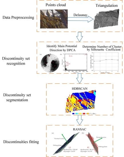
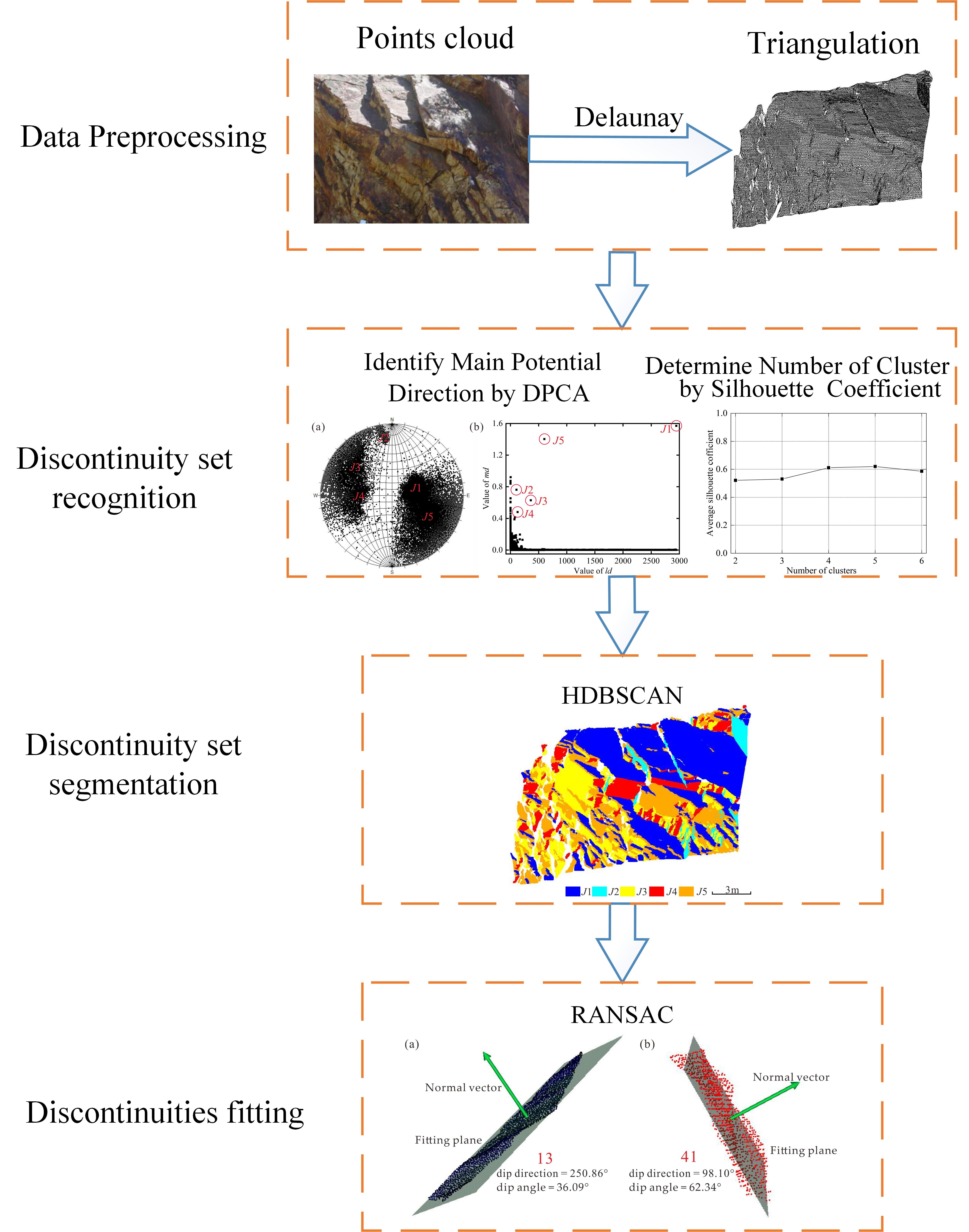
- (1)
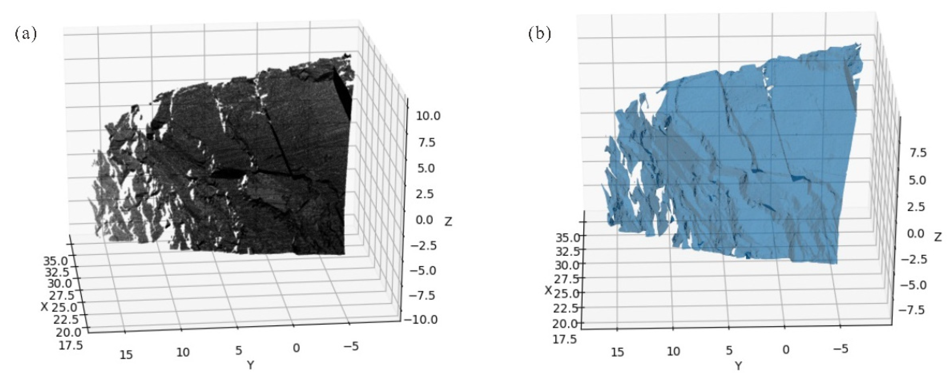
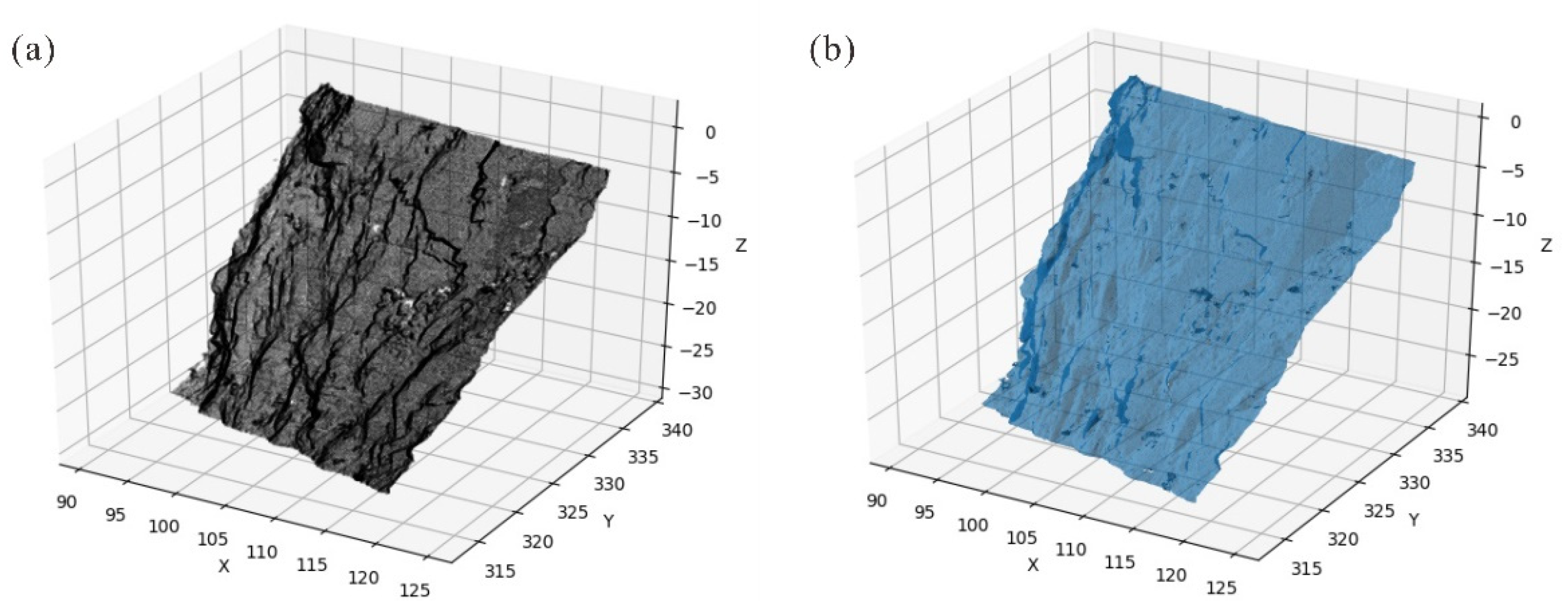
- Data preprocessing. First, remove noise points and outliers from the point clouds of the rock mass, then resample the point clouds and use the Delaunay algorithm to generate a TIN of the rock mass surface. Compared to the regular grid model, TIN has the advantages of reducing data redundancy, better performance of variation characteristics, and easy calculation [9,37].
- (2)
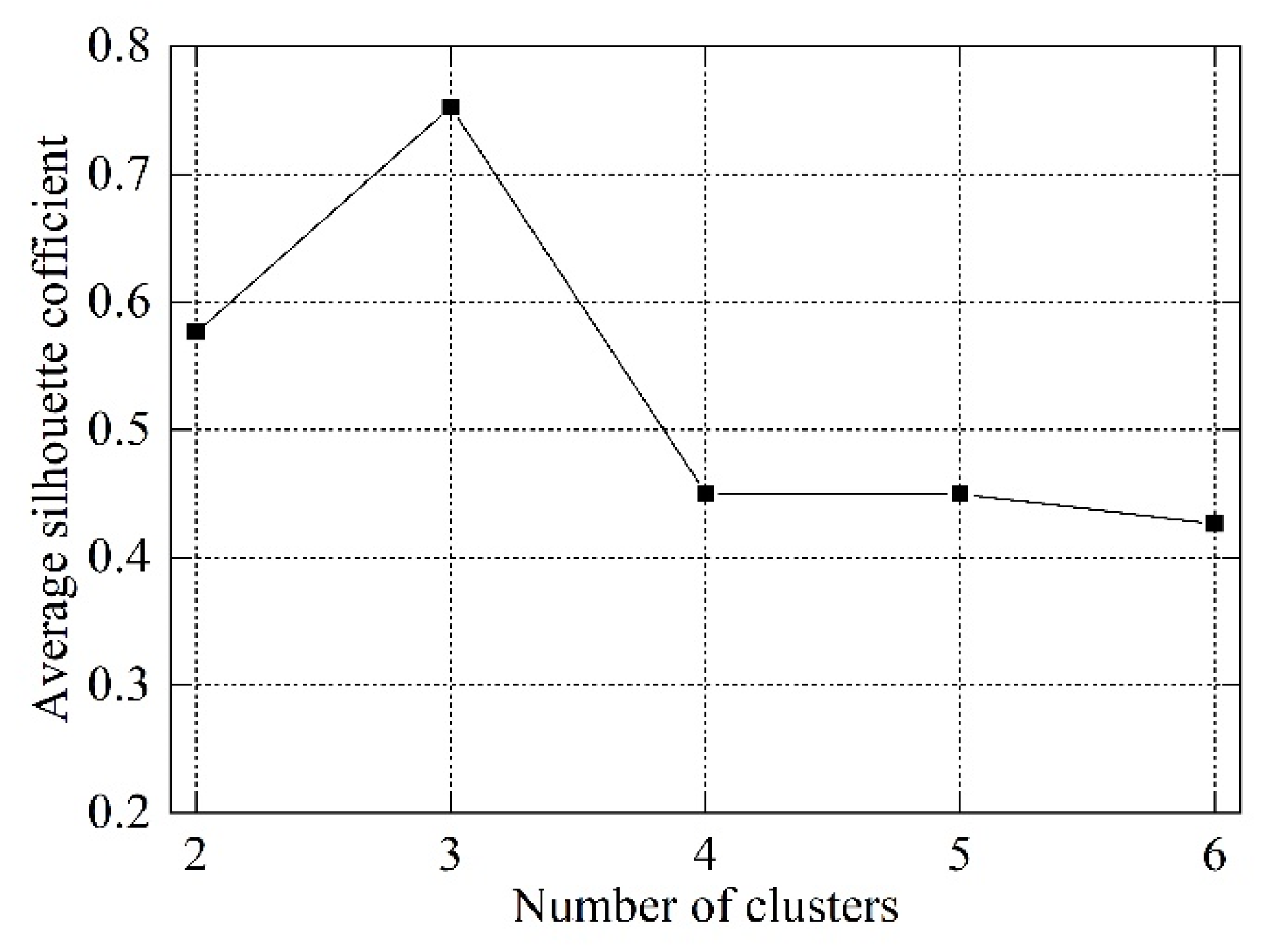
- Discontinuity set recognition. Firstly, calculate the normal vector and centroid of each triangle of the TIN. Secondly, use the DPCA to identify the main potential directions of the discontinuity set. Next, use the K-means algorithm to cluster the discontinuity set. Finally, combine the silhouette coefficient to determine the optimum clustering result. The clustering results can be expressed as Group 1, Group 2, … Group k.
- (3)
- Discontinuity set segmentation. Use the HDBSCAN algorithm to segment the discontinuity set after clustering and identify each discontinuity. Suppose each discontinuity set has m, n, …, p discontinuities, respectively.
- (4)
- Discontinuities fitting. Use the RANSAC method to fit the discontinuities and to obtain its parameters.
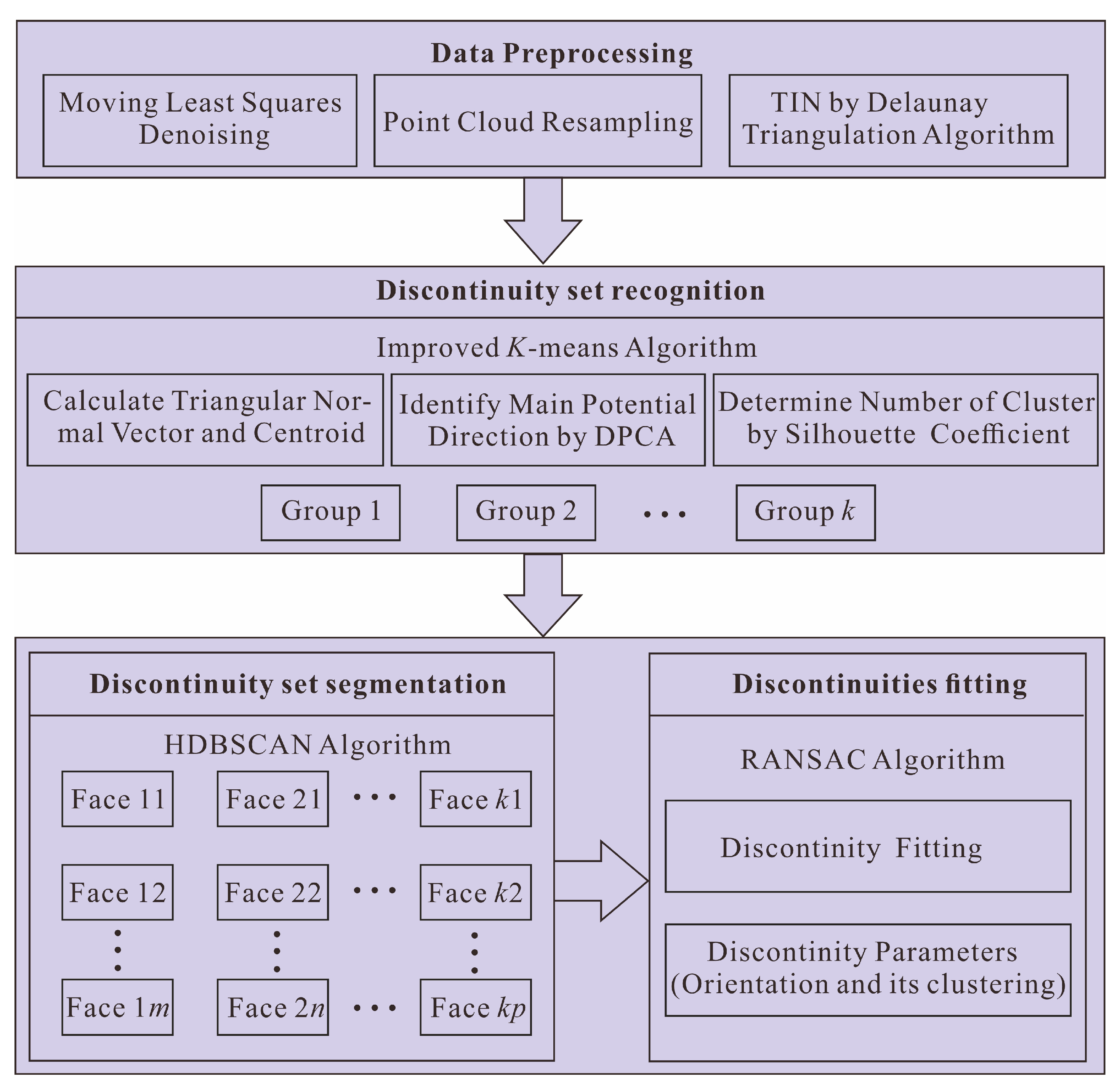
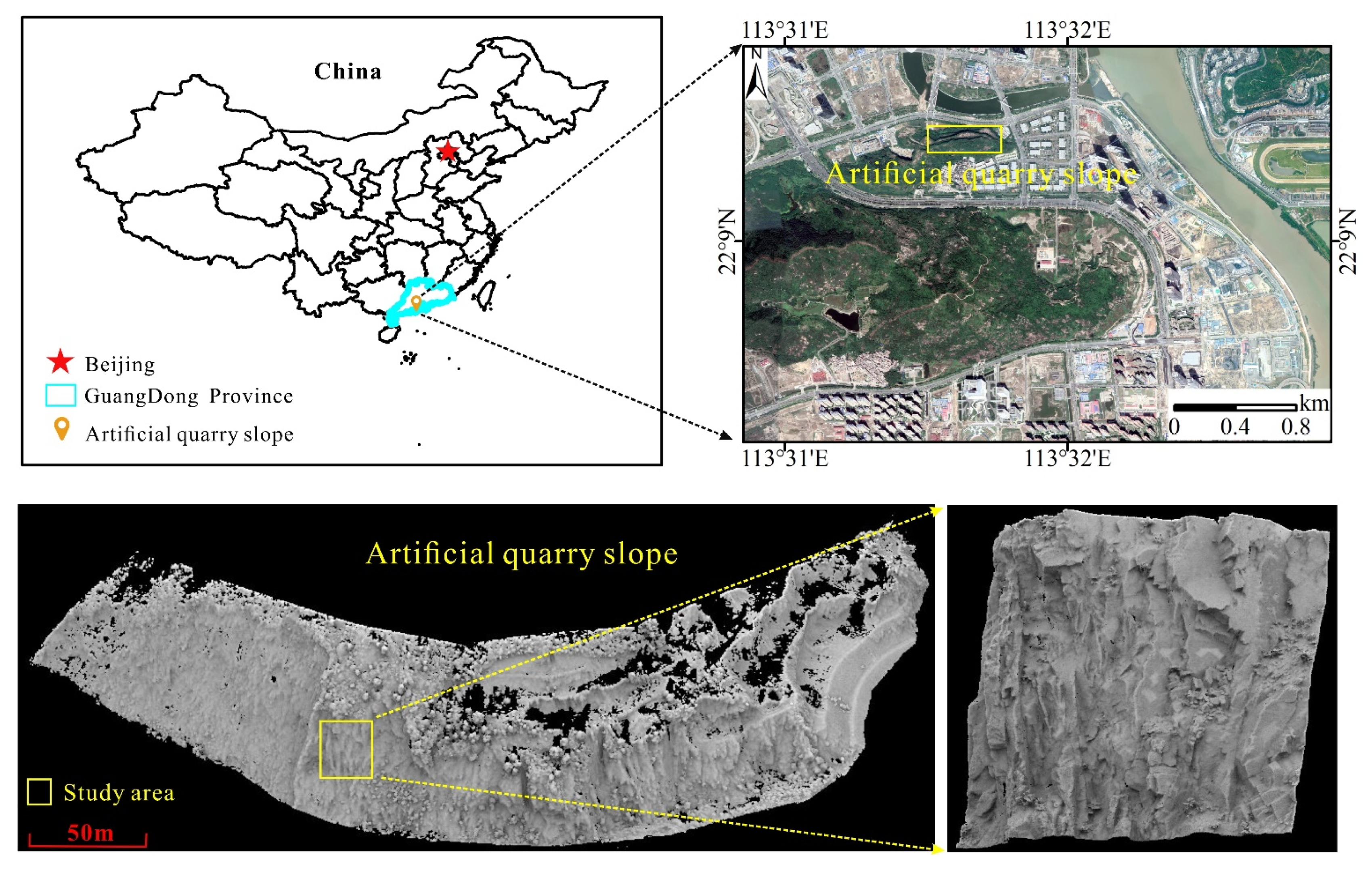
2.1. Test Data Set Description
2.2. Data Preprocessing
2.3. Discontinuity Set Recognition
2.3.1. Normal Vector and Centroid Computation
B = (Z2 − Z1)(X3 − X1) − (X2 − X1)(Z3 − Z1)
C = (X2 − X1)(Y3 − Y1) − (Y2 − Y1)(X3 − X1)
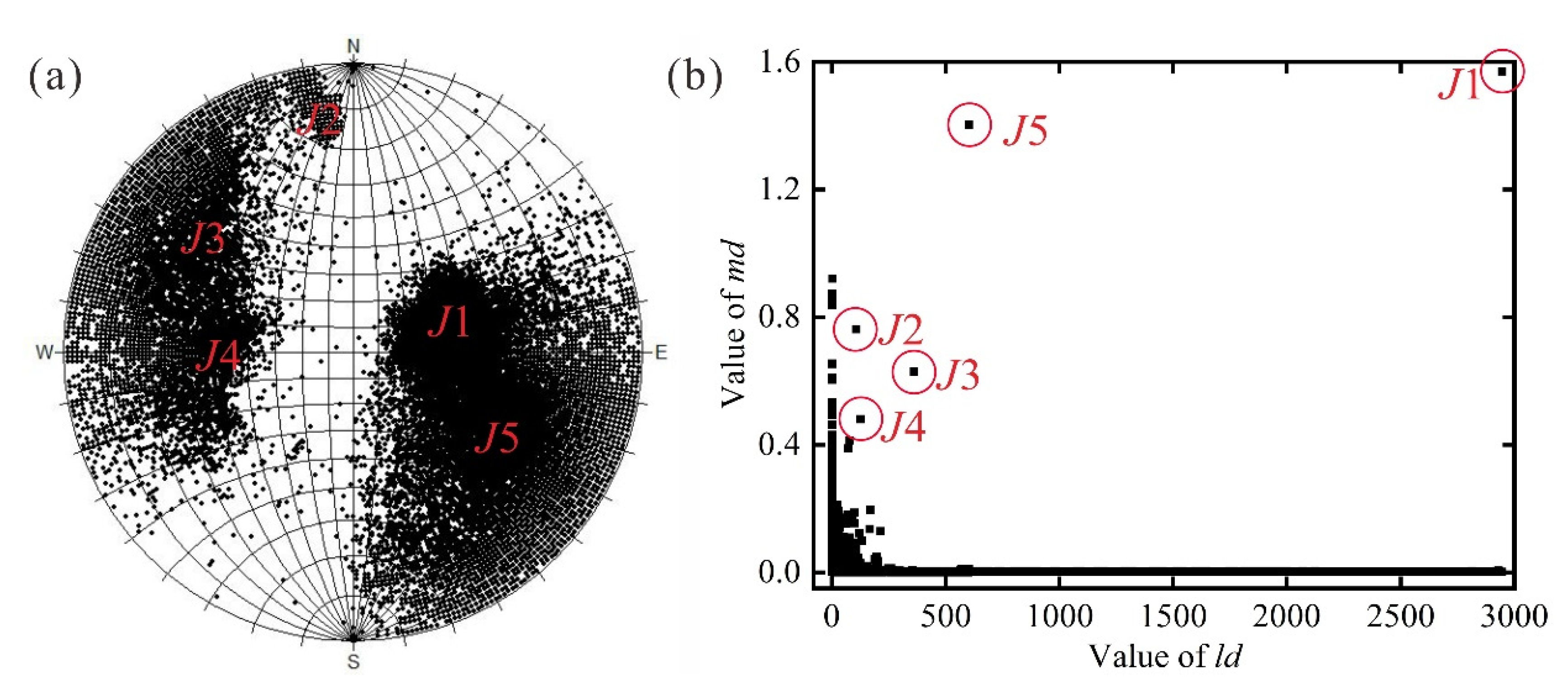
2.3.2. Determination of the Main Direction of Discontinuity Set
2.3.3. Determination of the Optimum Number of Discontinuity Set
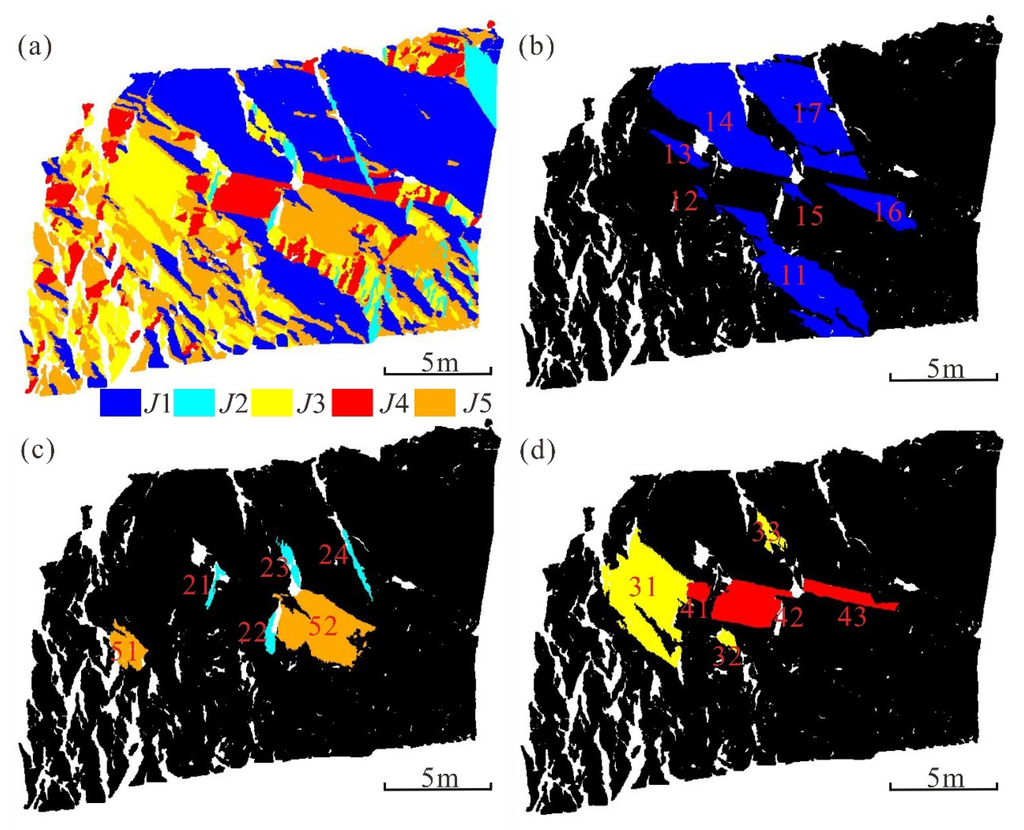
2.4. Discontinuity Set Segmentation
2.5. Discontinuities Fitting
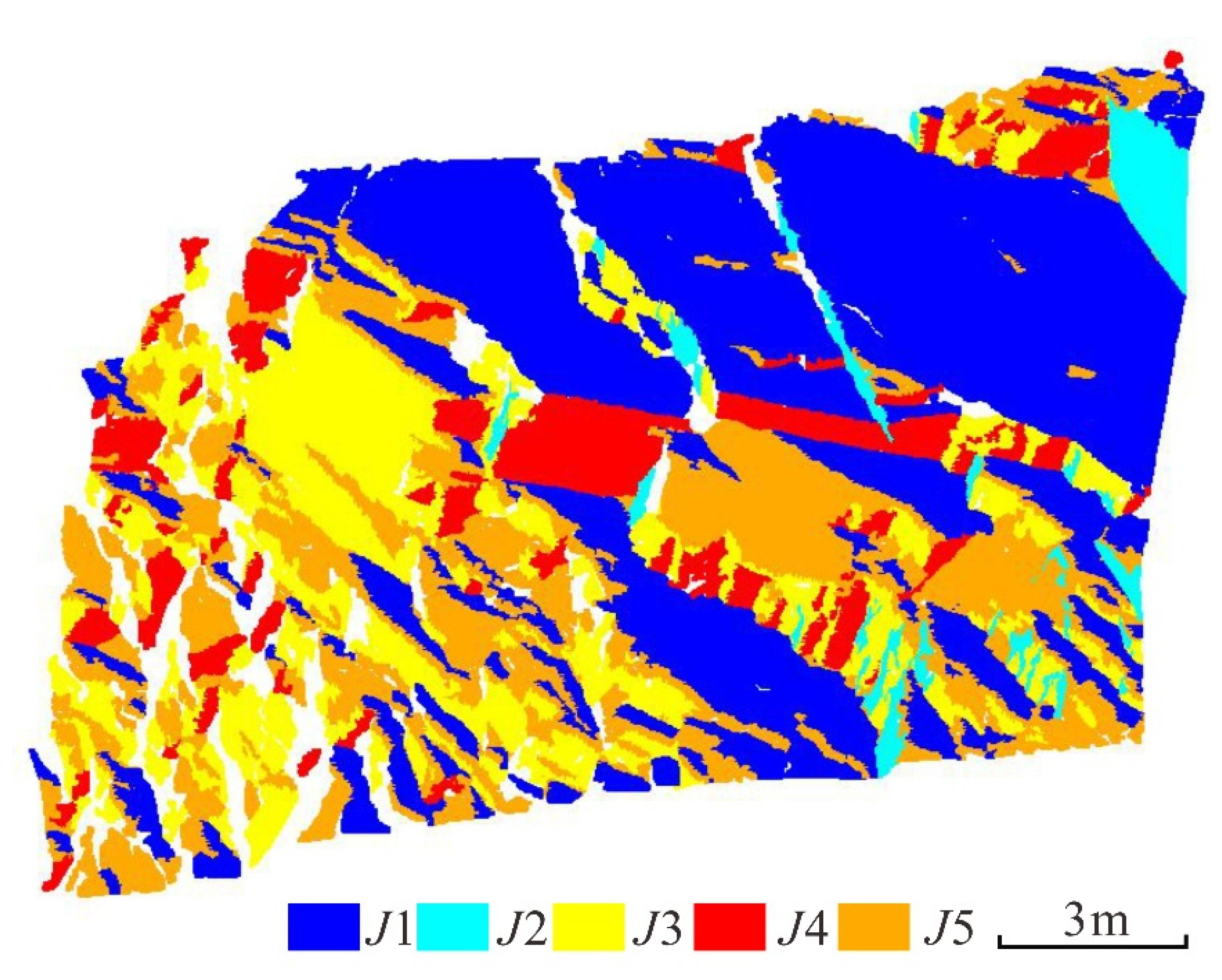
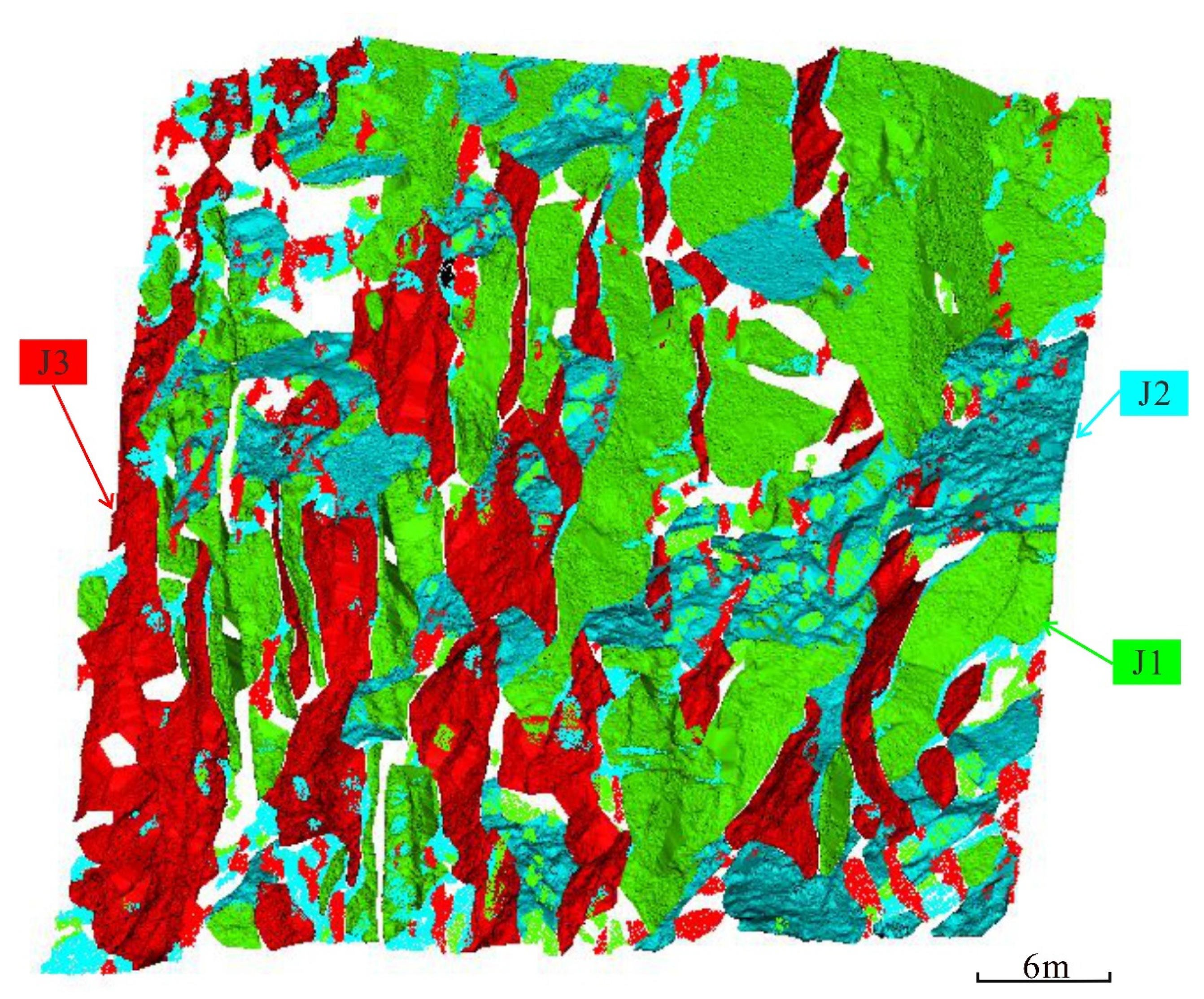
2.6. Clustering Results for the Rock Slope
3. Workflow Application to an Artificial Quarry Slope
3.1. Clustering Results of the Artificial Quarry Slope
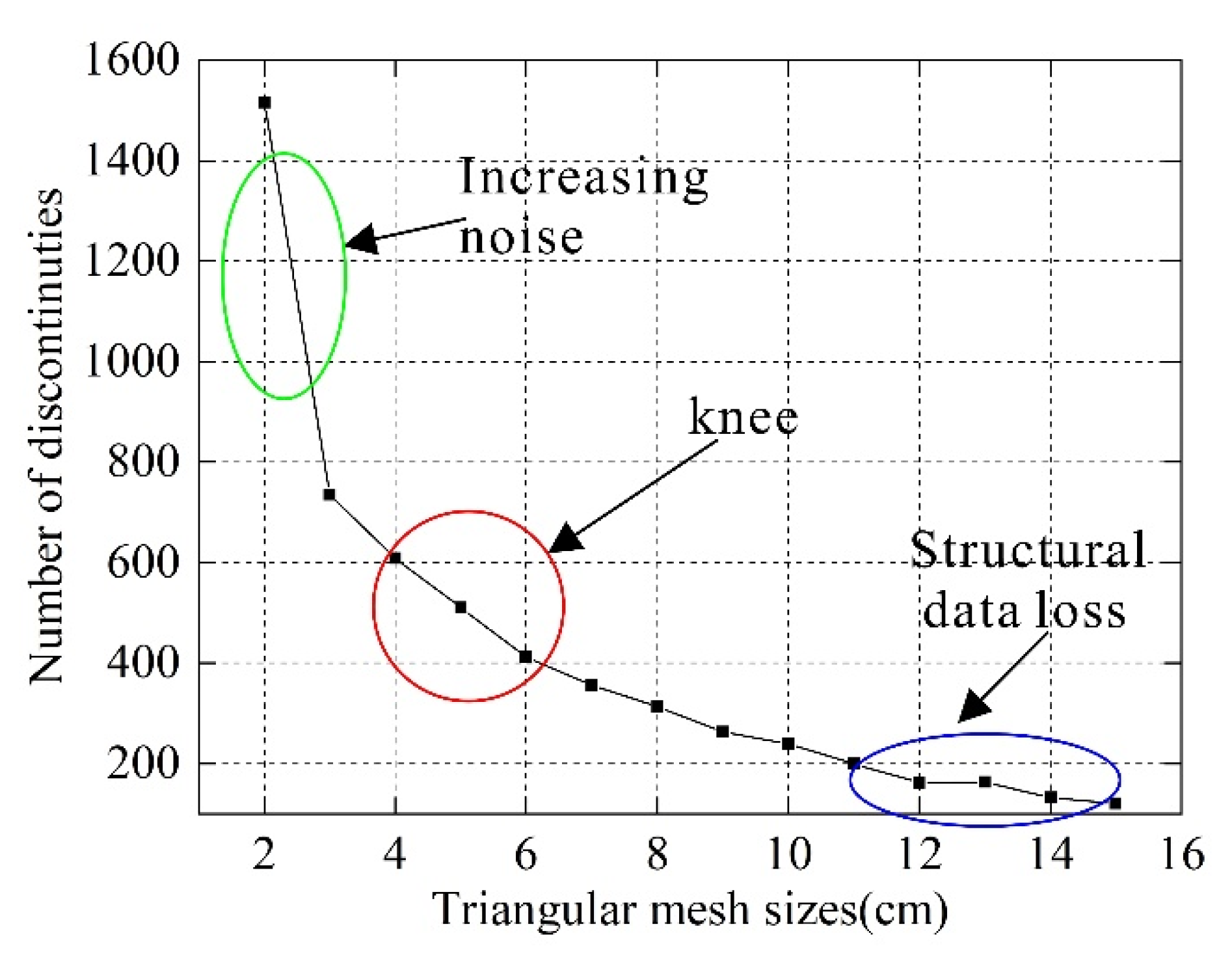
3.2. The Influence of the Triangle Mesh Size
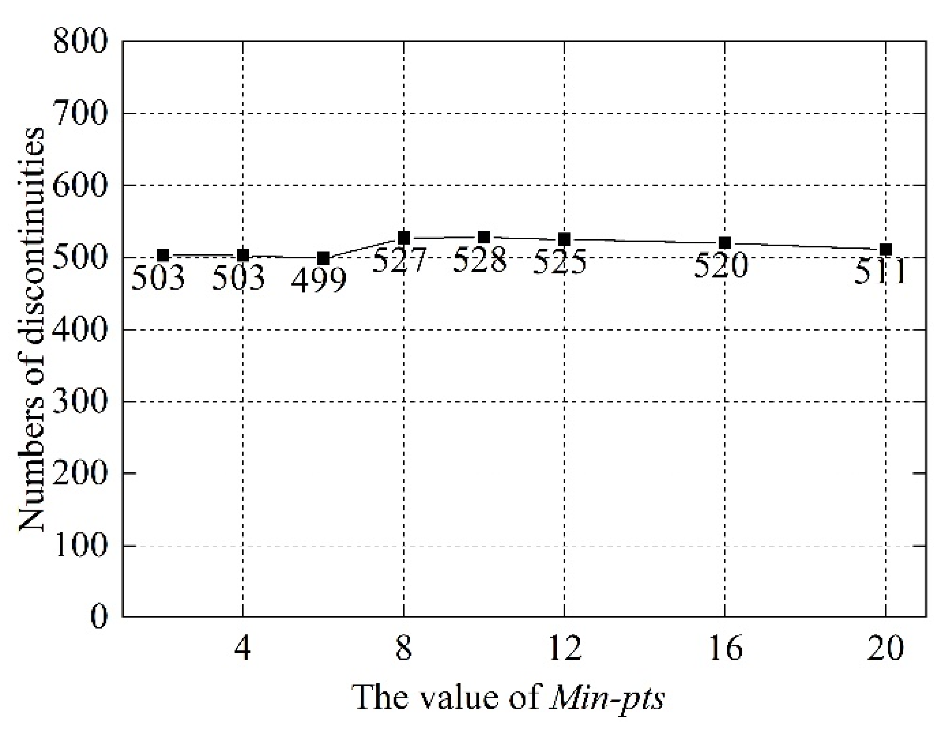
3.3. The Impact of HDBSCAN Algorithm Parameter Min-pts
4. Discussion
4.1. Comparison of the Extracting Results of the Rock Slope
4.2. Analysis of the Optimal Triangle Mesh Size
4.3. Relevant Parameters of Proposed New Method
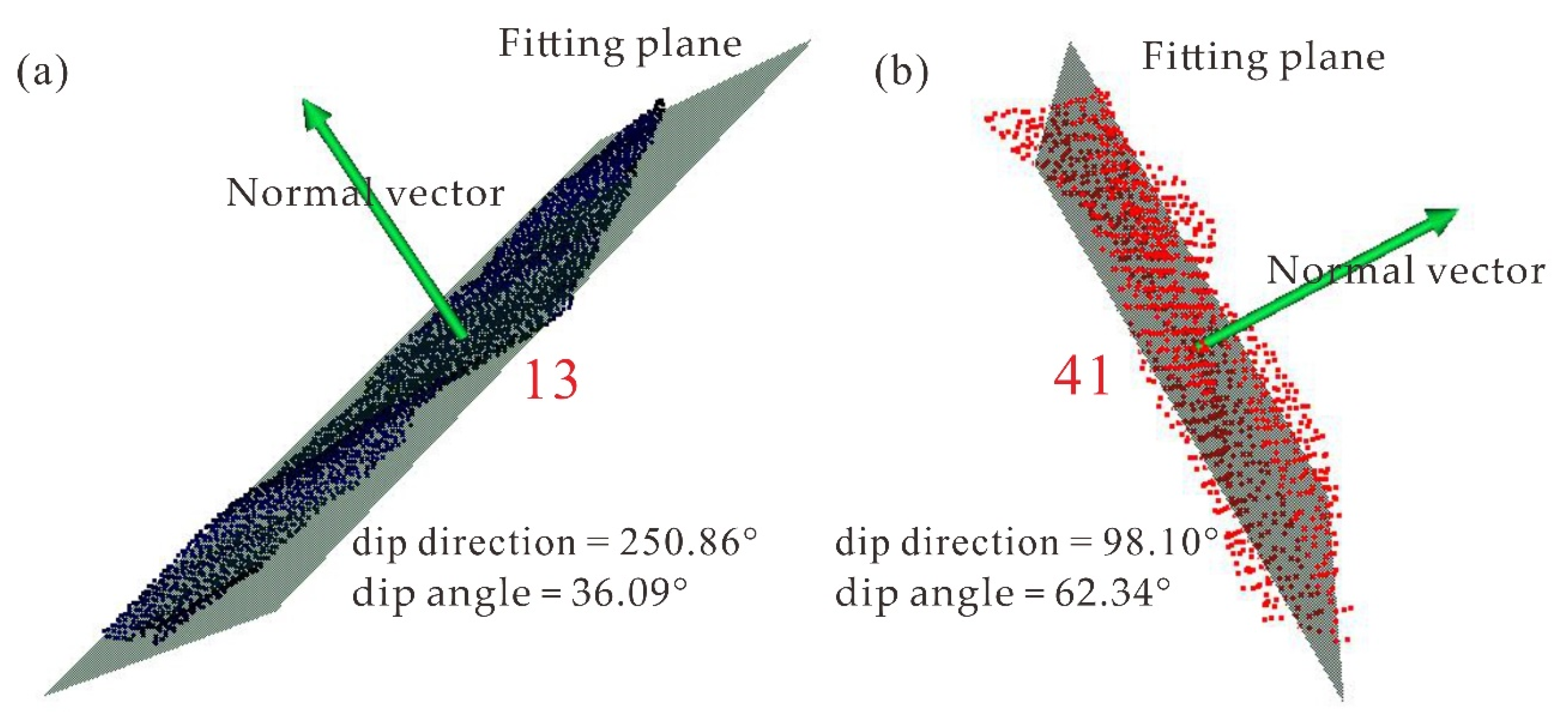
4.4. Discussion on Fitting Plane by RANSAC
4.5. Discussion on the Applicability of the New Method
5. Conclusions
Author Contributions
Funding
Institutional Review Board Statement
Informed Consent Statement
Data Availability Statement
Acknowledgments
Conflicts of Interest
References
- Guangzhong, S. On the theory of structure-controlled rockmass. J. Eng. Geol. 1993, 1, 14–18. [Google Scholar]
- Priest, S.; Hudson, J. Discontinuity spacings in rock. Int. J. Rock Mech. Min. Sci. Geomech. Abstr. 1976, 13, 135–148. [Google Scholar] [CrossRef]
- Bieniawski, Z.T. Engineering Rock Mass Classifications: A Complete Manual for Engineers and Geologists in Mining, Civil, and Petroleum Engineering; John Wiley & Sons: Hoboken, NJ, USA, 1989. [Google Scholar]
- Poropat, G.V.; Elmouttie, M.K. Automated structure mapping of rock faces. In Proceedings of the International Symposium on Stability of Rock Slopes in Open Pit Mining and Civil Engineering Situations, Brisbane, Australia, 3–6 April 2006. [Google Scholar]
- Oppikofer, T.; Jaboyedoff, M.; Blikra, L.; Derron, M.H.; Metzger, R. Characterization and monitoring of the Åknes rockslide using terrestrial laser scanning. Nat. Hazards Earth Syst. Sci. 2009, 9, 1003–1019. [Google Scholar] [CrossRef] [Green Version]
- Viero, A.; Teza, G.; Massironi, M.; Jaboyedoff, M.; Galgaro, A. Laser scanning-based recognition of rotational movements on a deep seated gravitational instability: The Cinque Torri case (North-Eastern Italian Alps). Geomorphology 2010, 122, 191–204. [Google Scholar] [CrossRef]
- Jaboyedoff, M.; Oppikofer, T.; Abellán, A.; Derron, M.H.; Loye, A.; Metzger, R.; Pedrazzini, A. Use of LIDAR in landslide investigations: A review. Nat. Hazards 2012, 61, 5–28. [Google Scholar] [CrossRef] [Green Version]
- Abellán, A.; Oppikofer, T.; Jaboyedoff, M.; Rosser, N.J.; Lim, M.; Lato, M.J. Terrestrial laser scanning of rock slope instabilities. Earth Surf. Process. Landf. 2014, 39, 80–97. [Google Scholar] [CrossRef]
- Zhang, P.; Du, K.; Zhu, H.; Zheng, W.; Tannant, D. Automated method for extracting and analysing the rock discontinuities from point clouds based on digital surface model of rock mass. Eng. Geol. 2018, 239, 109–118. [Google Scholar] [CrossRef]
- Lato, M.J.; Diederichs, M.S.; Hutchinson, D.J. Bias correction for view-limited Lidar scanning of rock outcrops for structural characterization. Rock Mech. Rock Eng. 2010, 43, 615–628. [Google Scholar] [CrossRef]
- Otoo, J.N.; Maerz, N.H.; Duan, Y.; Xiaoling, L. LiDAR and optical imaging for 3-D fracture orientations. In Proceedings of the 2011 NSF Engineering Research and Innovation Conference, Atlanta, GA, USA, 4–7 January 2011. [Google Scholar]
- Gigli, G.; Casagli, N. Semi-automatic extraction of rock mass structural data from high resolution LIDAR point clouds. Int. J. Rock Mech. Min. Sci. 2011, 48, 187–198. [Google Scholar] [CrossRef]
- Fisher, J.E.; Shakoor, A.; Watts, C.F. Comparing discontinuity orientation data collected by terrestrial LiDAR and transit compass methods. Eng. Geol. 2014, 181, 78–92. [Google Scholar] [CrossRef]
- Riquelme, A.J.; Abellán, A.; Tomás, R. Discontinuity spacing analysis in rock masses using 3D point clouds. Eng. Geol. 2015, 195, 185–195. [Google Scholar] [CrossRef] [Green Version]
- Dong, X.; Xu, Q.; Huang, R.; Liu, Q.; Kieffer, D.S. Reconstruction of Surficial Rock Blocks by Means of Rock Structure Modelling of 3D TLS Point Clouds: The 2013 Long-Chang Rockfall. Rock Mech. Rock Eng. 2019, 53, 671–689. [Google Scholar] [CrossRef] [Green Version]
- Liu, L.; Xiao, J.; Wang, Y. Major Orientation Estimation-Based Rock Surface Extraction for 3D Rock-Mass Point Clouds. Remote Sens. 2019, 11, 635. [Google Scholar] [CrossRef] [Green Version]
- Zekkos, D.; Greenwood, W.; Lynch, J.; Manousakis, J.; Athanasopoulos-Zekkos, A.; Clark, M.; Cook, K.L.; Saroglou, C. Lessons learned from the application of UAV-enabled structure-from-motion photogrammetry in geotechnical engineering. Int. J. Geoengin. Case Hist. 2018, 4, 254–274. [Google Scholar] [CrossRef]
- Kemeny, J.; Post, R. Estimating three-dimensional rock discontinuity orientation from digital images of fracture traces. Comput. Geosci. 2003, 29, 65–77. [Google Scholar] [CrossRef]
- Roncella, R.; Forlani, G. Extraction of planar patches from point clouds to retrieve dip and dip direction of rock discontinuities. In Proceedings of the Laser Scanning 2005, Enschede, The Netherlands, 12–14 September 2005. [Google Scholar]
- Potsch, M.; Schubert, W.; Gaich, A. Application of metric 3D images of rock faces for the determination of the response of rock slopes to excavation. In Proceedings of the ISRM International Symposium-EUROCK 2005, Brno, Czech Republic, 18–20 May 2005. [Google Scholar]
- Haneberg, W.C. Using close range terrestrial digital photogrammetry for 3-D rock slope modeling and discontinuity mapping in the United States. Bull. Eng. Geol. Environ. 2008, 67, 457–469. [Google Scholar] [CrossRef]
- Sturzenegger, M.; Stead, D. Quantifying discontinuity orientation and persistence on high mountain rock slopes and large landslides using terrestrial remote sensing techniques. Nat. Hazards Earth Syst. Sci. 2009, 9, 267–287. [Google Scholar] [CrossRef]
- Voge, M.; Lato, M.J.; Diederichs, M.S. Automated rockmass discontinuity mapping from 3-dimensional surface data. Eng. Geol. 2013, 164, 155–162. [Google Scholar] [CrossRef]
- Li, X.; Chen, J.; Zhu, H. A new method for automated discontinuity trace mapping on rock mass 3D surface model. Comput. Geosci. 2016, 89, 118–131. [Google Scholar] [CrossRef]
- Zhu, H.; Wu, W.; Chen, J.; Ma, G.; Liu, X.; Zhuang, X. Integration of three dimensional discontinuous deformation analysis (DDA) with binocular photogrammetry for stability analysis of tunnels in blocky rockmass. Tunn. Undergr. Space Technol. 2016, 51, 30–40. [Google Scholar] [CrossRef]
- Giordan, D.; Hayakawa, Y.; Nex, F.; Remondino, F.; Tarolli, P. Review article: The use of remotely piloted aircraft systems (RPAS) for natural hazards monitoring and management. Nat. Hazards Earth Syst. Sci. 2017, 18, 1079–1096. [Google Scholar] [CrossRef] [Green Version]
- Ester, M.; Kriegel, H.P.; Sander, J.; Xu, X. A density-based algorithm for discovering clusters in large spatial databases with noise. KDD 1996, 96, 226–231. [Google Scholar]
- Fernández, O. Obtaining a best fitting plane through 3D georeferenced data. J. Struct. Geol. 2005, 27, 855–858. [Google Scholar] [CrossRef]
- Abellán, A.; Vilaplana, J.M.; Martínez, J. Application of a long-range terrestrial laser scanner to a detailed rockfall study at Vall de Núria (Eastern Pyrenees, Spain). Eng. Geol. 2006, 88, 136–148. [Google Scholar] [CrossRef]
- Kriegel, H.; Kröger, P.; Sander, J.; Zimek, A. Density-based clustering. Wiley Interdiscip. Rev. Data Min. Know. Disc. 2011, 1, 231–240. [Google Scholar] [CrossRef]
- Jaboyedoff, M.; Metzger, R.; Oppikofer, T.; Couture, R.; Derron, M.; Locat, J.; Turmel, D. New insight techniques to analyze rock-slope relief using DEM and 3D-imaging cloud points: COLTOP-3D software. Rock Mechanics. Meeting Society’s Challenges and Demands. In Proceedings of the 1st Canada—US Rock Mechanics Symposium, Vancouver, BC, Canada, 27–31 May 2007. [Google Scholar]
- Ferrero, A.M.; Forlani, G.; Roncella, R.; Voyat, H.I. Advanced geostructural survey methods applied to rock mass characterization. Rock Mech. Rock Eng. 2009, 42, 631–665. [Google Scholar] [CrossRef]
- García-Sellés, D.; Falivene, O.; Arbués, P.; Gratacos, O.; Tavani, S.; Muñoz, J.A. Supervised identification and reconstruction of near-planar geological surfaces from terrestrial laser scanning. Comput. Geosci. 2011, 37, 1584–1594. [Google Scholar] [CrossRef]
- Wang, Y.; Feng, H.Y.; Delorme, F.É.; Engin, S. An adaptive normal estimation method for scanned point clouds with sharp features. CAD Comput. Aided Des. 2013, 45, 1333–1348. [Google Scholar] [CrossRef]
- Silverman, B.W. Density Estimation for Statistics and Data Analysis; Chapman and Hall: London, UK, 1986. [Google Scholar] [CrossRef]
- Fukunaga, K.; Hostetler, L.D. The estimation of the gradient of a density function, with application in pattern recognition. IEEE Trans. Inf. Theory 1975, 21, 32–40. [Google Scholar] [CrossRef] [Green Version]
- Chen, J.; Zhu, H.; Li, X. Automatic extraction of discontinuity orientation from rock mass surface 3D point cloud. Comput. Geosci. 2016, 95, 18–31. [Google Scholar] [CrossRef]
- Campello, R.; Moulavi, D.; Sander, J. Density-based clustering based on hierarchical density estimates. Lect. Notes Comput. Sci. 2013, 7819, 160–172. [Google Scholar] [CrossRef]
- Lato, M.; Kemeny, J.; Harrap, R.M.; Bevan, G. Rock bench: Establishing a common repository and standards for assessing rockmass characteristics using LiDAR and photogrammetry. Comput. Geosci. 2013, 50, 106–114. [Google Scholar] [CrossRef]
- Riquelme, A.J.; Abellán, A.; Tomás, R.; Jaboyedoff, M. A new approach for semi-automatic rock mass joints recognition from 3D point clouds. Comput. Geosci. 2014, 68, 38–52. [Google Scholar] [CrossRef] [Green Version]
- Alexa, M.; Behr, J.; Cohen-Or, D.; Fleishman, S.; Levin, D.; Silva, C.T. Computing and rendering point set surfaces. IEEE Trans. Vis. Comput. Graph. 2003, 9, 3–15. [Google Scholar] [CrossRef] [Green Version]
- Slob, S. Automated Rock Mass Characterisation Using 3-D Terrestrial Laser Scanning. Ph.D. Dissertation, Delft University of Technology, Delft, The Netherlands, 2010. [Google Scholar]
- Chen, J.; Xiao, S.; Wang, Q. Principles of Computer Simulation for Random Discontinuities in 3D Network; Northeast Normal University Press: Changchun, China, 1995; p. 11. [Google Scholar]
- Rodriguez, A.; Laio, A. Clustering by fast search and find of density peaks. Science 2014, 344, 1492–1496. [Google Scholar] [CrossRef] [PubMed] [Green Version]
- Gao, F.; Chen, D.; Zhou, K.; Niu, W.; Liu, H. A fast clustering method for identifying rock discontinuity sets. KSCE J. Civ. Eng. 2019, 23, 556–566. [Google Scholar] [CrossRef]
- Kulatilake, P.H.S.W.; Wu, T.H.; Wathugala, D.N. Probabilistic modelling of joint orientation. Int. J. Numer. Anal. Methods Geomech. 1990, 14, 325–350. [Google Scholar] [CrossRef]
- Priest, S.D. Discontinuity Analysis for Rock Engineering; Chapman & Hall: London, UK, 1993. [Google Scholar] [CrossRef]
- Rousseeuw, P.J. Silhouettes: A graphical aid to the interpretation and validation of cluster analysis. J. Comput. Appl. Math. 1987, 20, 53–65. [Google Scholar] [CrossRef] [Green Version]
- Tonini, M.; Abellan, A. Rockfall detection from terrestrial LiDAR point clouds: A clustering approach using R. J. Spat. Inf. Sci. 2014, 8, 95–110. [Google Scholar] [CrossRef]
- Ni, H.; Lin, X.; Zhang, J. Classification of ALS point cloud with improved point cloud segmentation and random forests. Remote Sens. 2017, 9, 288. [Google Scholar] [CrossRef] [Green Version]
- McInnes, L.; Healy, J.; Astels, S. hdbscan: Hierarchical density based clustering. J. Open Source Softw. 2017, 2, 205. [Google Scholar] [CrossRef]
- Fischler, M.A.; Bolles, R.C. Random sample consensus: A paradigm for model fitting with applications to image analysis and automated cartography. Commun. ACM 1981, 24, 381–395. [Google Scholar] [CrossRef]
- Xu, B.; Jiang, W.; Shan, J.; Zhang, J.; Li, L. Investigation on the weighted RANSAC approaches for building roof plane segmentation from LiDAR point clouds. Remote Sens. 2016, 8, 5. [Google Scholar] [CrossRef] [Green Version]
- Lato, M.; Diederichs, M.S.; Hutchinson, D.J.; Harrap, R. Optimization of LiDAR scanning and processing for automated structural evaluation of discontinuities in rockmasses. Int. J. Rock. Mech. Min. Sci. 2009, 46, 194–199. [Google Scholar] [CrossRef]


| Set | Dip Direction/Dip Angle (°) by New Method | Number of Clusters | Dip Direction/Dip Angle (°) by Riquelme et al. [40] | Number of Clusters | Δ|DD| (°) | Δ|DA| (°) |
|---|---|---|---|---|---|---|
| J1 | 248.17/34.74 | 50 | 249.04/36.66 | 59 | 0.87 | 1.92 |
| J2 | 172.27/82.22 | 14 | 172.29/83.16 | 14 | 0.02 | 0.94 |
| J3 | 134.38/81.59 | 66 | 137.33/77.87 | 56 | 2.95 | 3.72 |
| J4 | 93.67/50.82 | 45 | 092.96/48.74 | 34 | 0.71 | 2.08 |
| J5 | 286.22/65.56 | 55 | 288.45/68.22 | 57 | 2.23 | 2.66 |
| Discontinuity | Discontinuity Orientations by | Riquelme et al. in 2014 (°) | Chen et al. in 2016 (°) | New Method (°) | ||||||
|---|---|---|---|---|---|---|---|---|---|---|
| Classical Approach (°) | Riquelme et al. in 2014 (°) | Chen et al. in 2016 (°) | New Method (°) | Δ|DD| | Δ|DA| | Δ|DD| | Δ|DA| | Δ|DD| | Δ|DA| | |
| 11 | 249.18/40.23 | 246.24/39.02 | 244.62/38.38 | 246.22/38.99 | 2.94 | 1.21 | 4.56 | 1.85 | 2.96 | 1.24 |
| 12 | 264.23/57.02 | 256.86/52.3 | 256.18/52.16 | 266.09/54.72 | 7.37 | 4.72 | 8.05 | 4.86 | 1.86 | 2.30 |
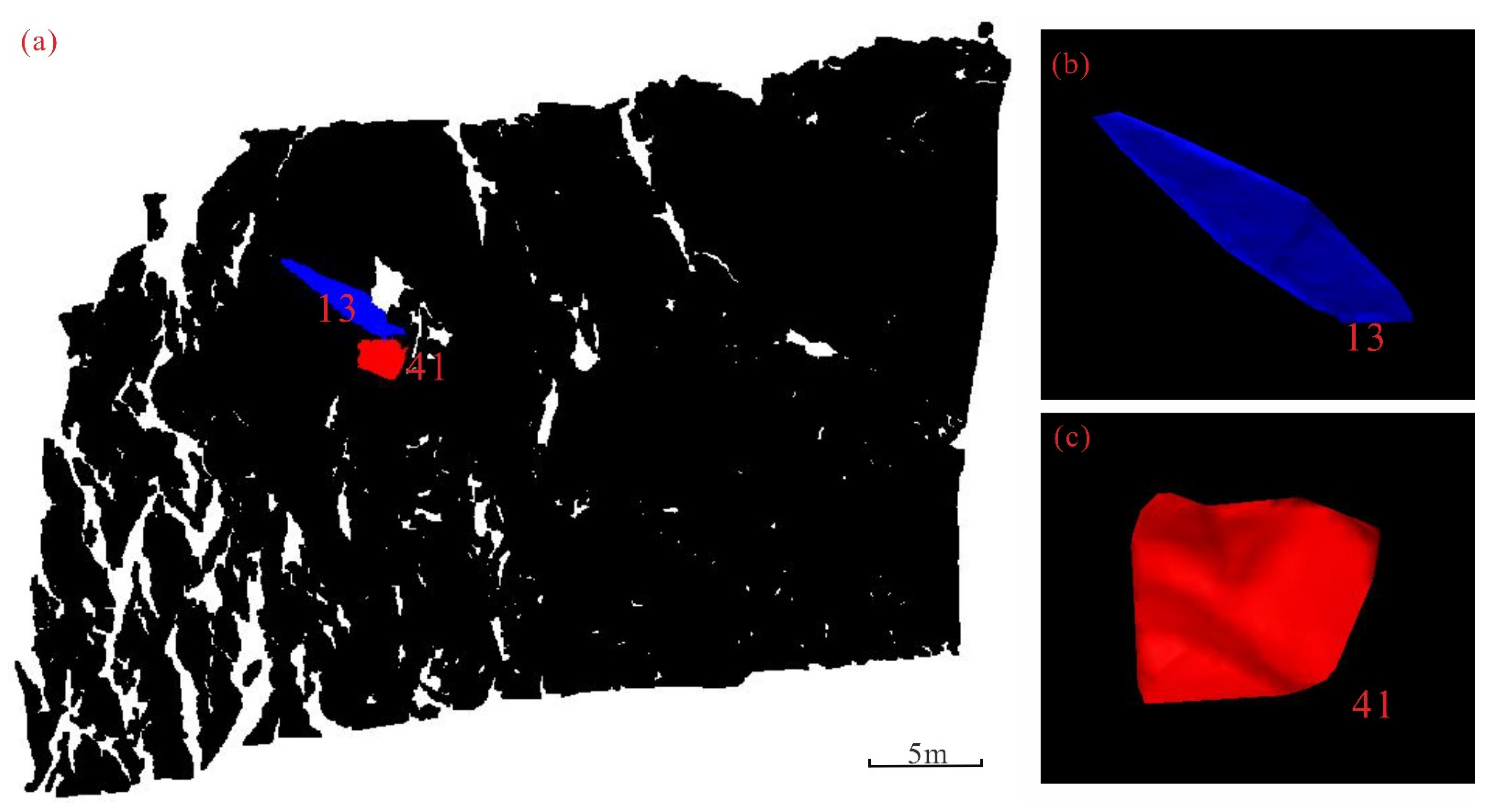
| 13 | 263.97/41.91 | 70.26/35.8 | 251.04/36.17 | 250.86/36.09 | 13.71 | 6.11 | 12.93 | 5.74 | 13.11 | 5.82 |
| 14 | 252.58/36.53 | 252.68/35.48 | 251.44/33.85 | 252.24/37.00 | 0.10 | 1.05 | 1.14 | 2.68 | 0.34 | 0.44 |
| 15 | 248.71/36.98 | 249.74/35.91 | 250.82/36.83 | 250.43/35.85 | 1.03 | 1.07 | 2.11 | 0.15 | 1.73 | 1.13 |
| 16 | 254.77/29.86 | 70.47/35.91 | 250.46/35.86 | 250.43/35.85 | 4.30 | 6.05 | 4.31 | 6.00 | 4.34 | 5.99 |
| 17 | 249.85/35.94 | 255.12/32.82 | 253.19/33.46 | 254.90/32.60 | 5.27 | 3.12 | 3.34 | 2.48 | 5.05 | 3.34 |
| 21 | 338.68/82.35 | 339.47/83.25 | 157.55/83.81 | 338.63/82.20 | 0.79 | 0.90 | 1.13 | 1.46 | 0.05 | 0.15 |
| 22 | 347.47/79.01 | 166.33/76.58 | 166.31/78.73 | 348.76/80.77 | 1.14 | 2.43 | 1.16 | 0.28 | 1.29 | 1.76 |
| 23 | 341.04/89.5 | 160.2/89.86 | 157.52/86.88 | 159.98/88.48 | 0.84 | 0.36 | 3.52 | 2.62 | 1.06 | 1.02 |
| 24 | 353.5/76.4 | 173.55/76.85 | 353.07/77.82 | 172.64/77.88 | 0.05 | 0.45 | 0.43 | 1.42 | 0.86 | 1.48 |
| 31 | 314.1/77.18 | 136.59/82.58 | 314.73/80.04 | 136.43/86.25 | 2.49 | 5.40 | 0.63 | 2.86 | 2.24 | 9.07 |
| 32 | 302.36/75.92 | 131.225/82.67 | 136.52/89.85 | 124.76/79.25 | 8.87 | 6.75 | 14.16 | 13.93 | 2.40 | 3.33 |
| 33 | 330.19/83.01 | 143.91/89.7 | 145.62/89.85 | 326.47/89.77 | 6.28 | 6.69 | 4.57 | 6.85 | 3.72 | 6.76 |
| 41 | 286.12/58.91 | 97.55/63.22 | 285.98/59.84 | 98.10/62.34 | 8.57 | 4.31 | 0.14 | 0.93 | 8.02 | 3.43 |
| 42 | 274.18/51.09 | 91.07/50.19 | 272.57/47.64 | 91.09/50.54 | 3.11 | 0.90 | 1.61 | 3.45 | 3.09 | 0.55 |
| 43 | 277.22/46.42 | 96.64/47.97 | 277.31/49.31 | 97.24/47.27 | 0.58 | 1.55 | 0.09 | 2.89 | 0.02 | 0.85 |
| 51 | 305.04/77.62 | 123.42/76.15 | 305.04/77.62 | 304.07/79.79 | 1.62 | 1.47 | 16.25 | 4.41 | 0.97 | 2.17 |
| 52 | 290.16/66.99 | 105.75/69.94 | 109.29/76.61 | 284.94/69.56 | 4.41 | 2.95 | 0.87 | 9.62 | 5.22 | 2.57 |
| Maximum deviation | 13.71 | 6.75 | 16.25 | 13.93 | 13.11 | 9.07 | ||||
| Average deviation | 3.87 | 3.03 | 4.26 | 3.92 | 3.07 | 2.81 | ||||
| Set | Dip Direction/Dip Angle (°) by New Method | Number of Clusters | Dip Direction/Dip Angle (°) by Manual Method | Number of Clusters | Δ|DD| (°) | Δ|DA| (°) |
|---|---|---|---|---|---|---|
| J1 | 163.64/61.77 | 150 | 160.22/64.58 | 60 | 3.42 | 2.81 |
| J2 | 198.56/54.61 | 188 | 189.84/44.63 | 81 | 8.72 | 9.98 |
| J3 | 225.73/66.11 | 172 | 221.93/67.76 | 64 | 3.83 | 1.65 |
| Average deviation | 5.32 | 4.81 | ||||
| Triangle Mesh Size (cm) | Number of Discontinuities | Time (h) | Precision (°) | |
|---|---|---|---|---|
| Δ|DD| | Δ|DA| | |||
| 3 | 736 | 3.25 | 4.97 | 4.53 |
| 5 | 510 | 1.39 | 5.32 | 4.81 |
| 7 | 356 | 0.36 | 6.04 | 5.73 |
| Discontinuity | Dip Direction/Dip Angle Measured by | RANSAC (°) | The Whole Points (°) | ||
|---|---|---|---|---|---|
| Classical Approach (°) | RANSAC (°) | The Whole Points (°) | Δ|DD|/Δ|DA| | Δ|DD|/Δ|DA| | |
| 13 | 263.97/41.91 | 250.86/36.09 | 248.73/34.61 | 13.11/5.82 | 15.24/7.30 |
| 41 | 286.12/58.91 | 98.10/63.34 | 96.87/64.46 | 8.02/4.43 | 9.25/5.55 |
Publisher’s Note: MDPI stays neutral with regard to jurisdictional claims in published maps and institutional affiliations. |
© 2021 by the authors. Licensee MDPI, Basel, Switzerland. This article is an open access article distributed under the terms and conditions of the Creative Commons Attribution (CC BY) license (https://creativecommons.org/licenses/by/4.0/).
Share and Cite
Wu, X.; Wang, F.; Wang, M.; Zhang, X.; Wang, Q.; Zhang, S. A New Method for Automatic Extraction and Analysis of Discontinuities Based on TIN on Rock Mass Surfaces. Remote Sens. 2021, 13, 2894. https://doi.org/10.3390/rs13152894
Wu X, Wang F, Wang M, Zhang X, Wang Q, Zhang S. A New Method for Automatic Extraction and Analysis of Discontinuities Based on TIN on Rock Mass Surfaces. Remote Sensing. 2021; 13(15):2894. https://doi.org/10.3390/rs13152894
Chicago/Turabian StyleWu, Xiang, Fengyan Wang, Mingchang Wang, Xuqing Zhang, Qing Wang, and Shuo Zhang. 2021. "A New Method for Automatic Extraction and Analysis of Discontinuities Based on TIN on Rock Mass Surfaces" Remote Sensing 13, no. 15: 2894. https://doi.org/10.3390/rs13152894