Article

In-Reservoir Waveform Retrieval for Monitoring at Groningen—Seismic Interferometry with Active and Passive Deep Borehole Data

Department of Earth Sciences, Utrecht University, Princetonlaan 8A, 3584 CB Utrecht, The Netherlands
*
Author to whom correspondence should be addressed.
Current address: Cisco Systems, Daerah Khusus Ibukota, Jakarta 12710, Indonesia.
Current address: R & D Seismology and Acoustics, Royal Netherlands Meteorological Institute (KNMI), Utrechtseweg 297, 3731 GA De Bilt, The Netherlands.
Remote Sens. 2021, 13(15), 2928; https://doi.org/10.3390/rs13152928
Submission received: 26 May 2021 / Revised: 7 July 2021 / Accepted: 20 July 2021 / Published: 26 July 2021
(This article belongs to the Special Issue Advances in Seismic Interferometry)

Abstract

:
The Groningen gas field in the Netherlands is an ideal test bed for in-situ reservoir monitoring techniques because of the availability of both active and passive in-reservoir seismic data. In this study, we use deconvolution interferometry to estimate the reflection and transmission response using active and passive borehole data within the reservoir at ∼3-km depth and separate up- and downgoing P- and S-wave fields by f-k filtering. We validate the results using synthetic data of a 1D elastic model built from sonic logs recorded in the well. The estimated full-waveform reflection response for a virtual source at the top geophone is consistent with the synthetic response. For the virtual source at the bottom geophone, the reflection response appears to be phase delayed, though its arrivals are consistent with the local subsurface geology. Similarly, the first-order estimated local transmission response successfully approximates that of the P-wave velocity in the reservoir. The study shows that reliable subsurface information can be obtained from borehole interferometry without detailed knowledge of the medium parameters. In addition, the method could be used for passive reservoir monitoring to detect velocity, attenuation, and/or interface time-lapse variations.

Graphical Abstract

1. Introduction

Seismic interferometry is a proven method to estimate the impulse response between two receivers as if one receiver acts as a virtual source and the other receiver observes the response. The main strength of this method is that it requires no knowledge of medium parameters nor of the position or timing of the actual source, as long as the wave field comes from sources within the Fresnel zones around stationary-phase locations [1].
Discovered in 1959 and started production in 1963, the Groningen gas field in the Netherlands has been one of the most prolific natural gas fields. Vast gas extraction has caused subsidence and increase in induced seismicity [2]. In 2013, a 10-sensor geophone array covering almost the entire thickness of reservoir at ∼3-km depth was placed in borehole SDM-1 for micro-seismic monitoring [3]. Aside from recording noise data, check shots at the surface were recorded to calibrate the geophone orientations. Zhou and Paulssen [4] determined the P- and S-wave velocity structure along the reservoir using noise interferometry by cross-correlation and inferred that noise is dominated by anthropogenic surface noise. A key aspect of our study is the availability of both passive (noise) and active (check-shot) borehole data, together with in-situ well-log information allowing us to very closely predict events observed on the real data.
In a more general context, this work fits in several applications and data types used in interferometry—in the sense that our approach to combining passive and active seismics with a priori knowledge extends beyond our Groningen-field borehole example. For example, Minato et al. [5] present interferometric approaches that add passive data to the more usual active crosshole experiment. In the context of earthquake-induced near-surface changes, Nakata and Snieder [6] and Nakata et al. [7] show examples of the use of passive interferometry, which could be complemented by active surface wave data. In addition, in more traditional seismology, understanding receiver functions under the language of interferometry [8] may open opportunities in the context of our work. Moreover, combing active and passive seismic data may enable or enhance interferometry-based full-waveform inversion approaches [9]. This potentially unique combination of approaches may, for instance, be of value in small-footprint monitoring of carbon sequestration [10].
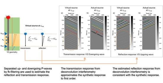
In this study, we use deconvolution interferometry to estimate the transmission and reflection response using SDM-1 borehole data, with a virtual source at the top or bottom geophone. This can be achieved by up- and downgoing wavefield separation in the f-k domain prior to deconvolution [11]. As in our case, Vasconcelos and Snieder [12] suggested that deconvolution is of most use for interferometry applications with unknown, complicated source signatures (man-made noise, natural noise). The main objective is to show that deconvolution interferometry using check shot and noise borehole data can estimate: (a) The transmission response which corresponds to the velocity structure in the reservoir, and (b) the physical reflection response within and around the reservoir. We validate the process by applying it first to the synthetic data from the 1D elastic model from well log data provided by the NAM (Nederlandse Aardolie Maatschappij).

2. Interferometric Wavefield Retrieval in a Quasi-1D Setting

2.1. Seismic Interferometry by Deconvolution

In interferometry, Green’s function or impulse response retrieval is most often done by crosscorrelation of responses at two receiver locations [1,13]. Wapenaar and Fokkema [14] mathematically derived the Green’s function representation obtained from seismic interferometry. Although it can yield an accurate representation of waves propagating between receivers, the product of cross-correlation does not only yield the impulse response. The power spectrum of the source function leaves an imprint on the estimated impulse response if not properly resolved [15]. This is often difficult if the source function is complex or unknown such as in the case of anthropogenic and natural noise. Another option for interferometry is to use deconvolution. Deconvolution interferometry yields an impulsive response without the need of an independent estimate of the source function [16] and eliminates its imprint on the impulse response. It has been used, e.g., to estimate near-surface velocities [17] and deep local imaging in borehole configuration [18], or in the context of drill-bit seismic imaging [12].
Interferometry by water-level regularized deconvolution—one of the simplest implementations of deconvolution—of two records of receivers at locations x R and x S in the frequency domain ( ω ) is expressed by:
D ^ ( x R , x S , ω ) = p ^ ( x R , ω ) p ^ * ( x S , ω ) | p ^ ( x S , ω ) | 2 + ϵ 2 < | p ^ ( x S , ω ) | 2 >
where D ^ ( x R , x S , ω ) is the response at receiver x R of a virtual source at receiver x S . As the input, p ^ ( x R , ω ) and p ^ ( x S , ω ) are the recordings at x R and x S . The asterisk denotes complex conjugation. ϵ 2 is a stabilization parameter. Here, the quantity < | p ^ ( x S , ω ) | 2 > denotes the average power over all frequencies, and ϵ 2 is a user-chosen regularization parameter: If ϵ 2 is set to too large a value, the deconvolution yields a scaled version of cross-correlation, if ϵ 2 is set to too small a value, deconvolution remains unstable.
Figure 1 illustrates the concept of 1D seismic interferometry using synthetic borehole data with an active source at the surface. All quantities in Figure 1 are in the time domain ( t ) . p ( x t o p , t ) and p ( x b o t , t ) are seismic responses observed at the geophone located at the top ( x t o p ) and bottom ( x b o t ) respectively, from the excitation of an active source at the surface (red explosion). With the top and bottom geophone at a certain distance, the first arrival observed by each geophone would have a time delay ( Δ t ) which is affected by the medium between the two geophones. In this example, the delay time of the first arrival between the two geophones is 0.074 s.
In principle, by interferometry, one can estimate the response observed at one of the geophones as if the other acts as a virtual source (blue explosion), without knowledge of the medium between the receivers. Bakulin and Calvert [19] show that the virtual source method can image structures below a complex overburden without the need for detailed overburden model building. D ( x b o t , x t o p , t ) is the estimated response observed at the bottom geophone from a virtual source at the top geophone. D ( x t o p , x b o t , t ) is the estimated response observed at the top geophone from a virtual source at the bottom geophone. In theory, the first arrival time estimated from interferometry is equal to the delay between the first arrivals of the two geophones. As for a virtual source at the bottom geophone, though it arrives at 0.074 s, the first arrival amplitude does not stand out compared to the non-physical events at an earlier time.
Events prior to the first arrivals are non-physical events. It is clear that with a virtual source at the bottom geophone, the non-physical events are stronger especially before the first arrival, indicating that the response estimation is less stable compared to a virtual source at the top geophone—we will address this in more detail in later sections. Despite the downside of the virtual source at the bottom geophone, we see that interferometry can approximate the impulse response between two receivers without the knowledge of the medium parameter between the geophones, nor the location and the timing of the actual source at the surface. Although in this example we use interferometry by deconvolution, in practice it can also be illustrated using cross-correlation.

2.2. Local Reflection and Transmission Response Estimation

To estimate the reflection responses, we follow the notation by Vasconcelos et al. [20] for regularized deconvolution. R is the reflection response for a virtual source either at the top receiver ( R t o p + ) or bottom receiver ( R b o t ): Both of these correspond to reflection responses of an infinite half-space. p + and p are the downgoing (+) and upgoing (−) waves recorded at the top or bottom geophone (subscripts t o p and b o t ). All quantities are in the frequency domain. For a virtual source at the top geophone, R t o p + can be interpreted as the estimated upgoing responses from a downgoing impulse excitation at the top geophone, recorded by other geophones (Equation (2)). The same concept applies for a virtual source at the bottom geophone. The estimated R b o t is the downgoing reflected response from an upgoing impulse excitation at the bottom geophone, recorded by the other geophones (Equation (3)). The estimated reflection response is not only locally within the reservoir, but also targeting the responses from interfaces in the medium above and below the reservoir.
p t o p = R t o p + p t o p +
p b o t + = R b o t p b o t .
Similar to the above, pseudo-transmission responses can be obtained from:
p b o t + = T t o p + p t o p +
p t o p = T b o t p b o t .
We note that, as described by [20], artifacts will be presents on the transmission wave coda under these approximate representations for transmission responses. As for local, reservoir-only transmission responses, modified versions of Equations (4) and (5) are needed to incorporate the whole wavefield.
In a more appropriate description of local transmission responses, T T E is the local (target-enclosed) transmission response with a virtual source either at the top ( T T E + ) or bottom ( T T E ). R T E is the local reflection response with a virtual source either at the top ( R T E + ) or bottom ( R T E ). This means, for example, that compared to R t o p + , R T E + only contains wave responses from the structures lying between the top and bottom receiver locations with no influence of either over- or under-burden structure. For a virtual source at the top geophone, T T E + can be interpreted as the estimated downgoing response from a downgoing impulse excitation at the top geophone, recorded by the geophones below (Equation (6)). For a virtual source at the bottom geophone, the estimated T T E is the upgoing response from an upgoing impulse excitation at the bottom geophone, recorded by the geophones above (Equation (7)):
p b o t + = T T E + p t o p + + R T E p b o t
p t o p = T T E p b o t + R T E + p t o p + .
Note that by deconvolving Equations (6) or (7) with p t o p + or p b o t , according to the chosen virtual source location, the second term at the right side of the equation is not properly accounted for, which will yield spurious-wave artifacts from the medium above and below the reservoir. Therefore, the transmission response estimation in this study is a superposition of the desired local transmission and these artifacts. Figure 2 illustrates the transmission and reflection response estimation by deconvolution interferometry. It is possible that the reflection and transmission response contains waves that reflected multiple times.
As expressed by Equations (2)–(7), the reflection and transmission estimation method requires separated up- and downgoing waves as the input for deconvolution interferometry. Without wavefield separation, full waveform interferometry can obtain reflected waves superimposed with the direct arrival (first-order transmission wave), their coda, and artifacts such as spurious arrivals [21]. Zhou and Paulssen [4] identified these events using cross-correlation interferometry. In this research, we separately estimate the reflection and transmission response by up- and downgoing wavefield separation in the f-k domain. Up-down separation prior to interferometry can suppress the artifacts of spurious arrivals from the overburden and limited acquisition aperture, thereby improving the signal-to-noise ratio [11,22].

2.3. Up- and Downgoing Wavefield Separation

Each geophone records up- and downgoing waves corresponding to their propagation direction along the array (Figure 2). The up- and downgoing P- and S-wave separation is achieved by means of f-k filtering, after Vasconcelos et al. [11]. Since the array is vertical and the medium is approximately laterally homogeneous (Figure 4), upgoing waves have negative k and downgoing waves have positive k (Figure 3). P- and S-wave separation is achieved by slope filters in the f-k domain where the slopes correspond to wave velocities, which are estimated from well-log information over the same depth interval.
Figure 3 shows the f-k spectrum from the synthetic response of an active source at the surface. It clearly shows that we can distinguish the up- and downgoing P- and S-wave based on their slope and k. Blue dashed lines represent the minimum and maximum P-wave velocity based on well-log information. The up- and downgoing wave are separated by filtering the unwanted k. The same principle of wavefield separation is applicable to the check shot and noise data. The separated up- and downgoing P-waves from f-k filtering are used as the input for deconvolution interferometry.

2.4. Setting and Overview of the Geology

The reservoir in the Groningen gas field is the Rotliegend sandstone at ∼3 km depth covered by a thin layer of basal anhydrite followed by thick Zechstein salt formation. Below the reservoir is the Carboniferous claystone formation (Figure 4). Two deep geophone arrays (SDM-1 and ZRP-1) are placed in the Loppersum area to monitor the seismicity in the reservoir. We use the borehole data from SDM-1 for which the geophone array covers almost the entire thickness of the reservoir. The array consists of 10 geophones that are aligned almost vertically.
The compressional velocities from well log data are shown in Figure 5. The two major target interfaces are the top and bottom of the Rotliegend reservoir (green and grey arrow). With a virtual source at the top or bottom geophone, we expect these interfaces to produce prominent reflection waves. Two close interfaces at the top and bottom of a thin basal anhydrite layer (blue arrows) are expected to be resolved from the true-log-derived synthetic data that have a very wide bandwidth. The wavelength is then small enough to allow us to distinguish events from each of these interfaces. As for check shot and noise data—both having considerably narrower bandwidth—events from these nearby interfaces are expected to be poorly resolved. For the transmission response estimation, the aim is to approximate the structure of the ballistic wave within the reservoir, as the coda is expected to contain artefacts as explained above. The reservoir itself contains velocity heterogeneities which would also influence the estimated reflection and transmission responses.

3. Wavefield Data Processing

The check shot and noise data of the SDM-1 borehole are recorded by 3-component geophones with a sampling rate of 2000 Hz. A total of 10 geophones with 30-m spacing are placed at 2750–3017 m depth (Figure 5). We use 4 check shot data with a 30-s record each. For noise data, we use a 24-h record (21 November 2013) divided into 2880 records of 30 s each. We use only the vertical component data, which have the strongest P wave.
We apply processing sequences as illustrated in Figure 6. Check shot and noise data are time-resampled to a 250-Hz Nyquist because the frequency content of the signal is only up to ∼80 Hz. Resampling is not applied to the synthetic data. Even though the data contain frequencies up to 80 Hz, the data are spatially aliased due to very low spatial sampling of the 10-sensor array. Aliasing is easily identified as wrap-around in f-k plot (Figure 7a). Hence, a band-pass filter of 5.5–37 Hz is applied prior to f-k filtering to suppress aliased signals and to remove very low-frequency noise (Figure 7b and Figure 8). Band-pass filtering also produces minor artifacts above the first arrival which, although insignificant, would affect further processing sequences.
Noise data are processed the same way as the check shot data assuming the source of noise only comes from above or below [4]. Indeed, f-k analysis of noise data shows that their spectrum resembles that of the check shot data with the downgoing wave dominating over the upgoing wave, except with a narrower band and weaker energy (Figure 7c). This confirms that the noise predominantly originated from above.

4. Well Log-Based Synthetic Data

To validate the process, the processing sequence of Figure 6 is first applied to the synthetic data from the 1D elastic model obtained from well log data. In the synthetic data, nine additional geophones are placed between each pair of real geophone locations to prevent aliasing and misinterpretation. A total of 91 geophones gives enough spatial sampling to clearly investigate and parameterize the process. The 1D elastic Green’s functions between sources and receivers are calculated from reflection and transmission coefficients of a layered media using real well-logs, for a plane wave with an incidence angle close to zero (near vertical). A Ricker wavelet with a peak frequency of 80 Hz is convolved with the Green’s functions to generate a synthetic response. The S-wave velocity ( V s ) is simplified to be half of the P-wave velocity ( V p ).
With the available 1D model, synthetic responses from a physical active source at the top and bottom geophone are generated. These are to be compared with the estimated response from deconvolution interferometry with a virtual source at the top and bottom geophone to validate the deconvolution process. The model also made it possible to generate only the up- or downgoing synthetic response for a physical active source at the surface to be compared with the up- and downgoing wave from f-k filtering outputs, therefore validating the wavefield separation process.

4.1. Wavefield Separation in Synthetic Data

Figure 9a shows the up- and downgoing P- and S-waves from the synthetic response and its f-k spectrum. We pass the P-wave with V p in the range 2877–6249 m/s (blue dashed lines) based on the well-log information. Figure 9b,c show the down- and upgoing P-wave and its corresponding f-k spectrum after wavefield separation in the f-k domain. The S-wave is successfully filtered out on both results. For comparison, Figure 10b,d shows up- and downgoing P waves generated directly from the model.

4.2. Reflection and Transmission Response Estimation from Synthetic Data

First, we validate the reflection and transmission response estimation by using synthetic shot data after wavefield separation. The deconvolution interferometry results are compared with the actual waves from 1D synthetic truncated model as if there is an active source at the top and bottom geophone location. For a virtual source at the top geophone, the model is truncated as if there is no medium above the virtual source. For a virtual source at the bottom geophone, the model is truncated as if there is no medium below the virtual source.
Reflection responses from interferometry and actual upgoing waves from the model are consistent for a source at the top geophone (Figure 11a,b). For a source at the bottom geophone, the estimated reflection response does match some of the actual downgoing waves (Figure 11c,d) but also displays prominent artifacts of spurious arrivals [11,21]. This is because there are insufficient upgoing waves from the bottom geophone as the V p log to create the synthetic response is only available up to ∼50 m below the bottom geophone; thus there are not enough reflection interfaces to generate substantial upgoing waves. If deconvolution is applied on the same truncated model as in Figure 11b,d, the deconvolution result and the actual wave are consistent. Despite having prominent artifacts, the reflection response estimation with a virtual source at the bottom geophone (Figure 11c) successfully resolves the strong anhydrite reflection interface at ∼2143 m depth (yellow arrow in Figure 5).
The transmission response from interferometry displays an explicit match with the actual up- or downgoing wave from the model only to the first-order transmission (Figure 12). Some of the transmission responses at a later time only subtly match with the actual wave from the model (colored dashed lines). This dissimilarity is due to artifacts in the right side of Equations (6) and (7) that is not eliminated by deconvolution. The artifacts in this application of seismic interferometry is described in Section 8. As in the reflection response estimation, if deconvolution is applied on the same truncated model as in Figure 12b,d, the transmission response and the actual wave are consistent.
Although containing artifacts of spurious arrivals, plus insufficient input of the upgoing waves because of depth limitation of the V p log data, deconvolution interferometry using synthetic shot data successfully estimates the actual reflection and transmission events. Reflection and transmission response estimation using a homogenous medium above the top geophone eliminates the artifacts at the wave coda. This heuristic argument supports the existence of spurious events in deconvolution interferometry.

5. Wavefield Separation in Active and Passive Field Data

The same f-k filtering parameters as in the synthetic shot data are applied to the check shot and noise data. For check shot and noise data, the band-pass filter of 5.5–37 Hz is applied prior f-k filtering to suppress aliasing. The data are first resampled to 250 Hz Nyquist as in the processing sequence of Figure 6.
Figure 13 and Figure 14 show the up- and downgoing wavefield separation process in the f-k domain using check shot and noise data. As in the synthetic data, f-k filtering in the check shot data is unable to fully resolve events at the boundary of the seismic section. The change of slope at the section boundary in Figure 13a appears linear in Figure 13b (red dashed line). The f-k filter also introduces artifacts before the first-arrival downgoing wave. These shortcomings of the f-k filtering process are expected to affect the deconvolution interferometry result.

6. Reflection and Transmission Response Estimation from Field Data

For check shot and noise data, final transmission and reflection response estimates result from the time integration of the deconvolution using every 30-s time interval records. A total of four check shots records and 2884 noise interval records are used for time integration. Although the check shots are not exactly located above the well, the waves recorded at the geophone array are within the stationary phase region as described in Section 7.

6.1. Active Field Data

The deconvolution interferometry results for check shot data are compared with the actual up- and downgoing waves from the model in Figure 15 and Figure 16. Colored dashed lines represent events in the interferometry result that match the actual up- or downgoing waves. Red-dashed lines indicate the first arrival times based on the well-log V p data. For interpretation convenience, non-physical events above this first arrivals are muted in the reflection response. The corresponding number for some of the lines represents the interpretation of the nth-order transmitted/reflected wave as it reflected multiple times from the two major reflection interfaces at the top and bottom of the reservoir. The actual up- and downgoing wavefields are generated from the same truncated 1D elastic model as in Figure 11b and Figure 12b for a virtual source at the top geophone, and as in Figure 11d and Figure 12d for a virtual source at the bottom geophone. To make a relevant comparison with a low-frequency signal of check shot and noise data, the up- and downgoing synthetic responses are now generated using a wavelet with a peak frequency of 18 Hz.
The ballistic-arrival transmission response (Figure 15a and Figure 16a) agrees well with the first arrival travel time based on the V p log (red-dashed line). This suggests that deconvolution interferometry can estimate wave responses that in turn yield a smooth velocity structure within the reservoir.
Figure 15c shows the reflection response, which can be interpreted as the reflected direct arrival (red-dashed line) as it meets reflection interface within and around the reservoir. The intersection of the known direct wave arrival times with the reflection events on the gathers provides an estimate of reflection depth. A strong reflection is visible shortly after the first arrival reaches the bottom geophone, indicating that there is a reflection interface not far beneath the bottom geophone. From the V p log, we identify this as a physical reflection from the interface at ∼3033 m (grey arrow in Figure 5), which is the contact interface of the Rotliegend reservoir and the Upper Carboniferous. The estimated transmission and reflection response using a virtual source at the top geophone also indicates what we interpreted as the 1st to 4th order wave that has reflected multiple times from two major interfaces at the top and bottom of the Rotliegend reservoir (Figure 15a,c).
Unlike Figure 11c, now by using real data, a strong reflection is visible in Figure 16c around the top geophone, suggesting a reflector around the top geophone. We identify this as a physical reflection from a thin layer of basal anhydrite at ∼2721–2765 m (blue arrow in Figure 5). With a dominant frequency of 18 Hz and average velocity of 5900 m/s, the general threshold for a vertical resolution of 82 m (a quarter of dominant wavelength) is well above the thickness of this layer (∼44 m), hence the data cannot resolve both interfaces. Hence, the strong reflection around the top geophone in Figure 16c is a superposition of the top and bottom reflections of the basal anhydrite. The estimated transmission and reflection response using a virtual source at the bottom geophone also indicates what we interpreted as the 1st to 4th order wave that has reflected multiple times from two major interfaces at the top and bottom of the reservoir (Figure 16a,c).
Both reflection responses from a virtual source at the top and bottom geophone (Figure 15c and Figure 16c) also indicate a clear reflection at ∼2940 m (orange arrow) due to reservoir heterogeneity, although these reflections appear to be phase delayed when comparing field- and synthetics-based wavefields. One cause for the phase delay observed at this bandwidth may be the interference of short-period, higher-order multiples that seem to be present at these arrival times, as seen in e.g., Figure 11d. A better understanding the cause of this phase delay is the subject of ongoing investigation.
Compared with the up- and downgoing wavefields from synthetic data (Figure 15b,d and Figure 16b,d), the estimated reflection responses give a good agreement for a virtual source at the top geophone, but not for a virtual source at the bottom geophone as it appears to be phase delayed. This suggests that deconvolution interferometry using check shot data can extract the physical reflection response from actual reflection interfaces accurately by using the top geophone as a virtual source. As is the case for synthetic data, the estimated first-order transmission response using check shot data can approximate the response of the P-wave velocity structure in the reservoir. Despite having spurious-arrival artifacts in its coda, we can subtly follow several of the 1st to higher-order transmitted/reflected wave events that interact with the two major reflection interfaces at the top and bottom of the reservoir. Note that because the f-k filter cannot resolve slopes at the boundaries of the field seismic sections (namely, at the very top and bottom), the corresponding interferometry results at the section boundaries are prone to artefacts unlike in our synthetics, because there we can simply model the wavefields beyond the length of the actual array to ensure accuracy in f-k filtering.

6.2. Passive Field Data

The same principle and processing parameters we used for the check shot data are also applied using the noise data to estimate the transmission and reflection response with a virtual source at the top and bottom geophones (Figure 17). The estimated transmission responses in Figure 17a,c approximate the first arrivals travel time based on the V p log (red-dashed line). Figure 17b,d show that estimated reflection response from noise data is consistent with the check shot data. The interpreted 1st to 4th order waves from the noise data are also consistent with the interpretation of the check shot data, although the transmission/reflection events in the noise data lack continuity and have smaller amplitude, for instance, the 3rd order wave in Figure 17a. This could be due to a more unstable spectral distribution in the f-k domain and a lower dominant frequency (16 Hz) compared to the check shot data, which directly affects the wavefield separation and deconvolution process. The green-dashed line in Figure 17d resembles the strong anhydrite reflection in Figure 16d, however, it could also be a spurious arrival as the amplitude is not as strong.
The consistency of the results indicates that deconvolution interferometry using noise borehole data can also retrieve the physical reflections and velocity structure in the reservoir. We believe the transmission estimates to be sufficiently accurate with regard to the direct arrivals, but its coda is a superposition of actual transmitted arrivals and artifacts [20]. Thus, these non-physical events must be properly accounted for and one must be extra cautious in interpreting the estimated transmission and reflection response. This requires multidimensional deconvolution using data from both top and bottom receivers at once, and is beyond the scope of this study.
We have seen that interferometry using active and passive borehole data enables us to obtain reliable subsurface information without knowledge of the velocity model between the source and geophones, where sometimes conventional methods fail to image the data below complex media such as a sub-salt flank [12,19]. The interferometry application in this research is using the P-wave from vertical component records only. The same concept is also applicable to the S-wave from the horizontal component of the check shot or noise records. Zhou and Paulssen [4], for instance, approximated the S-wave velocity in the reservoir and determined azimuthal anisotropy from the S-wave polarizations. High sensitivity to small medium changes in passive borehole interferometry and its high degree of repeatability is useful for reservoir monitoring [4,15,23,24]. Thus, one can detect the velocity and/or interface variations in the reservoir for time-lapse studies with lower cost and less effort compared to conventional approaches [25]. With identifiable time-lapse changes in the reservoir, it can also be used to monitor induced seismicity, which in the Groningen reservoir is caused by gas production [2].

7. Check-Shot Stationary Phase Analysis

One pre-requisite for seismic interferometry to yield physically meaningful arrivals is that the wave must come from sources within Fresnel zones around stationary points [1]. Stationarity is expected for our deep borehole data because even though the check shots are at some distance away from the well at the surface (Figure 18a), multiples and scattered waves within the medium between the surface and the geophone array are sufficient to produce almost vertically propagating wavepaths relative to the array (Figure 18b).
Stationary phase analysis is performed by deconvolution interferometry at varying time windows and duration using SP2 (Figure 18c) which is the furthest check shot from the well at the surface. Figure 19 and Figure 20 show the results of every 0.8-s time window, with a 0.6-s overlap starting from the 4.7-s record. The first arrival travel time in SP2 is at ∼5.24 s, thus the first time window already includes a small part of the signal. Records prior to the first arrivals consist of noise data only.
The transmission responses from time-varying interferometry are exceptionally consistent, thus stationary, no matter which time window and duration we chose from the 30-s record, as long as we include the signal any time after the first arrivals at 5.24 s. The reflection wave is only consistent if we input the early time window when it includes the strong first arrival and its first strong reflected wave which has the more stable f-k spectrum and frequency content. At much later time windows (>5.7 s), f-k and spectrogram analysis display more unstable spectral distributions. This directly affects the wavefield separation and deconvolution processes. Consistent deconvolution results around the first arrival time window suggests that the wave that arrives at the geophone array is within the stationary phase region.

8. Spurious Arrivals in Seismic Interferometry

Although sources within the Fresnel zone are sufficient to retrieve the arrivals characterized by those stationary contributions, ideally isotropic illumination is required for seismic interferometry. Isotropic illumination in a borehole configuration means that the energy of the up- and down-propagating fields is equal, thus that the net power flux in the up- and downgoing wave is close to zero [1]. In our data where the sources originate at the surface, stronger downgoing waves compared to the upgoing waves (Figure 7) indicates predominantly one-sided illumination. This causes an incomplete cancellation of the contribution from different stationary points which could lead to a bias in the Green’s function retrieval such as the occurrence of spurious arrival artifacts [1,21], as we have seen in the interferometry results in the synthetic and field data. In one-sided illumination, energy radiated by the interferometric virtual source differs from that radiated by placing a real physical source at the receiver location, which radiates energy in all directions [12,15]. This is partially what causes the difference in the estimated response from interferometry and the actual response from a physical active source in the synthetic data (Figure 11 and Figure 12).
For the estimated reflection responses, minor artifacts at the coda are more of the consequences of stabilization parameter ( ϵ 2 ) in the water-level regularized deconvolution to mitigate notches in the spectrum of p ^ ( x S , ω ) in Equation (1). Artifacts produced by up-down separation in the f-k domain (Figure 13) and frequency filtering process (Figure 8) can also contribute to artifact generation in interferometry. For the estimated transmission response, we have seen at the right side of Equations (6) and (7) that what we estimate is not only the local, reservoir-only transmission response, but also artifacts resulted from waves that are propagating from the medium below the bottom geophone for a virtual source at the top, and from the medium above the top geophone for a virtual source at the bottom. Hence, the product of the transmission response estimation in this study is a superposition of the local transmission response and the artifacts due to spurious waves from the medium outside the spatial coverage of the geophone array. This is one of the reasons for the low signal-to-noise ratio in the estimated local transmission responses in Figure 12. In the reflection response estimation, this type of artifact is not incorporated in the equation because we do not only estimate the local, reservoir-only reflection responses, but also the reflection from the medium outside the spatial coverage of the array (e.g., anhydrite reflection at ∼2143-m depth, Rotliegend–Carboniferous interface below the bottom geophone). Thus, Equations (2) and (3) are valid for reflection response estimation. If we are targeting only the local reflection within the reservoir, Equations (2) and (3) must also be modified as in Equations (6) and (7) to incorporate spurious artifacts from the medium below the bottom geophone for a virtual source at the top, and from the medium above the top geophone for a virtual source at the bottom.
To minimize interferometric artefacts, Bakulin and Calvert [19] suggested a solution by applying a time window that aims to select the strong direct waves only as the input. This is the case for Figure 19 and Figure 20, which are using an input time window within strong first arrivals only. As a result, Figure 21 shows that it suppresses high-frequency events which could be the frequency content of spurious arrivals artefact (arrow at ∼32 Hz). In this study, spurious arrivals from the overburden are suppressed by the up- and downgoing wavefield separation prior to interferometry [11,16,22]. However, we have seen that minor spurious arrivals still occur partially due to one-sided illumination characteristic in the field data. Furthermore, it is very prominent in the synthetic data for reasons described in Section 4.2 and in the previous paragraph.
Mehta et al. [22], Snieder et al. [21], and Vasconcelos et al. [11] suggested that these spurious artifacts can be suppressed if sources below the target reflectors are included, thus aiming for isotropic illumination. In deconvolution interferometry, excessive multiple scattering can also potentially extract a response that is closer to the full elastic response [12]. Such a condition can be met if the geophone array is deep enough, the overburden is highly heterogeneous, and for a long recording time. However, it is difficult to predetermine the period of time required for recording time that would allow for sufficient multiple scattering to compensate the lack of sources [12]. When applicable, a more advanced technique to suppress these artifacts is by multi-dimensional deconvolution which not only corrects for irregular source distribution and spurious arrivals due to one-sided illumination, it also improves control over the radiation behavior of the virtual source and accounts for dissipation [15]. Finally, we also point out that spurious arrivals in interferometry, though not corresponding to physical events of an otherwise actual-source at the virtual source location, are the by-product of interference of physical waves present in the recorded data. As such, when handled properly, interferometry-generated spurious arrivals can be used to extract information about the medium. For example, Draganov et al. [10,26] explore using such spurious arrivals for the estimation of attenuation, and for time-lapse monitoring, such as in CO 2 sequestration.

9. Conclusions

Given the availability of well-logs, together with active and passive borehole data, the Groningen field is an ideal test bed for interferometry-based monitoring techniques. Here, our interferometry application to estimate the in-reservoir reflection and transmission response requires up- and downgoing P- and S-wave separation as the input. Wavefield separation is performed in the f-k domain and the process is validated using the synthetic responses from the 1D elastic model. Using active and passive deep borehole data, we estimate the full-waveform reflection responses by deconvolution interferometry for a virtual source at the top geophone which is consistent with the actual responses from the synthetic data as if we have an active source at the top geophone. As for virtual source at the bottom geophone, the reflection response appears to be phase delayed, though it contains arrivals consistent with the geology. We show that the estimated reflection wave is physically meaningful, resulting from actual subsurface reflection interfaces. Using the same principle, a first-order estimated transmission wave yields a direct wave in which the slope corresponds to the P-wave velocity in the reservoir. However, it is important that in interpreting coda waves from interferometry, non-physical events such as spurious arrival artifacts must be accounted for, or least be considered during interpretation, especially when the source distribution is not isotropic, i.e., when illumination is directionally uneven. In the more extreme cases, one-sided illumination can lead to bias in impulse response retrieval. Spurious arrivals could, however, be further explored for monitoring, as shown by other studies. Interferometry with time-varying input windows shows that the results remain consistent, providing a reliable indication that the waves contributing to the interferometry result are within the stationary phase region. This interferometry application is applicable in similar borehole settings as long as the waves are within a stationary phase region, which is one of the requirements in seismic interferometry. Reliable subsurface information obtained from active and passive borehole interferometry in the Groningen gas field can be of use for reservoir monitoring by detecting velocity and/or interface time-lapse variations, subsurface imaging without requiring the velocity model of the overburden medium nor the medium within the reservoir, and further understanding of the mechanics of seismicity induced by gas extraction with a substantially reduced cost and effort compared to conventional approaches. We stress that it is the combination of well-log information, active and passive borehole data in Groningen that allows one to validate and understand interferometric response in detail—so that their reliability is verified for passive monitoring purposes.

Author Contributions

Conceptualization, I.V. and H.P.; investigation, M.F.A.; data curation, W.Z.; methodology, I.V.; software, M.F.A., W.Z. and I.V.; writing—original draft preparation, M.F.A.; writing—review and editing, I.V.; visualization, M.F.A.; supervision, I.V. and H.P. All authors have read and agreed to the published version of the manuscript.

Funding

M.F.A. thanks the Indonesia Endowment Fund for Education, abbreviated as LPDP, from the Indonesian Ministry of Finance for sponsoring his MSc study.

Institutional Review Board Statement

Not applicable.

Informed Consent Statement

Not applicable.

Data Availability Statement

The data that were used in this study are available from EPOS-NL, https://epos-nl.nl/ (accessed on 20 May 2021).

Acknowledgments

We thank Kees Wapenaar (TU Delft) for providing the 1D elastic modeling code used to generate our synthetic data. We are very grateful to the NAM for kindly providing the velocity models, borehole, and well-log data. M.F.A. conducted this research as part of completing his MSc in Earth Sciences at Utrecht University.

Conflicts of Interest

The authors declare no conflict of interest.

References

  1. Wapenaar, K.; Draganov, D.; Snieder, R.; Campman, X.; Verdel, A. Tutorial on seismic interferometry: Part 1—Basic principles and applications. Geophysics 2010, 75, 75A195–75A209. [Google Scholar] [CrossRef] [Green Version]
  2. Van Thienen-Visser, K.; Breunese, J. Induced seismicity of the Groningen gas field: History and recent developments. Lead. Edge 2015, 34, 664–671. [Google Scholar] [CrossRef] [Green Version]
  3. NAM. Study and Data Acquisition Plan Induced Seismicity in Groningen—Winningsplan 2016; NAM Report; NAM: Kota Administrasi Jakarta Pusat, Indonesia, 2016. [Google Scholar]
  4. Zhou, W.; Paulssen, H. P and S velocity structure in the Groningen gas reservoir from noise interferometry. Geophys. Res. Lett. 2017, 44, 785–791. [Google Scholar] [CrossRef]
  5. Minato, S.; Matsuoka, T.; Tsuji, T.; Draganov, D.; Hunziker, J.; Wapenaar, K. Seismic interferometry using multidimensional deconvolution and crosscorrelation for crosswell seismic reflection data without borehole sources. Geophysics 2011, 76, SA19–SA34. [Google Scholar] [CrossRef] [Green Version]
  6. Nakata, N.; Snieder, R. Near-surface weakening in Japan after the 2011 Tohoku-Oki earthquake. Geophys. Res. Lett. 2011, 38. [Google Scholar] [CrossRef] [Green Version]
  7. Nakata, N.; Snieder, R.; Tsuji, T.; Larner, K.; Matsuoka, T. Shear wave imaging from traffic noise using seismic interferometry by cross-coherence. Geophysics 2011, 76, SA97–SA106. [Google Scholar] [CrossRef] [Green Version]
  8. Galetti, E.; Curtis, A. Generalised receiver functions and seismic interferometry. Tectonophysics 2012, 532-535, 1–26. [Google Scholar] [CrossRef]
  9. Sager, K.; Ermert, L.; Boehm, C.; Fichtner, A. Towards full waveform ambient noise inversion. Geophys. J. Int. 2017, 212, 566–590. [Google Scholar] [CrossRef]
  10. Draganov, D.; Heller, K.; Ghose, R. Monitoring CO2 storage using ghost reflections retrieved from seismic interferometry. Int. J. Greenh. Gas Control 2012, 11, S35–S46. [Google Scholar] [CrossRef]
  11. Vasconcelos, I.; Snieder, R.; Hornby, B. Imaging internal multiples from subsalt VSP data—Examples of target-oriented interferometry. Geophysics 2008, 73, S157–S168. [Google Scholar] [CrossRef] [Green Version]
  12. Vasconcelos, I.; Snieder, R. Interferometry by deconvolution: Part 2—Theory for elastic waves and application to drill-bit seismic imaging. Geophysics 2008, 73, S129–S141. [Google Scholar] [CrossRef]
  13. Curtis, A.; Gerstoft, P.; Sato, H.; Snieder, R.; Wapenaar, K. Seismic interferometry—Turning noise into signal. Lead. Edge 2006, 25, 1082–1092. [Google Scholar] [CrossRef]
  14. Wapenaar, K.; Fokkema, J. Green’s function representations for seismic interferometry. Geophysics 2006, 71, SI33–SI46. [Google Scholar] [CrossRef]
  15. Wapenaar, K.; Slob, E.; Snieder, R.; Curtis, A. Tutorial on seismic interferometry: Part 2—Underlying theory and new advances. Geophysics 2010, 75, 75A211–75A227. [Google Scholar] [CrossRef] [Green Version]
  16. Vasconcelos, I.; Snieder, R. Interferometry by deconvolution: Part 1—Theory for acoustic waves and numerical examples. Geophysics 2008, 73, S115–S128. [Google Scholar] [CrossRef]
  17. Mehta, K.; Snieder, R.; Graizer, V. Extraction of near-surface properties for a lossy layered medium using the propagator matrix. Geophys. J. Int. 2007, 169, 271–280. [Google Scholar] [CrossRef] [Green Version]
  18. Liu, Y.; Arntsen, B.; Wapenaar, K.; van der Neut, J. Combining inter-source seismic interferometry and source-receiver interferometry for deep local imaging. In SEG Technical Program Expanded Abstracts 2014; Society of Exploration Geophysicists: Tulsa, OK, USA, 2014; pp. 5107–5112. [Google Scholar]
  19. Bakulin, A.; Calvert, R. The virtual source method: Theory and case study. Geophysics 2006, 71, SI139–SI150. [Google Scholar] [CrossRef]
  20. Vasconcelos, I.; Ravasi, M.; Kritski, A.; van der Neut, J.; Cui, T. Local, reservoir-only reflection and transmission responses by target-enclosing extended imaging. In SEG Technical Program Expanded Abstracts 2017; Society of Exploration Geophysicists: Tulsa, OK, USA, 2017; pp. 5289–5293. [Google Scholar]
  21. Snieder, R.; Wapenaar, K.; Larner, K. Spurious multiples in seismic interferometry of primaries. Geophysics 2006, 71, SI111–SI124. [Google Scholar] [CrossRef] [Green Version]
  22. Mehta, K.; Bakulin, A.; Sheiman, J.; Calvert, R.; Snieder, R. Improving the virtual source method by wavefield separation. Geophysics 2007, 72, V79–V86. [Google Scholar] [CrossRef] [Green Version]
  23. Behm, M. Feasibility of borehole ambient noise interferometry for permanent reservoir monitoring. Geophys. Prospect. 2017, 65, 563–580. [Google Scholar] [CrossRef]
  24. Bakulin, A.; Mateeva, A.; Mehta, K.; Jorgensen, P.; Ferrandis, J.; Herhold, I.S.; Lopez, J. Virtual source applications to imaging and reservoir monitoring. Lead. Edge 2007, 26, 732–740. [Google Scholar] [CrossRef]
  25. Zhou, W.; Paulssen, H. Compaction of the Groningen gas reservoir investigated with train noise. Geophys. J. Int. 2020, 223, 1327–1337. [Google Scholar] [CrossRef]
  26. Draganov, D.; Ghose, R.; Ruigrok, E.; Thorbecke, J.; Wapenaar, K. Seismic interferometry, intrinsic losses and Q-estimation. Geophys. Prospect. 2010, 58, 361–373. [Google Scholar] [CrossRef]
Figure 1. Illustration of 1D seismic interferometry with a synthetic active source at the surface. Black arrow depicts a wave path from the corresponding source. x is the geophone location at the top and bottom (subscripts top and bot). (1) Response observed by geophone at x t o p from excitation at the surface. (2) Response observed by geophone at x b o t from excitation at the surface. (3) Estimated response observed at x b o t as if we have a virtual source at x t o p . (4) Estimated response observed at x t o p as if there is a virtual source at x b o t .
Remotesensing 13 02928 g001
Figure 2. Illustration of the reflection and transmission response by deconvolution interferometry with an active source at the surface (red explosion) and virtual source at the top and bottom geophone (blue explosions). The solid and dashed lines indicate the down- and upgoing waves. Orange and light blue lines portray wave paths that are recorded at x t o p and x b o t (both up- and downgoing wave).
Remotesensing 13 02928 g002
Figure 3. Up- and downgoing wavefield separation in the f-k domain using synthetic data. The area between the blue dashed line represents the P-wave energy that we pass. The slope of the dashed line is based on the chosen V p limit.
Remotesensing 13 02928 g003
Figure 4. Overview of the geology in the SDM-1 well proximity [4]; provided by the Nederlandse Aardolie Maatschappij (NAM). The target of micro-seismic monitoring is the Rotliegend gas reservoir, lying under the basal anhydrite layer and above the Carboniferous formation.
Remotesensing 13 02928 g004
Figure 5. SDM-1 compressional velocities ( V p ). Left: Overall V p log. Right: Local V p log around the depth interval of interest.
Remotesensing 13 02928 g005
Figure 6. Processing flowchart of transmission and reflection response estimation using interferometry with a virtual source at the top (output 1) and bottom geophone (output 2).
Remotesensing 13 02928 g006
Figure 7. F-k analysis of check shot and noise data. (a) F-k plot shows wrap-around indicating aliased signal. (b) Frequency content of check shot data before and after the band-pass filter to suppress aliasing. (c) F-k plot of noise data. Its spectral distribution resembles the check shot data.
Remotesensing 13 02928 g007
Figure 8. Check shot data before and after the band-pass filter. Although reducing aliasing, it introduces minor artifact above the first arrivals.
Remotesensing 13 02928 g008
Figure 9. Wavefield separation of synthetic shot data in the f-k domain with a physical source at the surface. (a) The up- and downgoing wave and its f-k spectrum. (b) Downgoing wave and its f-k spectrum. (c) Upgoing wave and its f-k spectrum.
Remotesensing 13 02928 g009
Figure 10. F-k filter outputs compared with the up- and downgoing wave generated by the model. (a,b) show the downgoing wave from the f-k filter and the model. (c,d) show the upgoing wave from the f-k filter and the model.
Remotesensing 13 02928 g010
Figure 11. Reflection response estimation using synthetic shot data. (a,c) show the reflection response with a virtual source at the top and bottom geophone. (b) The upgoing wave from an actual source at the top geophone. (d) Downgoing wave from an actual source at the bottom geophone. Colored dashed lines represent events in the interferometry result that match with the up- or downgoing events from the model. The dashed circle shows artifacts of spurious arrivals.
Remotesensing 13 02928 g011
Figure 12. Transmission response estimation using synthetic shot data. (a,c) show the transmission response with a virtual source at the top and bottom geophone. (b) The downgoing wave from an actual source at the top geophone. (d) Upgoing wave from an actual source at the bottom geophone. Colored dashed lines represent events in the interferometry result that match with the up- or downgoing events from the model. Dashed circle shows artifacts of spurious arrivals.
Remotesensing 13 02928 g012
Figure 13. Wavefield separation of check shot data in the f-k domain. (a) The up- and downgoing wavefield and its f-k spectrum. (b) The downgoing wavefield and its f-k spectrum. Red-dashed circle shows poorly resolved events at the seismic section boundary. (c) The upgoing wavefield and its f-k spectrum. Red-dashed circle shows the area that contains artifacts of the f-k filter above the first-order downgoing wave.
Remotesensing 13 02928 g013
Figure 14. Wavefield separation of noise data in the f-k domain. (a) The up- and downgoing wavefield and its f-k spectrum. (b) The downgoing wavefield and its f-k spectrum. (c) The upgoing wavefield and its f-k spectrum.
Remotesensing 13 02928 g014
Figure 15. Interferometry using check shot data for a virtual source at the top geophone. (a,b) show the estimated transmission response and the actual downgoing wave from the model. (c,d) show the estimated reflection response and the actual upgoing wave from the model. The up- and downgoing wavefield synthetic response is generated from the same truncated model as in Figure 11b and Figure 12b, except now using an 18-Hz peak frequency wavelet.
Remotesensing 13 02928 g015
Figure 16. Interferometry using check shot data for a virtual source at the bottom geophone. (a,b) show the estimated transmission response and the actual upgoing wave from the model. (c,d) show the estimated reflection response and the actual downgoing wave from the model. The up- and downgoing wave synthetic response is generated from the same truncated model as in Figure 11d and Figure 12d, except now using an 18-Hz peak frequency wavelet.
Remotesensing 13 02928 g016
Figure 17. Interferometry using noise data. (a,b) show the estimated transmission and reflection response for a virtual source at the top geophone. (c,d) are the estimated transmission and reflection response for a virtual source at the bottom geophone.
Remotesensing 13 02928 g017
Figure 18. Four check shot locations around the SDM-1 well. (a) Map view of check shot locations. SP2 is the furthest check shot from the well (black arrow). (b) The cross-section of the map view at the Y-coordinate of the well location. Ray path with more scattering (red-dashed line) arrives at the geophone array with a smaller incident angle than the direct ray path from the source (yellow-dashed line). (c) SP2 check shot raw record that is used for time-varying interferometry. Only the 4.7–6.1-s record is shown from the full 30-s record.
Remotesensing 13 02928 g018
Figure 19. Transmission response from time-varying interferometry of check shot SP2. Times above each panel indicate the time window of the check shot record used as an input for interferometry.
Remotesensing 13 02928 g019
Figure 20. Reflection response from time-varying interferometry of check shot SP2. Times above each panel indicate the time window of the check shot record used as an input for interferometry.
Remotesensing 13 02928 g020
Figure 21. Frequency content of reflection responses with and without time windowing from a virtual source at the top geophone using check shot data. (a) Frequency content of Figure 15c, which is using a full time window of 30 s. (b) Frequency content of Figure 20c, which is using a time window selecting only the strong arrivals at 5.1–5.9 s. The arrow points to what could be the frequency content of the artifact.
Remotesensing 13 02928 g021
Publisher’s Note: MDPI stays neutral with regard to jurisdictional claims in published maps and institutional affiliations.

