An Adaptive Surface Interpolation Filter Using Cloth Simulation and Relief Amplitude for Airborne Laser Scanning Data

Abstract

Separating point clouds into ground and nonground points is an essential step in the processing of airborne laser scanning (ALS) data for various applications. Interpolation-based filtering algorithms have been commonly used for filtering ALS point cloud data. However, most conventional interpolation-based algorithms have exhibited a drawback in terms of retaining abrupt terrain characteristics, resulting in poor algorithmic precision in these regions. To overcome this drawback, this paper proposes an improved adaptive surface interpolation filter with a multilevel hierarchy by using a cloth simulation and relief amplitude. This method uses three hierarchy levels of provisional digital elevation model (DEM) raster surfaces with thin plate spline (TPS) interpolation to separate ground points from unclassified points based on adaptive residual thresholds. A cloth simulation algorithm is adopted to generate sufficient effective initial ground seeds for constructing topographic surfaces with high quality. Residual thresholds are adaptively constructed by the relief amplitude of the examined area to capture complex landscape characteristics during the classification process. Fifteen samples from the International Society for Photogrammetry and Remote Sensing (ISPRS) commission are used to assess the performance of the proposed algorithm. The experimental results indicate that the proposed method can produce satisfying results in both flat areas and steep areas. In a comparison with other approaches, this method demonstrates its superior performance in terms of filtering results with the lowest omission error rate; in particular, the proposed approach retains discontinuous terrain features with steep slopes and terraces.

1. Introduction

Airborne laser scanning (ALS) technology, which employs airborne light detection and ranging (LiDAR) systems, is quickly becoming the mainstream method for rapidly and reliably capturing accurate earth surface information over large-scale areas [1,2]. It has been widely applied in various fields, such as digital elevation model (DEM) generation [1,3,4,5], urban building model reconstruction [6,7,8], and forest resource management [9,10,11]. As the laser pulses of ALS technology are able to penetrate through vegetation to the terrain surface [12], ALS is suitable for acquiring high-precision terrain. However, raw ALS data usually contain numerous surface objects (such as buildings, vegetation and vehicles) and outliers caused by multipath reflection. Therefore, the separation of the ground (or nonground) points from the raw data is the critical process in the generation of high-resolution DEMs; this process is referred to as ground filtering for ALS point clouds [2].

In recent decades, many ground filtering methods have been proposed to separate ground points from point clouds. According to the filtering strategies used, these methods can be grouped into five primary categories: interpolation-based [13,14,15,16,17,18,19,20,21,22,23,24,25,26], slope-based [27,28,29,30,31,32,33], morphological-based [34,35,36,37,38,39,40], segmentation-based [41,42,43,44,45,46,47,48,49], and simulation-based [50,51,52,53] approaches. Each category has shown its advantages in dealing with different kinds of topography. Among these categories, interpolation-based methods are regarded as very robust for separating ground and nonground points in forested environments and have been used in the majority of situations [54].

An interpolation-based filtering method starts by selecting ground seeds and then iteratively interpolates the ground surface with densified ground points to progressively approximate the terrain surface. The ground points are separated from the remaining surface measurement points by measuring their proximity to the interpolated ground surface, which is typically the residual threshold of elevation. These filtering methods usually adopt thin plate spline (TPS) interpolation and perform well in flat areas [23]. However, they have faced challenges in terms of the terrain accuracy of interpolated surfaces and the measure of proximality. The former is constrained by the selected seeds, while the latter is determined by the constructed residual threshold.

These TPS interpolation-based methods built upon the local minimum point algorithm use a moving window to select initial ground seeds, and the window size is usually set according to the maximum building size of a given area [13,14,20,21]. The setting of the window size constrains the choice of seeds to a small number of points, which may lead to the generation of a poor initial ground surface. Furthermore, most TPS interpolation-based filters adopt a fixed residual threshold for all points to distinguish ground and nonground points at each hierarchical level [21,22,23]. This fixed residual threshold is obviously not adapted to complex terrain, especially in a steep region where the residual threshold is larger than that in a flat region. To improve the abovementioned filtering methods for such complex terrains, the concept of topographic slope is utilized to construct the residual thresholds, as different terrain points may present different slopes [13,14]. However, the slope parameter is unable to accurately capture discontinuous terrain features with steep slopes and terraces.

The selection of seeds and the residual thresholds construction method restrict the filtering performance of the previously described TPS interpolation-based methods. This paper proposes an improved adaptive surface interpolation (ASI) method with a multilevel hierarchy by using a cloth simulation to improve the selection of seeds and the relief amplitude to adaptively set residual thresholds for different terrains. The cloth simulation filter (CSF) [52] with simple parameter settings and many generated ground points is considered a fine filtering method and is widely used. Hence, a fine initial ground surfaces are generated from the seed points selected by the CSF. The terrain relief amplitude directly presents topographic fluctuations and captures complex landscape characteristics [55,56]. From the view of error analysis, a point is considered noise if its residual exceeds the height difference range of a certain area (relief amplitude). Therefore, the concept of relief amplitude is applied to construct the adaptive residual thresholds in order to capture the topographic characteristics of complex terrain.

2. Methods

The proposed ASI method separates ground points from unclassified points based on elevation residuals by using three hierarchy levels of provisional DEM raster surfaces with TPS interpolation. First, as many valid points as possible are selected as seeds from ALS point clouds without outliers. Then, at every hierarchy level, a provisional DEM raster surface is iteratively interpolated using ground seeds by a local TPS. Additionally, ground points are distinguished by using adaptive residual thresholds constructed from the relief amplitude and are used to update the surface for the next hierarchy level. The provisional DEM is a coarse-to-fine pyramid structure from the top to the bottom hierarchy level, and each hierarchy level is a scale domain corresponding to a specific resolution of provisional DEM. The proposed method is described in detail in the following section.

2.1. Removal of Outliers

The few outliers in raw LiDAR data originate from multipath reflection and other system errors in ALS [54]. This critically impacts the CSF procedure during seed selection because of the use of inverse terrain for rigid cloth simulation [52], causing an unfaithful initial interpolated ground surface. As a consequence, outliers should be detected and removed from raw point clouds at the beginning of the process. These few outliers are usually located far away from regular point clouds. A statistical outlier removal (SOR) filter is able to robustly detect these outliers [57]. An SOR filter statistically analyzes the mean and standard deviation of the average distance distribution within a certain neighborhood. Aside from the original SOR filter, the median distance of surrounding neighbors is used to differentiate outliers. In comparison with the mean distance, the median distance is capable of reflecting central tendency outliers. Points are considered outliers if their median distance is higher than the distance threshold, as shown in Equation (1). The proposed method computes the means and median distance of each point using 16 nearest neighbors.

$$\mathit{Median}\left(d\right) >\mathit{Mean}\left(d\right)+3\times \mathit{Std}\left(d\right)$$

(1)

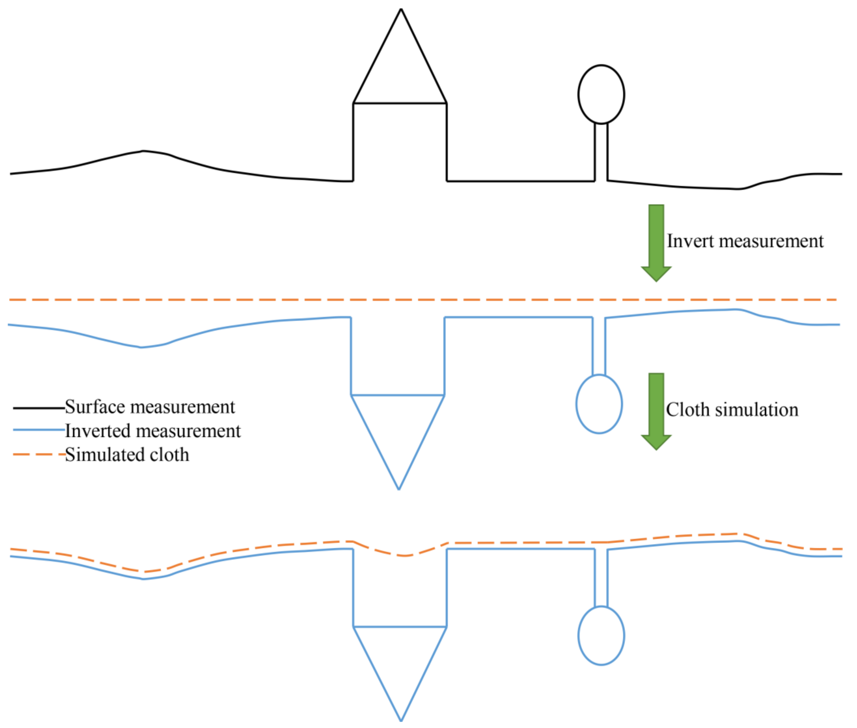
2.2. CSF for Ground Seed Selection

In the proposed method, the CSF algorithm is adapted to select the initial ground seeds instead of the local minimum points algorithm used by previous surface interpolation-based methods. The cloth simulation algorithm models cloth by simulating the physical process of cloth touching an entity in 3D computer graphics. The mass-spring model is a common method for cloth modeling. In the CSF algorithm, first, a piece of flexible cloth is covered above inverse surface measurement points. Then, this cloth drops down due to gravity until it fastens to the inverse landscape. The final fastened cloth is used as an approximated terrain surface to separate ground points and nonground points from point clouds [52], and the process is shown in Figure 1. The CSF algorithm mainly consists of three input parameters: grid resolution ($gr$), which represents the grid resolution of particles simulating the cloth and is closely related to the point spacing of the ALS point clouds; rigidity ($ri$) with a value of 1, 2 or 3, controls the rigidity (internal force) of the cloth particles; and slope post-processing factor ($st$) with a bool value, indicates whether or not slope terrain requires post processing. The CSF algorithm can generate a fine initial terrain, but it easily causes misclassification when further refining for the complex terrain. Therefore, the advantage of CSF is applied to select initial seeds for the interpolation-based filtering method.

The local minimum points algorithm is used by previous interpolation-based methods to obtain initial ground seeds. As a result, only a few points are selected as ground seed, which cause a low accuracy initial interpolation surface. In contrast, the CSF algorithm, with easy-to-set Integer and Boolean parameters, is easily used to select ground seeds. More importantly, it can provide a majority of valid ground seeds, which means that the selected seeds are actual ground points. Obviously, the more valid seeds that are used as control points (observed points), the higher the accuracy of the initial TPS interpolation surface is, which will improve the residual accuracy and filtering results. After the aforementioned outlier removal process is completed, the CSF algorithm is used to improve the initial seed accuracy of the ground points. Because the CSF algorithm is only used to select seeds, in consideration of efficiency and accuracy, a rigid cloth is able to generate enough ground seeds. Therefore, the rigidity is set to $ri=3$ in this study. In addition, in consideration of the point cloud density, the grid resolution $gr$ of the cloth is set to the provisional DEM grid resolution of the bottom hierarchy level. Regarding the slope post-processing factor $st$, for selecting more valid seeds at slope terrain, this parameter is set to true for slope terrain, otherwise it is set to false.

2.3. Local TPS Surface Interpolation Using Kdtree

An interpolation-based filtering method distinguish ground points from LiDAR data by using the elevation residuals between unclassified points and the interpolated raster surface. The TPS interpolation is a type of polyhedral function that approximates land surface. The resulting smooth surface is able to resist the effects of noise outliers during interpolation. For ground filtering, TPS interpolation is a better interpolator than other interpolation methods, such as ordinary kriging, inverse distance weighting and triangulated irregular network (TIN) [23]. This is because there are many holes in the point clouds that are iteratively filtered out nonground points, and the smoothness of TPS interpolation reduces the distortion of estimates at the regions of these holes compared with other interpolation methods mentioned above.

The TPS is a spline-based smoothing technique. It is also suited for interpolating large-scale geospatial data. In 3D space, given a series of control points $\left(x_i,y_i,z_i\right), i=1,2,\dots n$ in the spatial region, TPS interpolation is the solution for finding a continuous and smooth surface $f\left(x,y\right)$ by minimizing the bending energy function $E_f$ [22,58].

$$E_f=\iint \left[{\left(\frac{{\partial }^{2}f}{\partial x^2}\right)}^2+2{\left(\frac{{\partial }^{2}f}{\partial x\partial y}\right)}^2+{\left(\frac{{\partial }^{2}f}{\partial y^2}\right)}^2\right]dx\hspace{0.17em}dy$$

(2)

The interpolation of discrete points from the TPS surface is explicitly expressed as follows [59]:

$$f\left(x,y\right)={\displaystyle \sum }_{i=1}^{N}q\left(r_i\right)w_i+p\left(x,y\right)a$$

(3)

$${\displaystyle \sum }_{i=1}^N{w}_{i}p\left(x_i,y_i\right)=0$$

(4)

where $N$ is the number of control points used for TPS interpolation; $p\left(x,y\right)=1+x+y$ is the polynomial trend function for denoting surface variations and $a$ is its coefficient; $w_i$ is a weight related to the control points; $q\left(r_i\right)$ is a radial basis function with a radius $r_i=\Vert \left(x_i,y_i\right)-\left(x,y\right)\Vert$. In addition, for a TPS, this kernel function is defined as:

$$q\left(r\right)=r^2\mathit{ln}\left(r\right)$$

(5)

Based on Equations (3) and (4), the TPS surface can be estimated by solving the following linear system:

$$\left(\begin{array}{cc}Q& P\\ P^T& 0\end{array}\right)\left(\begin{array}{c}W\\ a\end{array}\right)=\left(\begin{array}{c}f\\ 0\end{array}\right)$$

(6)

where $Q$ is an $N\times N$ matrix defined by $q\left(r\right)$ at the control points; $P$ is an $N\times 3$ matrix defined by $p\left(x,y\right)$ at the control points; and $f$ denotes the observed values of the control points.

Because TPS computation has $\mathrm{O}\left(N^3\right)$ time complexity with inverse matrix operations and the interpolation process requires $\mathrm{O}\left(N^2\right)$, TPS interpolation is a computationally demanding method. As a result, global TPS interpolation using the total number of control points is computationally expensive, and oversmoothing the interpolation surface will result in missed terrain details. The proposed method employs a local TPS interpolation method, where only the local nearest neighbors are used for surface estimation. A KDtree index for the sample points is constructed to search for nearest neighbors quickly in dense point clouds. This TPS surface interpolation approach is very fast due to the optimization process with local neighbors using the KDtree index. In this paper, the number of neighbors used for estimating the surface is 16. Moreover, in practice, smoothing factor controls the smoothness of TPS interpolation.

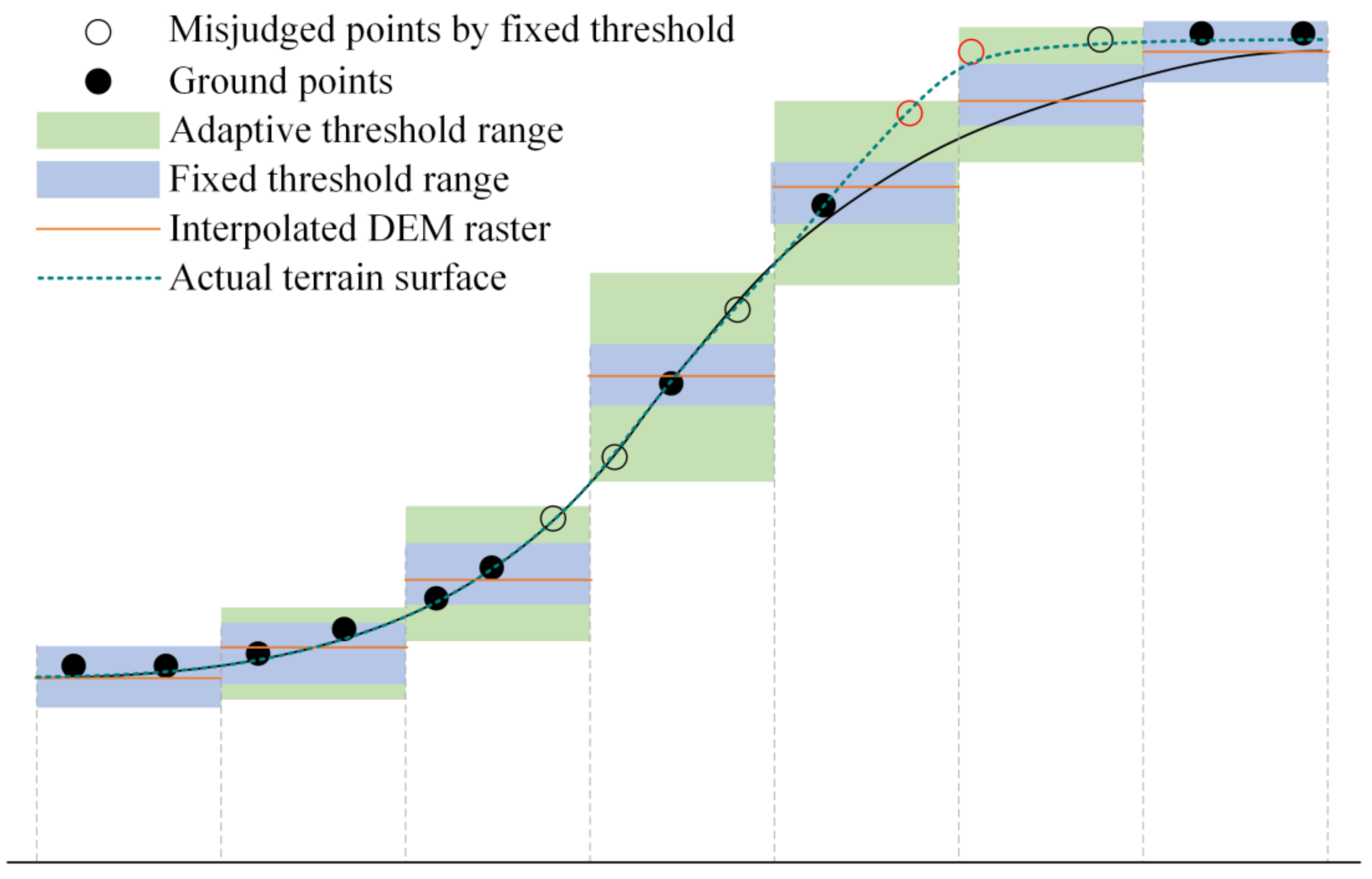
2.4. Relief Amplitude for Threshold Adaption

For the interpolation-based filtering method, elevation residual thresholds are used to distinguish between ground and nonground points obtained from ALS point clouds. The nine elevation residuals between the TPS-interpolated provisional DEM and the sample points, which are from $3\times 3$ neighbors for each cell, are used to distinguish ground points via comparison with the thresholds. In this way, the distinguishing result avoids distortion in only one residual [21]. Therefore, constructing adaptive residual thresholds by relief amplitude against each point is able to capture terrain detail features and significantly improve the accuracy of the ground filter in diverse terrains.

On steep slopes and in other areas with large height differences, the ground points are easily classified as nonground points by previously developed interpolation-based methods. This is mainly due to rough settings for the residual threshold. In this article, the relief amplitude is used to adaptively adjust residual thresholds by using terrain features. The relief amplitude is the difference between the highest and lowest elevations within a given area, as shown in Figure 2. The relief amplitude (as a terrain index) can depict the ruggedness of regional terrain, which reflects terrain complexity [55]. It is also able to quantitatively characterize landform features [60]. The relief amplitude is suitable for tuning elevation residual thresholds because of its simplicity of elevation expression and rich topographic content. The neighborhood analysis (window analysis for raster) method is applied for calculating the relief amplitude of the raster DEM [61]. Because the relief amplitude is a regional terrain index, its calculation should consider the scale. That is, the window size of the neighborhood analysis affects the calculation accuracy of the relief amplitude. Corresponding to the aforementioned nine elevation residuals, a $3\times 3$ window is used to calculate the relief amplitude of each cell in the raster DEM. In this paper, the mean relief amplitude is used, and the mean relief amplitude is defined as Equation (7):

$$r{a}_i=\mathit{Mean}\left(\mathit{Max}\left(H\left(n_i\right)\right)-\mathit{Min}\left(H\left(n_i\right)\right)\right)$$

(7)

where $H$ is elevation value of cell; $n_i$ is the $3\times 3$ neighbor cells for cell $i$.

Then, the residual thresholds $Z{t}_i$ of each cell can be defined as:

$$Z{t}_i=t+\mathit{deltat}+r{a}_i$$

(8)

where $t$ is the initial residual threshold; $\mathit{deltat}$ is the scale parameter, which increases with the increase in the hierarchy level; and $r{a}_i$ is the mean relief amplitude of each cell.

During filtering, from the top to the bottom hierarchy level, the scale parameter $\mathit{deltat}$ gradually increases for alleviating the scale effect of the method. At the same time (as shown in Figure 3), the relief amplitude is able to deal with complex terrain such as steep slopes. Because of using fixed threshold, some ground points are misjudged as nonground points on steep slopes (the circle points). In contract, the adaptive residual thresholds constructed by the relief amplitude can compensate residual threshold on steep slopes (the greed threshold range), which is able to alleviates this problem especially on the edge (the red circle points).

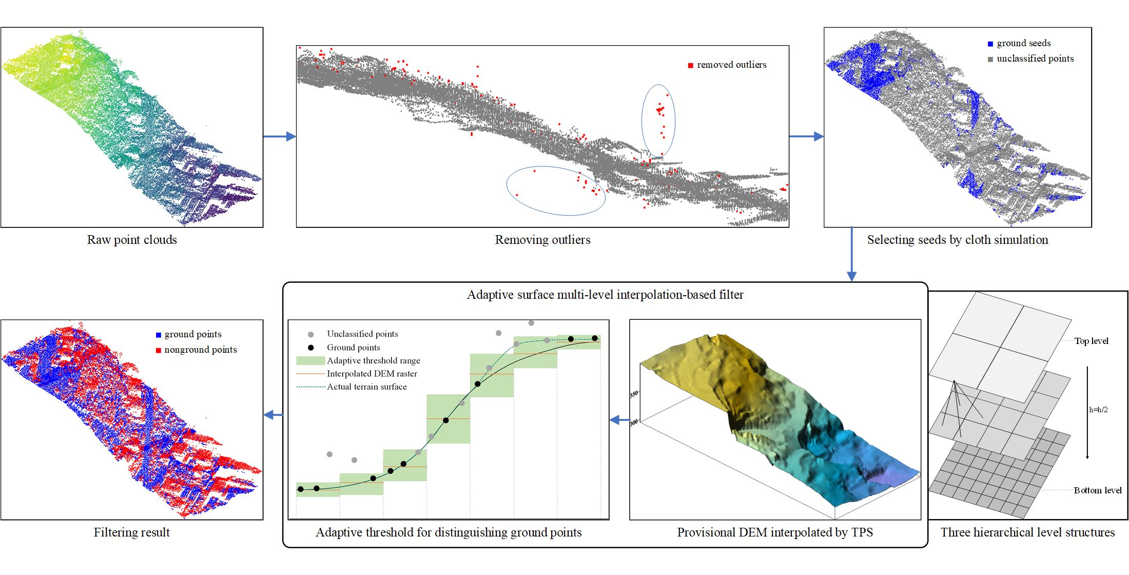
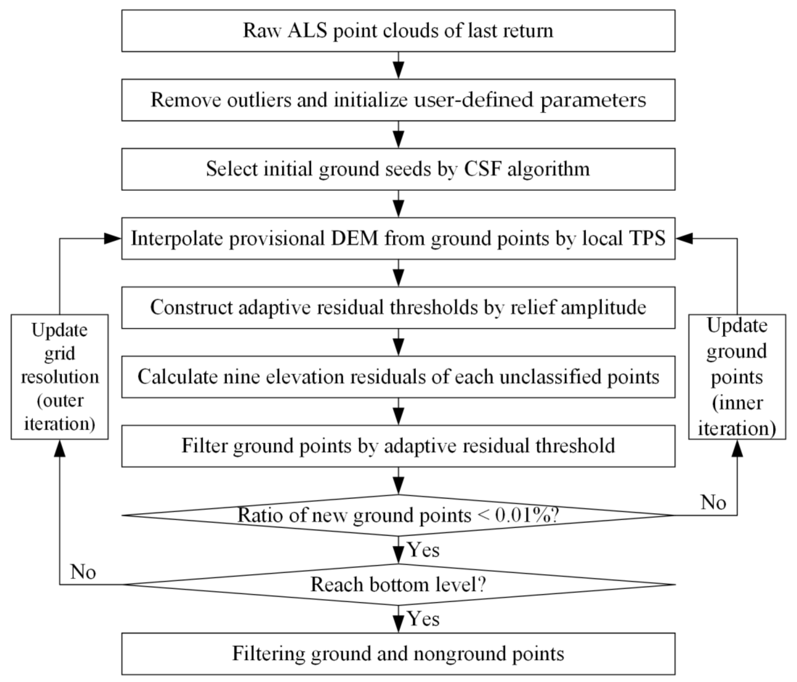
2.5. Adaptive Surface Interpolation Filter

The proposed method is an adaptive surface interpolation filter based on cloth simulation and relief amplitude. In this article, the ASI filter consists of three hierarchy levels. The algorithm includes an outer iterative process and an inner iterative process. The outer iterative process travels across all three hierarchy levels. Traveling from the top to the bottom hierarchy level, the provisional DEM grid resolution increases with a step of 2. The scale parameter $\mathit{deltat}$ constantly increases from 0.1 to 0.3 m to distinguish more ground points, and the smoothing factor $s$ constantly decreases from 0.3 to 0.1 to produce a better fitting surface. The grid resolution of the CSF is set to the bottom-level (finer) provisional DEM grid resolution in order to select a majority of valid seeds, which is able to guarantee the accuracy of the initial interpolated terrain surface. At the top level of the hierarchy, the selected ground seeds are used as control points for subsequent TPS interpolation. In the inner iterative process, the provisional raster DEM is interpolated from the ground points by local TPS interpolation. Therefore, the relief amplitude derived from the DEM is used to construct the adaptive residual thresholds. Then, the ground points are separated from unclassified points by comparisons between the elevation residuals of sample points and the adaptive residual threshold. Later, the ground and unclassified points are updated for the iteration of next hierarchy level. The ASI filter requires only three parameters to be user-defined: the initial grid resolution $h$, the initial residual threshold $t$ and the slope post-processing factor $st$; and the initial grid resolution $h$ is usually related to the point spacing of the ALS data.

The detailed filtering procedure of the proposed ASI is as follows (Figure 4):

(1)

Removing outliers from the raw ALS point clouds by SOR and initializing three user-defined parameters $h$, $t$ and $st$.

(2)

Initial ground seeds are selected from the point clouds without outliers by using the CSF algorithm, and the ground and unclassified points are updated.

(3)

The ground points are used to interpolate the provisional DEM raster surface by a TPS with a grid resolution $h$ and a smoothing factor $s$.

(4)

The mean relief amplitude $ra$ is computed from the provisional DEM, and the adaptive residual thresholds $Zt$ is constructed.

(5)

The elevation residuals $Zr$ are calculated from the unclassified points to corresponding nine neighbor cells of the provisional DEM.

(6)

The ground points are separated from the unclassified points if at least 4 of 9 $Zr$ values are smaller than the adaptive residual thresholds $Zt$. In addition, the ground and unclassified points are updated.

(7)

Steps (3)–(6) are repeated until the new ground points are less than a certain number.

(8)

Steps (3)–(7) are repeated in the next hierarchy level with updating grid resolution $h=h/2$ and scale parameter $\mathit{deltat}=\mathit{deltat}+0.1$. This outer iterative process terminates until the bottom hierarchy level is reached and the remaining unclassified points are labeled as nonground points.

3. Results

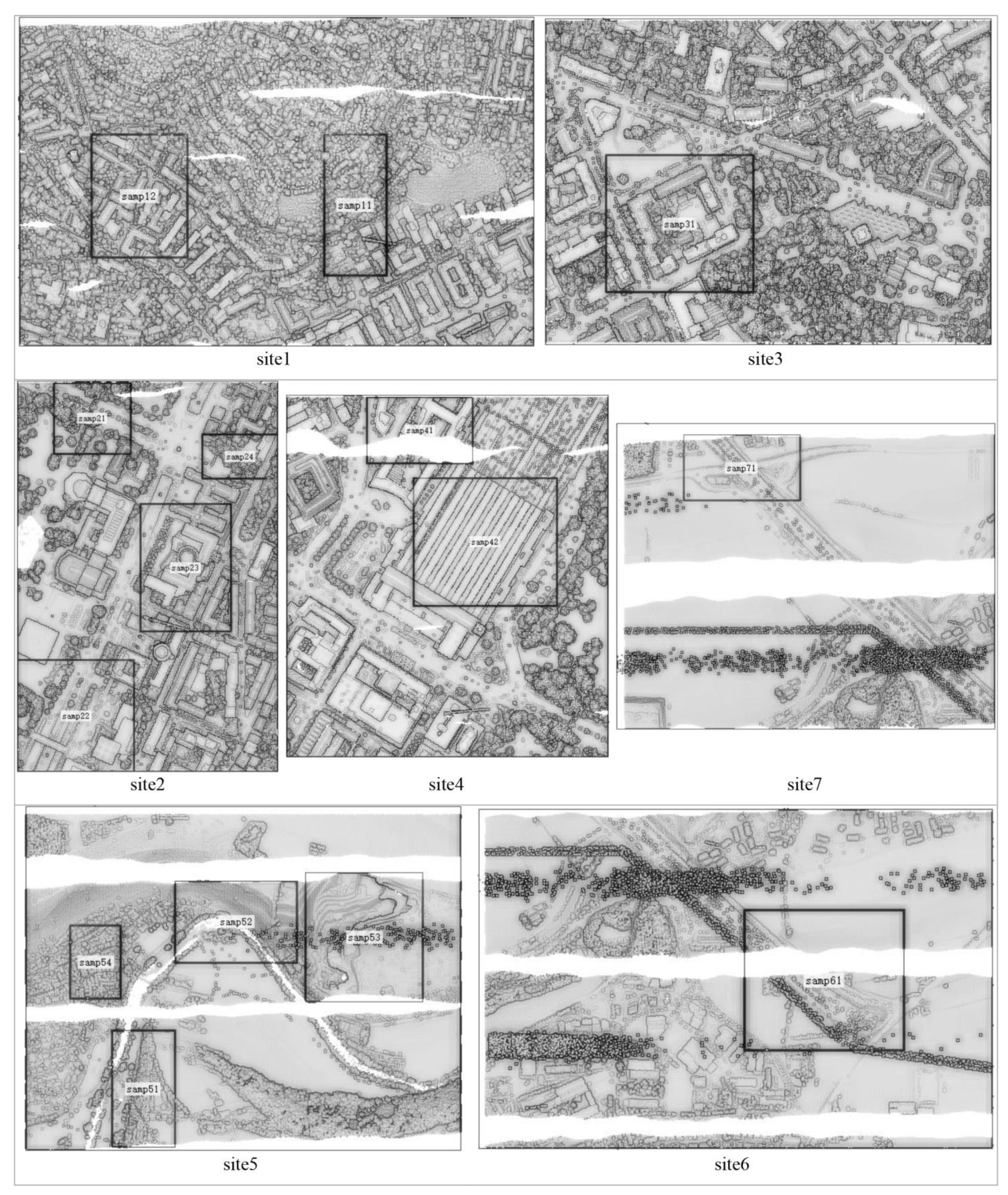
3.1. Experimental Data

To evaluate the performance of the proposed method, this paper used a benchmark dataset provided by the International Society for Photogrammetry and Remote Sensing (ISPRS) Working Group III/3. This benchmark dataset was gathered with an Optech ALTM scanner that scanned over an area containing the Vaihingen/Enz test field and the Stuttgart city center. The benchmark dataset consists of urban and rural groups with a total of 15 samples. The locations of the 15 samples on the corresponding seven sites are shown in Figure 5 and their relevant characteristics are shown in

Table 1. Characteristics of all study samples.

Region	Spacing	Site	Sample	Features
Urban	1–1.5 m	1	samp11	Mixture of vegetation and buildings on hillside
			samp12	Mixture of vegetation and buildings
		2	samp21	Road with bridge
			samp22	Irregularly shaped buildings and bridge
			samp23	Large, irregularly shaped buildings
			samp24	Steep slopes with vegetation
		3	samp31	Complex buildings
		4	samp41	Data gaps and irregularly shaped buildings
			samp42	Railway station with trains
Rural	2–3.5 m	5	samp51	Mixture of vegetation and buildings on hillside
			samp52	Steep, terraced slopes
			samp53	Steep, terraced slopes
			samp54	Irregularly shaped buildings
		6	samp61	Data gaps, discontinuity
		7	samp71	Underpass and bridge

. Moreover, the reference data for each sample were generated by manual filtering with knowledge of the landscape and aerial imagery, and each point in the samples was classified as a ground or nonground point [62].

3.2. Performance Measurement

The filtering of ground and nonground points from ALS data is a binary classification process. To quantitatively measure the performances of ground filtering algorithms, four indexes are used: the Type I error (T.I), Type II error (T.II), Total Error (T.E.) and kappa coefficient. The Type I error, also called the omission error, is equal to the number of ground points mistakenly classified as nonground points divided by the actual number of ground points. The Type II error, also called the commission error, is equal to the number of nonground points mistakenly classified as ground points divided by the actual number of nonground points. The T.E. is equal to the sum of all mistakenly classified points divided by the total number of points in the dataset. Cohen’s kappa coefficient measures the overall agreement between two judges while considering the possibility of the agreement occurring by chance [63]. The kappa coefficient ranges from negative 1 to positive 1, with negative 1 indicating strong disagreement, zero indicating opportunistic agreement, and positive 1 indicating strong agreement. These four metric indexes can be calculated by the cross matrix shown in

Table 2. The cross matrix between the reference results and ground filtered results.

	Filtered	Ground	Nonground
References
ground		a	b	f = (a + b)/e
nonground		c	d	g = (c + d)/e
		h = (a + c)/e	i = (b + d)/e	e = a + b + c + d

[62]. These four metric indexes are calculated using the following equations:

$$T.I=\frac{b}{a+b}$$

(9)

$$T.II=\frac{c}{c+d}$$

(10)

$$T.E.=\frac{b+c}{a+b+c+d}$$

(11)

$$P_o=\frac{a+d}{e}$$

(12)

$$P_e=f\ast h+g\ast i$$

(13)

$$\mathit{Kappa}=\frac{P_o-P_e}{1-P_e}$$

(14)

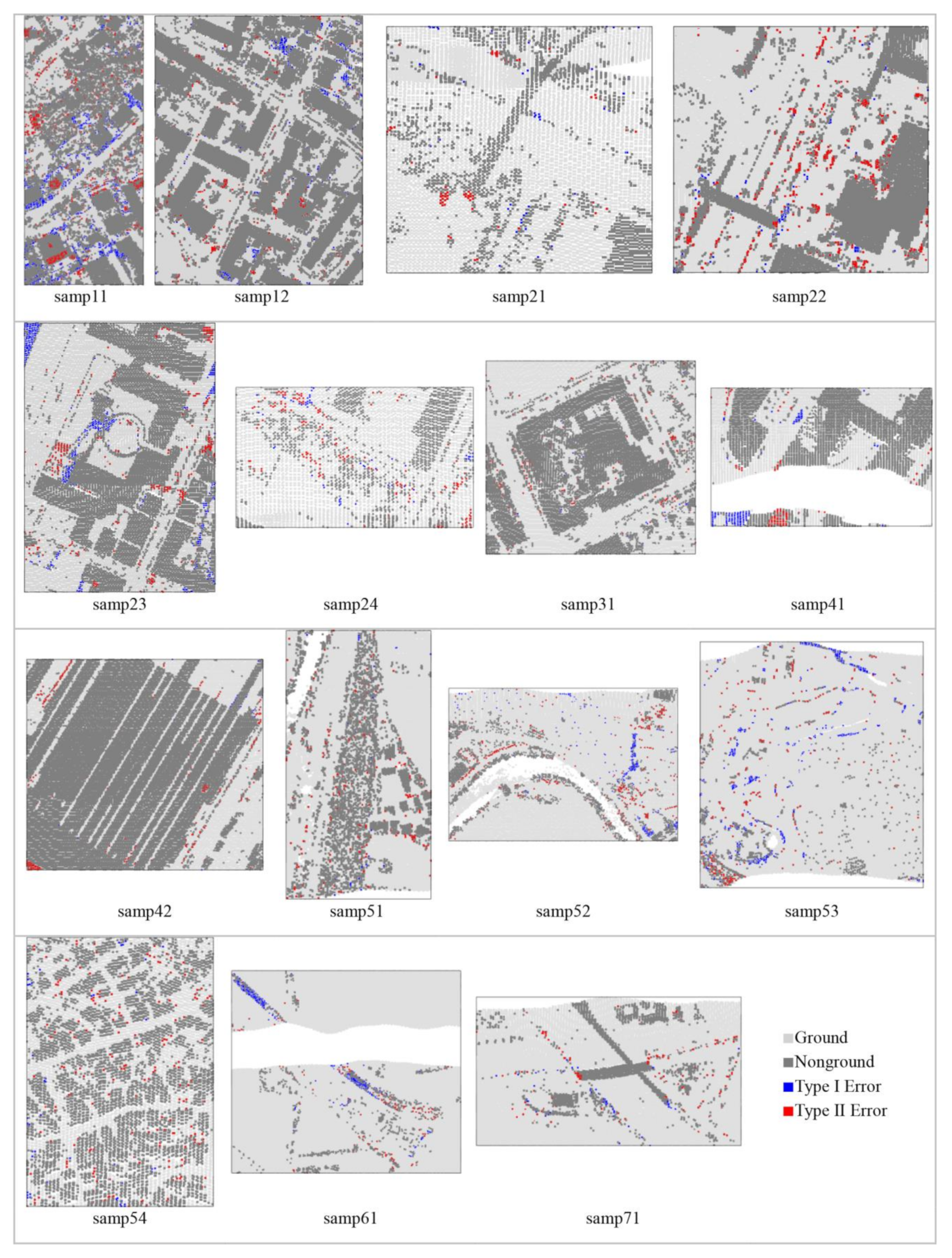
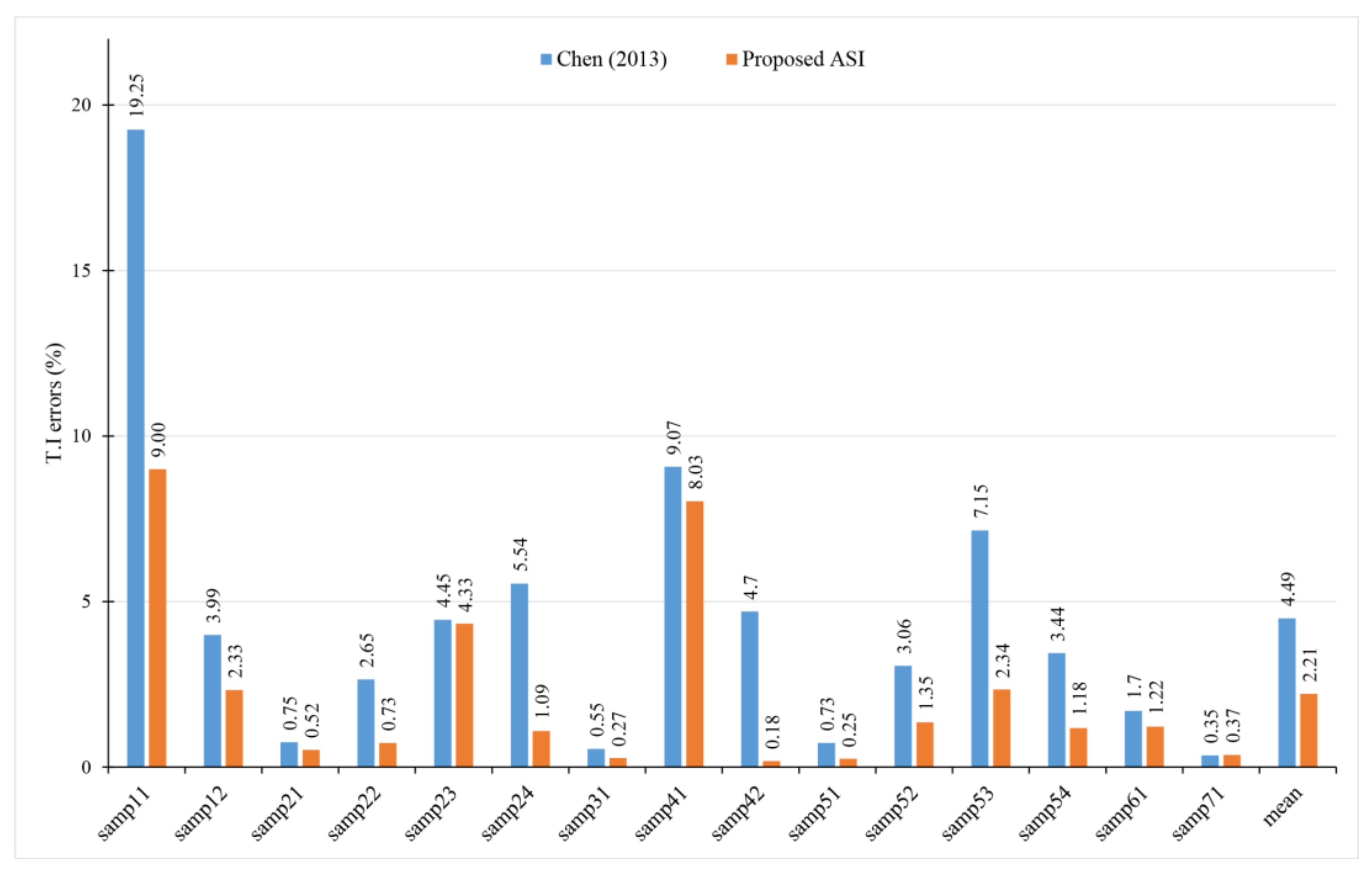
3.3. Results and Analysis

The proposed ASI method only has three user-defined parameters: the initial grid resolution $h$, the initial residual threshold $t$ and the slope post-processing factor $st$. The initial parameter configurations are shown in

Table 3. The initial grid resolution and residual threshold used in the ASI procedure.

Sample	h (m)	t (m)	st (Bool)
samp11	2	0.2	False
samp12	4	0	True
samp21	2	0	False
samp22	2	0.2	True
samp23	4	0.2	True
samp24	2	0.1	True
samp31	4	0	True
samp41	4	0.1	True
samp42	4	0.4	True
samp51	2	0.1	False
samp52	4	0.2	True
samp53	4	0.3	True
samp54	4	0.2	False
samp61	2	0.5	False
samp71	2	0.3	False

. This demonstrates that the initial grid resolution is 2 m or 4 m, which is slightly larger than the average point spacing of these ALS point clouds. The initial residual threshold $t$ ranges from 0.0 m to 0.5 m, and it is related to the surface undulation of the study area. The slope post-processing factor $st$ is set to true for slope terrain, otherwise it is set to false.

The accuracy error and kappa coefficient of the ASI filtering results against the fifteen samples of the ISPRS benchmark dataset are shown in

Table 4. Errors and kappa coefficients of the ASI filtering results for all samples.

Sample	T.I (%)	T.II (%)	T.E. (%)	Kappa (%)
samp11	9.00	12.93	10.68	78.16
samp12	2.33	2.91	2.61	94.77
samp21	0.52	3.17	1.10	96.79
samp22	0.73	7.72	2.91	93.10
samp23	4.33	4.70	4.50	90.97
samp24	1.09	9.62	3.43	91.21
samp31	0.27	2.00	1.07	97.85
samp41	8.03	5.22	6.62	86.75
samp42	0.18	1.28	0.96	97.70
samp51	0.25	6.62	1.64	95.09
samp52	1.35	16.38	2.93	84.07
samp53	2.34	23.11	3.18	64.49
samp54	1.18	4.04	2.72	94.55
samp61	1.22	12.19	1.60	78.27
samp71	0.37	7.23	1.15	94.16
mean	2.21	7.94	3.14	89.20
std	2.69	5.83	2.49	9.06

, and the error distribution is shown in Figure 6. Table 4 demonstrates that the proposed ASI method has very high performance and very low T.I errors. In particular, six samples, including samp21, samp22, samp31, samp42 samp51 and samp71, obtain T.I errors less than 1% and kappa coefficients greater than 90%. The results also illustrate that eight samples with fine precision, including samp12, samp21, samp22, samp31, samp42, samp51, samp54 and samp71, obtain T.E. values less than 3% and kappa coefficients greater than 90%. This is because the above eight sample areas are all relatively flat. These results are similar to those of previous interpolation-based methods, which perform well in flat areas but poorly in steep slope terrains [54]. Unfortunately, the T.II errors are slightly high for several samples. Only samp11 has a T.E. greater than 10% (10.68%), with a high T.II error rate of 12.93%. This is because many of the buildings in samp11 are situated on slopes that are easily misjudged. Furthermore, there is much low vegetation on the slope that has been recognized as a ground point. Samp41 also has weak accuracy due to some missing data and the presence of many confusing outliers in this sample. As a result, removing outliers is a critical step of filtering preprocessing. Regarding the kappa coefficient, the proposed method has good performance, with a mean kappa coefficient reaching 89.20%. Moreover, ten samples obtain kappa coefficients greater than 90%. However, the method achieves weak filtering results for samp53 (64.49%) because of discontinuous terrain features with steep regions and terraces in this sample. To preserve more terrain details, some points of low vegetation are accepted as ground points, resulting in a high T.II error of 23.11%.

To evaluate the performance of the proposed method, this paper compares the filtering results of the proposed method to those of four other interpolation-based methods, all of which are tested against the ISPRS benchmark dataset. The T.E. comparison is shown in

Table 5. Comparison between the T.E. values (%) of the proposed method and other interpolation-based methods. (The best results across all the methods at each sample are highlighted in bold.)

Sample	Mongus (2012)	Chen (2013)	Meng (2019)	Li (2020)	Proposed ASI
samp11	11.01	13.01	10.20	9.44	10.68
samp12	5.17	3.38	2.97	3.34	2.61
samp21	1.98	1.34	1.35	1.50	1.10
samp22	6.56	4.67	3.82	4.93	2.91
samp23	5.83	5.24	5.03	4.42	4.50
samp24	7.98	6.29	5.22	6.87	3.43
samp31	3.34	1.11	2.13	1.39	1.07
samp41	3.71	5.58	6.40	4.82	6.62
samp42	5.72	1.72	0.66	0.81	0.96
samp51	2.59	1.64	1.71	1.79	1.64
samp52	7.11	4.18	3.39	3.47	2.93
samp53	8.52	7.29	6.58	5.96	3.18
samp54	6.73	3.09	2.93	2.95	2.72
samp61	4.85	1.81	2.10	1.69	1.60
samp71	3.14	1.33	1.34	1.60	1.15
mean	5.62	4.11	3.72	3.67	3.14
std	2.39	3.06	2.48	2.35	2.49

and the kappa coefficients are shown in

Table 6. Comparison between the kappa coefficients (%) of the proposed method and other interpolation-based methods. (The best results across all the methods at each sample are highlighted in bold.)

Sample	Mongus (2012)	Chen (2013)	Meng (2019)	Li (2020)	Proposed ASI
samp11	77.31	74.12	79.09	80.74	78.16
samp12	89.66	93.23	94.05	93.31	94.77
samp21	94.09	96.10	96.02	95.62	96.79
samp22	84.74	89.03	91.05	88.35	93.10
samp23	88.29	89.49	89.92	91.12	90.97
samp24	80.07	84.53	86.86	82.78	91.21
samp31	93.25	97.76	95.69	97.21	97.85
samp41	92.61	88.83	87.19	90.36	86.75
samp42	86.95	95.81	98.42	98.06	97.70
samp51	92.18	95.17	94.89	94.66	95.09
samp52	68.45	78.91	82.82	82.42	84.07
samp53	42.18	46.69	49.12	43.43	64.49
samp54	86.63	93.90	94.11	94.08	94.55
samp61	65.05	77.36	74.82	77.81	78.27
samp71	85.04	93.19	93.33	92.08	94.16
mean	81.77	86.27	87.16	86.80	89.20
std	13.50	12.72	12.05	13.08	9.06

. Generally, the proposed method performs well on the experimental data, with the lowest mean T.E. (3.14%) and the highest mean kappa coefficient (89.20%). Compared to the other four methods, the proposed method obtains the lowest T.E. values for ten samples: samp12, samp21, samp22, samp24, samp31, samp52, samp53, samp54, samp61 and samp71. At the same time, these ten samples yield the highest kappa coefficients, which confirms the reliability of the proposed method. Furthermore, the T.E. values for the remaining samples are comparable to those of other interpolation-based methods. In the areas with many buildings on flat terrain, such as samp12, samp24, samp31 and samp54, the ground and objects are precisely distinguished. This is because enough valid seeds are derived from the proposed method to reconstruct a high-quality initial topographic surface, which is conducive to the separation of building objects. In areas of discontinuous terrain with steep slopes, such as samp52 and samp53, the ground points on the steep slopes are clearly distinguished. The reason for this is that the proposed method applies relief amplitude to construct the adaptive residual thresholds for filtering, which is capable of capturing the detailed topographic characteristics of steep regions and terraces. Especially for samp53 with steep and terraced slopes, the proposed method obtains a much lower T.E. and a much higher kappa coefficient than those of the other interpolation-based methods. This illustrates that the proposed filtering method is able to preserve steep slope terrain by introducing relief amplitude.

The proposed method improves the multiresolution hierarchical classification (MHC) algorithm [21] by means of the CSF algorithm [52] and the introduction of relief amplitude. To analyze the improvement yielded by the proposed method, the T.E. values of the filtering results obtained against each sample by the proposed method, the MHC algorithm, the CSF algorithm and another improved progressive TIN densification (PTD) method using a CSF [64], are compared, as shown in

Table 7. Comparison between the T.E. values (%) of the proposed method and the inspired methods. (The best results across all the methods at each sample are highlighted in bold.)

Sample	Chen (2013)	Zhang (2016)	Cai (2019)	Proposed ASI
samp11	13.01	12.01	16.24	10.68
samp12	3.38	2.97	8.85	2.61
samp21	1.34	3.42	14.18	1.10
samp22	4.67	8.94	4.25	2.91
samp23	5.24	4.79	8.52	4.50
samp24	6.29	2.87	15.59	3.43
samp31	1.11	1.61	7.28	1.07
samp41	5.58	5.14	13.04	6.62
samp42	1.72	1.58	4.75	0.96
samp51	1.64	3.08	3.51	1.64
samp52	4.18	3.93	4.65	2.93
samp53	7.29	5.20	3.95	3.18
samp54	3.09	3.18	2.58	2.72
samp61	1.81	1.49	0.86	1.60
samp71	1.33	5.71	2.03	1.15
mean	4.11	4.39	7.35	3.14
std	3.06	2.76	4.98	2.49

. Compared with the MHC method, the proposed method obtains lower T.E. values in samples other than samp41 because the proposed method acquires many valid ground seeds, further integrating terrain information. Regarding samp41, because of missing data and confusing outliers, the calculated relief amplitude has difficulty expressing the actual terrain. This causes the proposed method to have a slightly low filtering accuracy, with a slightly high commission error. Even in comparison with the fine PTD method improved by the use of a CSF, the proposed method shows great performance, where eleven samples, samp11, samp12, samp21, samp22, samp23, samp31, samp42, samp51, samp52, samp53 and samp71, yield the lowest T.E. values. Particularly in the slope areas of samp22, samp52 and samp53, the gentle and steep slope regions are precisely distinguished. This illustrates that the PTD method using a CSF for seed selection is not able to obtain good accuracy, but it can be used for the proposed hierarchical interpolation method integrated with the CSF algorithm. The results show that the proposed method improves upon the filtering accuracy of previously developed methods, especially in terrain with steep slopes.

4. Discussion

4.1. Performance of Seed Selection Strategy

The hierarchical surface interpolation filter accumulates errors when iteratively interpolating the provisional DEM surface. Therefore, the accuracy of the initial provisional surface is critical for optimizing the filtering accuracy. The approximate precision between the interpolated provisional DEM surface and the actual terrain surface depends on the initially selected ground seeds. As a result, a high-quality topographic surface, constructed by sufficient valid initial seeds, significantly improves the filtering results in terms of distinguishing between ground and nonground points. To explore the effects of ground seed selection, the number and accuracy of initial seeds are used to indicate the performance of seed selection methods. The accuracy of the initial seeds is represented by the approximate precision of the initial DEM surface interpolated by the seeds. This is measured by the root mean square error (RMSE) between the initial DEM surface interpolated by seeds and the true ground point elevation; the RMSE can be calculated as follows:

$$\mathit{RMSE}=\sqrt{\frac{{{\displaystyle \sum }}_{i=1}^n{\left(Z_i^{’}-Z_i\right)}^2}{n}}$$

(15)

where $\mathrm{Z}$ denotes the elevation values of true ground points, $Z^{\prime }$ denotes the elevation values of the interpolated DEM surface at the locations of the true ground points, $\mathrm{i}$ denotes the ith true ground point, and n denotes the total number of true ground points.

The RMSE and number of seeds obtained for each sample by the proposed ASI method are compared with those achieved by Chen’s MHC method, and the comparison results are shown in

Table 8. Comparison between the RMSE and number of seeds obtained for each sample by Chen’s MHC method and the proposed ASI method. (The best RMSE results across all the methods at each sample are highlighted in bold.)

Sample	MHC		Proposed ASI
	Points	RMSE (m)	Points	RMSE (m)
samp11	55	3.17	9322	3.53
samp12	63	1.66	24,233	0.99
samp21	20	0.55	9561	0.11
samp22	49	2.01	21,668	0.43
samp23	35	3.56	11,196	1.47
samp24	28	2.26	5016	0.60
samp31	81	0.73	15,449	0.17
samp41	24	3.50	4688	1.67
samp42	56	0.85	11,119	0.54
samp51	120	1.10	11,927	0.51
samp52	346	1.91	13,827	3.07
samp53	500	4.54	21,594	5.74
samp54	140	0.60	2061	0.92
samp61	516	1.37	26,460	1.26
samp71	108	2.17	8489	1.57
mean	143	2.00	13,107	1.51

. The results show that the MHC method generates an average of 143 ground seeds from the 15 samples. The proposed ASI method generates an average of 13,107 ground seed points, which indicates that this approach can significantly increase the number of ground seed points. At the same time, the proposed method obtains a lower mean RMSE of 1.51, which ensures the accuracy of the selected seeds. These results also demonstrate that the proposed method produces many more seeds than does the MHC method for each sample. The results of the proposed method for eleven samples obtain lower RMSEs, and the results of the remaining samples are comparable to those of the MHC method with the exception of samp52. This is because the extended local minimum algorithm used by the MHC approach employs a large window that is larger than the largest object size in the study area, causing only a few points to be selected as seeds. The CSF algorithm used by the proposed method is able to acquire more points. Furthermore, a few seeds cannot be interpolated to produce a high-precision DEM surface. For samp52, the MHC method obtains a lower RMSE than that of the proposed method. This is because in samp52 with steep terrain, the MHC method, which uses a large window that covers the whole study area, is able to disperse the acquired seed points across the entire study area, thereby obtaining a good overall interpolation accuracy. For the CSF algorithm used by the proposed method, the selected seeds cluster in flat and gentle slope regions, while in steep slope regions can cause some misclassification. Nonetheless, for samp52, the proposed method obtains better filtering accuracy after performing the subsequent procedure. This confirms the advantage of the adaptive residual thresholds used by the proposed ground filter from another point of view.

To further demonstrate the performance of the seed selection strategy utilized in the proposed method, the samp51 with slopes and low vegetation is used to select seeds by the proposed method and the MHC approach. Then, the initial provisional DEM raster surface is interpolated by these seeds, and the results are shown in Figure 7. This illustrates that the initial DEM surface generated by the MHC method is quite smooth and loses terrain details because too few seeds are selected to generate a high-precision initial topographic surface. In contrast, the initial DEM surface produced by the proposed method is very close to the reference DEM surface and preserves most of the topographic characteristics because the CSF algorithm adopted by the proposed method generates a sufficient number of valid initial ground seeds.

4.2. Effect of Adaptive Residual Thresholds

Due to their use of fixed elevation residual thresholds, some previously developed interpolation-based methods result in low accuracy in terrain with steep slopes. The proposed method constructs adaptive elevation residual thresholds according to regional topographical characteristics by introducing relief amplitude. The relief amplitude is used to delicately construct adaptive residual thresholds to accurately distinguish between ground points in steep terrain. Hence, this factor principally contributes to reducing the omission error of the results. Therefore, to explore the filtering performance of the proposed method, the T.I errors for each sample obtained by Chen’s MHC method and the proposed ASI method are compared, and the results are shown in Figure 8. The results show that the proposed method obtains a lower mean T.I error than the MHC method. For each sample, the proposed method obtains a lower T.I error than the MHC method, aside from samp71, which yields similarly low T.I errors. This illustrates that the proposed method significantly reduces the omission error. This is because the adaptive residual thresholds employed by the proposed method can capture more topographic characteristics and prevent points in these areas from being missed.

To further demonstrate the effect of the adaptive residual thresholds used by the proposed method for discontinuous terrain with steep slopes, samp53 with steep slopes and terraces is filtered by the proposed method, the MHC method and the CSF algorithm. The error distributions of the different filtering results are shown in Figure 9. This demonstrates that the CSF method has poor filtering accuracy, and it has very high T.I errors in steep regions and even in flat regions. The reason for this phenomenon is that the sample has a sunken topography with steep slopes and terraces, which limits the accuracy of cloth simulation results when utilizing rigid cloths. In comparison with that of the MHC method, the regions in black boxes indicate that the proposed method improves the filtering accuracy for this sample. That is, the T.I error risk of misclassifying ground points as nonground points is reduced. The regions of improved accuracy are concentrated in break lines and steep slopes. The MHC method uses only a fixed elevation residual threshold; thus, it is vulnerable to misclassifying ground points in steep slope areas and yielding higher T.I error rates. However, the proposed method uses the adaptive residual thresholds constructed based on the relief amplitude of the local terrain to improve the classification outputs. As a result, the filtering threshold must be compensated for greatly to correctly accept points on the edges of break lines as ground points. The results indicate that the adaptive residual thresholds of the proposed method improve the filtering accuracy in regions with steep slopes, break lines and terraces.

5. Conclusions

Ground filtering is an essential step of most applications involving ALS point clouds. Interpolation-based filtering algorithms have been proven to be powerful and efficient, especially in forest areas. However, such methods easily cause misjudgments in steep terrain. To enhance the robustness and accuracy of interpolation-based filtering algorithms, this paper proposes an improved adaptive surface interpolation method with a multilevel hierarchy by using cloth simulation and relief amplitude. The proposed method integrates the CSF algorithm to select sufficient valid initial ground seeds for generating high-quality topographic surfaces. It also introduces relief amplitude for the consideration of complex terrain features; this is done to delicately construct adaptive residual thresholds for accurately distinguishing the ground points of ALS data. In addition, local TPS interpolation using the KDtree index improves the accuracy and efficiency of the interpolation process. The conducted experiment tests the performance of the proposed method against the benchmark dataset provided by the ISPRS. In contrast with other interpolation-based algorithms, the proposed method significantly improves both the overall accuracy and kappa coefficient of the obtained results. This demonstrates that the proposed method has higher filtering accuracy than these competing approaches. Optimized initial ground seeds and adaptive residual thresholds contribute to very low T.I error rates. In terms of T.E., for the fifteen samples, the proposed method obtains the best filtering results in rural environments with complex terrain containing steep slopes and break lines. Although our method achieves a great filtering effect, it is still a great challenge to accurately distinguish ground points in large complex areas with many outliers. The proposed ASI method still has slightly high commission errors for some samples. Future works will focus on integrating the waveform and spectrum information of airborne LiDAR systems into the filtering process to reduce the commission error and improve the applicability of the proposed filter by accurately identifying areas with very low vegetation and buildings.

References

1. Chen, Z.; Gao, B.; Devereux, B. State-of-the-Art: DTM Generation Using Airborne LIDAR Data. Sensors 2017, 17, 150. [Google Scholar] [CrossRef] [PubMed] [Green Version]
2. Meng, X.; Currit, N.; Zhao, K. Ground Filtering Algorithms for Airborne LiDAR Data: A Review of Critical Issues. Remote. Sens. 2010, 2, 833–860. [Google Scholar] [CrossRef] [Green Version]
3. Chen, C.; Li, Y. A Fast Global Interpolation Method for Digital Terrain Model Generation from Large LiDAR-Derived Data. Remote Sens. 2019, 11, 1324. [Google Scholar] [CrossRef] [Green Version]
4. Tarolli, P. High-Resolution Topography for Understanding Earth Surface Processes: Opportunities and Challenges. Geomorphology 2014, 216, 295–312. [Google Scholar] [CrossRef]
5. Liu, X. Airborne LiDAR for DEM Generation: Some Critical Issues. Prog. Phys. Geogr. Earth Environ. 2008, 32, 31–49. [Google Scholar] [CrossRef]
6. Wang, R.; Peethambaran, J.; Chen, D. LiDAR Point Clouds to 3-D Urban Models: A Review. IEEE J. Sel. Top. Appl. Earth Obs. Remote. Sens. 2018, 11, 606–627. [Google Scholar] [CrossRef]
7. Wu, B.; Yu, B.; Wu, Q.; Yao, S.; Zhao, F.; Mao, W.; Wu, J. A Graph-Based Approach for 3D Building Model Reconstruction from Airborne LiDAR Point Clouds. Remote. Sens. 2017, 9, 92. [Google Scholar] [CrossRef] [Green Version]
8. Huang, H.; Brenner, C.; Sester, M. A Generative Statistical Approach to Automatic 3D Building Roof Reconstruction from Laser Scanning Data. ISPRS J. Photogramm. Remote. Sens. 2013, 79, 29–43. [Google Scholar] [CrossRef]
9. Fischer, F.J.; Labrière, N.; Vincent, G.; Hérault, B.; Alonso, A.; Memiaghe, H.; Bissiengou, P.; Kenfack, D.; Saatchi, S.; Chave, J. A Simulation Method to Infer Tree Allometry and Forest Structure from Airborne Laser Scanning and Forest Inventories. Remote. Sens. Environ. 2020, 251, 112056. [Google Scholar] [CrossRef]
10. Khosravipour, A.; Skidmore, A.K.; Isenburg, M. Generating Spike-Free Digital Surface Models Using LiDAR Raw Point Clouds: A New Approach for Forestry Applications. Int. J. Appl. Earth Obs. Geoinf. 2016, 52, 104–114. [Google Scholar] [CrossRef]
11. Khosravipour, A.; Skidmore, A.; Isenburg, M.; Wang, T.; Hussin, Y.A. Generating Pit-free Canopy Height Models from Airborne Lidar. Photogramm. Eng. Remote. Sens. 2014, 80, 863–872. [Google Scholar] [CrossRef]
12. Pfeifer, N.T.R.; Briese, C.; Rieger, W. Interpolation of High Quality Ground Models from Laser Scanner Data in Forested Areas. Int. Arch. Photogramm. Remote Sens. 1999, 32, 31–36. [Google Scholar]
13. Li, Y.; Wang, J.; Li, B.; Sun, W.; Li, Y. An Adaptive Filtering Algorithm of Multilevel Resolution Point Cloud. Surv. Rev. 2021, 53, 300–311. [Google Scholar] [CrossRef]
14. Meng, X.; Lin, Y.; Yan, L.; Gao, X.; Yao, Y.; Wang, C.; Luo, S. Airborne LiDAR Point Cloud Filtering by a Multilevel Adaptive Filter Based on Morphological Reconstruction and Thin Plate Spline Interpolation. Electronics 2019, 8, 1153. [Google Scholar] [CrossRef] [Green Version]
15. Cheng, P.; Hui, Z.; Xia, Y.; Ziggah, Y.Y.; Hu, Y.; Wu, J. An Improved Skewness Balancing Filtering Algorithm Based on Thin Plate Spline Interpolation. Appl. Sci. 2019, 9, 203. [Google Scholar] [CrossRef] [Green Version]
16. Hui, Z.; Li, D.; Jin, S.; Ziggah, Y.Y.; Wang, L.; Hu, Y. Automatic DTM Extraction from Airborne LiDAR Based on Expectation-Maximization. Opt. Laser Technol. 2019, 112, 43–55. [Google Scholar] [CrossRef]
17. Qin, L.; Wu, W.; Tian, Y.; Xu, W. LiDAR Filtering of Urban Areas with Region Growing Based on Moving-Window Weighted Iterative Least-Squares Fitting. IEEE Geosci. Remote. Sens. Lett. 2017, 14, 841–845. [Google Scholar] [CrossRef]
18. Zhao, X.; Guo, Q.; Su, Y.; Xue, B. Improved Progressive TIN Densification Filtering Algorithm for Airborne LiDAR Data in Forested Areas. ISPRS J. Photogramm. Remote. Sens. 2016, 117, 79–91. [Google Scholar] [CrossRef] [Green Version]
19. Su, W.; Sun, Z.; Zhong, R.; Huang, J.; Li, M.; Zhu, J.; Zhang, K.; Wu, H.; Zhu, D. A New Hierarchical Moving Curve-Fitting Algorithm for Filtering Lidar Data for Automatic DTM Generation. Int. J. Remote. Sens. 2015, 36, 3616–3635. [Google Scholar] [CrossRef]
20. Hu, H.; Ding, Y.; Zhu, Q.; Wu, B.; Lin, H.; Du, Z.; Zhang, Y.; Zhang, Y. An Adaptive Surface Filter for Airborne Laser Scanning Point Clouds by Means of Regularization and Bending Energy. ISPRS J. Photogramm. Remote. Sens. 2014, 92, 98–111. [Google Scholar] [CrossRef]
21. Chen, C.; Li, Y.; Li, W.; Dai, H. A Multiresolution Hierarchical Classification Algorithm for Filtering Airborne LiDAR Data. ISPRS J. Photogramm. Remote. Sens. 2013, 82, 1–9. [Google Scholar] [CrossRef]
22. Mongus, D.; Žalik, B. Parameter-Free Ground Filtering of LiDAR Data for Automatic DTM Generation. ISPRS J. Photogramm. Remote. Sens. 2012, 67, 1–12. [Google Scholar] [CrossRef]
23. Evans, J.; Hudak, A.T. A Multiscale Curvature Algorithm for Classifying Discrete Return LiDAR in Forested Environments. IEEE Trans. Geosci. Remote. Sens. 2007, 45, 1029–1038. [Google Scholar] [CrossRef]
24. Pfeifer, N.; Stadler, P.; Briese, C. Derivation of Digital Terrain Models in the SCOP++ Environment. In Proceedings of the OEEPE Workshop on Airborne Laserscanning and Interferometric SAR for Digital Elevation Models, Stockholm, Sweden, 1–3 March 2001. [Google Scholar]
25. Axelsson, P. Processing of Laser Scanner Data—Algorithms and Applications. ISPRS J. Photogramm. Remote. Sens. 1999, 54, 138–147. [Google Scholar] [CrossRef]
26. Kraus, K.; Pfeifer, N. Determination of Terrain Models in Wooded Areas with Airborne Laser Scanner Data. ISPRS J. Photogramm. Remote. Sens. 1998, 53, 193–203. [Google Scholar] [CrossRef]
27. Yang, Y.B.; Zhang, N.N.; Li, X.L. Adaptive Slope Filtering for Airborne Light Detection and Ranging Data in Urban Areas Based on Region Growing Rule. Surv. Rev. 2016, 1–8. [Google Scholar] [CrossRef]
28. Guan, H.; Li, J.; Yu, Y.; Zhong, L.; Ji, Z. DEM Generation from Lidar Data in Wooded Mountain Areas by Crosssection-Plane Analysis. Int. J. Remote. Sens. 2014, 35, 927–948. [Google Scholar] [CrossRef]
29. Susaki, J. Adaptive Slope Filtering of Airborne LiDAR Data in Urban Areas for Digital Terrain Model (DTM) Generation. Remote. Sens. 2012, 4, 1804–1819. [Google Scholar] [CrossRef] [Green Version]
30. Wang, C.K.; Tseng, Y.H. Dem Generation from Airborne Lidar Data by an Adaptive Dual-Directional Slope Filter. In Proceedings of the ISPRS TC VII Symposium—100 Years ISPRS, Vienna, Austria, 5–7 July 2010. [Google Scholar]
31. Meng, X.; Wang, L.; Silván-Cárdenas, J.L.; Currit, N. A Multi-Directional Ground Filtering Algorithm for Airborne LIDAR. ISPRS J. Photogramm. Remote. Sens. 2009, 64, 117–124. [Google Scholar] [CrossRef] [Green Version]
32. Sithole, G. Filtering of Laser Altimetry Data Using a Slope Adaptive Filter. Int. Arch. Photogramm. Remote Sens. 2001, 34, 203–210. [Google Scholar]
33. Vosselman, G. Slope Based Filtering of Laser Altimetry Data. Int. Arch. Photogramm. Remote Sens. 2000, 33, 935–942. [Google Scholar]
34. Hui, Z.; Wang, L.; Ziggah, Y.Y.; Cai, S.; Xia, Y. Automatic Morphological Filtering Algorithm for Airborne Lidar Data in Urban Areas. Appl. Opt. 2019, 58, 1164–1173. [Google Scholar] [CrossRef]
35. Li, Y.; Yong, B.; Van Oosterom, P.; Lemmens, M.; Wu, H.; Ren, L.; Zheng, M.; Zhou, J. Airborne LiDAR Data Filtering Based on Geodesic Transformations of Mathematical Morphology. Remote. Sens. 2017, 9, 1104. [Google Scholar] [CrossRef] [Green Version]
36. Hui, Z.; Hu, Y.; Yevenyo, Y.Z.; Yu, X. An Improved Morphological Algorithm for Filtering Airborne LiDAR Point Cloud Based on Multi-Level Kriging Interpolation. Remote. Sens. 2016, 8, 35. [Google Scholar] [CrossRef] [Green Version]
37. Li, Y.; Yong, B.; Wu, H.; An, R.; Xu, H. An Improved Top-Hat Filter with Sloped Brim for Extracting Ground Points from Airborne Lidar Point Clouds. Remote. Sens. 2014, 6, 12885–12908. [Google Scholar] [CrossRef] [Green Version]
38. Pingel, T.J.; Clarke, K.C.; McBride, W.A. An Improved Simple Morphological Filter for the Terrain Classification of Airborne LIDAR Data. ISPRS J. Photogramm. Remote. Sens. 2013, 77, 21–30. [Google Scholar] [CrossRef]
39. Chen, Q.; Gong, P.; Baldocchi, D.; Xie, G. Filtering Airborne Laser Scanning Data with Morphological Methods. Photogramm. Eng. Remote. Sens. 2007, 73, 175–185. [Google Scholar] [CrossRef] [Green Version]
40. Zhang, K.; Chen, S.-C.; Whitman, D.; Shyu, M.-L.; Yan, J.; Zhang, C. A Progressive Morphological Filter for Removing Nonground Measurements from Airborne LIDAR Data. IEEE Trans. Geosci. Remote. Sens. 2003, 41, 872–882. [Google Scholar] [CrossRef] [Green Version]
41. He, Y.; Zhang, C.; Fraser, C.S. Progressive Filtering of Airborne LiDAR Point Clouds Using Graph Cuts. IEEE J. Sel. Top. Appl. Earth Obs. Remote. Sens. 2018, 11, 2933–2944. [Google Scholar] [CrossRef]
42. Wang, L.; Xu, Y.; Liying, W.; Yan, X.; Yu, L. Aerial Lidar Point Cloud Voxelization with its 3D Ground Filtering Application. Photogramm. Eng. Remote. Sens. 2017, 83, 95–107. [Google Scholar] [CrossRef]
43. Yang, B.; Huang, R.; Dong, Z.; Zang, Y.; Li, J. Two-Step Adaptive Extraction Method for Ground Points and Breaklines from Lidar Point Clouds. ISPRS J. Photogramm. Remote. Sens. 2016, 119, 373–389. [Google Scholar] [CrossRef]
44. Lin, X.; Zhang, J. Segmentation-Based Filtering of Airborne LiDAR Point Clouds by Progressive Densification of Terrain Segments. Remote. Sens. 2014, 6, 1294–1326. [Google Scholar] [CrossRef] [Green Version]
45. Hu, X.; Li, X.; Zhang, Y. Fast Filtering of LiDAR Point Cloud in Urban Areas Based on Scan Line Segmentation and GPU Acceleration. IEEE Geosci. Remote. Sens. Lett. 2012, 10, 308–312. [Google Scholar] [CrossRef]
46. Yan, M.; Blaschke, T.; Liu, Y.; Wu, L. An Object-Based Analysis Filtering Algorithm for Airborne Laser Scanning. Int. J. Remote. Sens. 2012, 33, 7099–7116. [Google Scholar] [CrossRef]
47. Chang, L.-D.; Slatton, K.C.; Krekeler, C. Bare-Earth Extraction from Airborne LiDAR Data Based on Segmentation Modeling and Iterative Surface Corrections. J. Appl. Remote. Sens. 2010, 4, 041884. [Google Scholar] [CrossRef]
48. Filin, S.; Pfeifer, N. Segmentation of Airborne Laser Scanning Data Using a Slope Adaptive Neighborhood. ISPRS J. Photogramm. Remote. Sens. 2006, 60, 71–80. [Google Scholar] [CrossRef]
49. Sithole, G.; Vosselman, G. Filtering of Airborne Laser Scanner Data Based on Segmented Point Clouds. Int. Arch. Photogram. Remote Sens. Spat. Inform. Sci. 2005, 36, 66–71. [Google Scholar]
50. Mahphood, A.; Arefi, H. Tornado Method for Ground Point Filtering from LiDAR Point Clouds. Adv. Space Res. 2020, 66, 1571–1592. [Google Scholar] [CrossRef]
51. Ma, W.; Li, Q. An Improved Ball Pivot Algorithm-Based Ground Filtering Mechanism for LiDAR Data. Remote. Sens. 2019, 11, 1179. [Google Scholar] [CrossRef] [Green Version]
52. Zhang, W.; Qi, J.; Wan, P.; Wang, H.; Xie, D.; Wang, X.; Yan, G. An Easy-to-Use Airborne LiDAR Data Filtering Method Based on Cloth Simulation. Remote. Sens. 2016, 8, 501. [Google Scholar] [CrossRef]
53. Shao, Y.-C.; Chen, L.-C. Automated Searching of Ground Points from Airborne Lidar Data Using a Climbing and Sliding Method. Photogramm. Eng. Remote. Sens. 2008, 74, 625–635. [Google Scholar] [CrossRef] [Green Version]
54. Sithole, G.; Vosselman, G. Experimental Comparison of Filter Algorithms for Bare-Earth Extraction from Airborne Laser Scanning Point Clouds. ISPRS J. Photogramm. Remote. Sens. 2004, 59, 85–101. [Google Scholar] [CrossRef]
55. Lu, H.; Liu, X.; Bian, L. Terrain Complexity: Definition, Index, and DEM Resolution. Geoinform. Geospat. Inform. Sci. 2007, 6753, 675323. [Google Scholar] [CrossRef]
56. Twidale, C.R. A Model of Landscape Evolution Involving Increased and Increasing Relief Amplitude. Z. Für Geomorphol. 1991, 35, 85–109. [Google Scholar] [CrossRef]
57. Rusu, R.B.; Cousins, S. 3D is Here: Point Cloud Library (pcl). In Proceedings of the 2011 IEEE International Conference on Robotics and Automation, Shanghai, China, 9–13 May 2011; pp. 1–4. [Google Scholar]
58. Zandifar, A.; Lim, S.-N.; Duraiswami, R.; Gumerov, N.; Davis, L. Multi-Level Fast Multipole Method for Thin Plate Spline Evaluation. In Proceedings of the 2004 International Conference on Image Processing, Singapore, 24–27 October 2004; pp. 1683–1686. [Google Scholar] [CrossRef]
59. Wahba, G. Spline Models for Observational Data; SIAM: Philadelphia, PA, USA, 1990. [Google Scholar]
60. Garcia, G.P.; Grohmann, C.H. DEM-Based Geomorphological Mapping and Landforms Characterization of a Tropical Karst Environment in Southeastern Brazil. J. S. Am. Earth Sci. 2019, 93, 14–22. [Google Scholar] [CrossRef] [Green Version]
61. Zhang, X.R.; Dong, K. Neighborhood Analysis-Based Calculation and Analysis of Multi-Scales Relief Amplitude. Adv. Mater. Res. 2012, 468–471, 2086–2089. [Google Scholar] [CrossRef]
62. Sithole, G.; Vosselman, G. Report: ISPRS Comparison of Filters; ISPRS Commission III, Working Group 3: Enschede, The Netherlands, 2003. [Google Scholar]
63. Congalton, R.G. A Review of Assessing the Accuracy of Classifications of Remotely Sensed Data. Remote Sens. Environ. 1991, 37, 35–46. [Google Scholar] [CrossRef]
64. Cai, S.; Zhang, W.; Liang, X.; Wan, P.; Qi, J.; Yu, S.; Yan, G.; Shao, J. Filtering Airborne LiDAR Data Through Complementary Cloth Simulation and Progressive TIN Densification Filters. Remote. Sens. 2019, 11, 1037. [Google Scholar] [CrossRef] [Green Version]
Figure 1. The process of cloth simulation algorithm.
Remotesensing 13 02938 g001
Figure 2. Relief amplitude diagram for given region.
Remotesensing 13 02938 g002
Figure 3. Distinguishing ground points by the adaptive threshold based on relief amplitude.
Remotesensing 13 02938 g003
Figure 4. Flow chart of the proposed ASI filter.
Remotesensing 13 02938 g004
Figure 5. The locations of the experimental samples on the corresponding sites.
Remotesensing 13 02938 g005
Figure 6. Error distributions of the ASI filtering results for each sample.
Remotesensing 13 02938 g006
Figure 7. The initial provisional DEM surface with hillshade generated from seeds selected by different filters for samp51. (a) The reference DEM by ground points; (b) the initial provisional DEM by the proposed method; (c) the initial provisional DEM by the MHC method.
Remotesensing 13 02938 g007
Figure 8. Comparison between the T.I errors (%) obtained for each sample by Chen’s MHC method and the proposed ASI method.
Remotesensing 13 02938 g008
Figure 9. The error distributions of the filtering results by different filters for samp53. (a) Results obtained by the proposed method; (b) results obtained by the MHC method; (c) results obtained by the CSF method. The black boxes indicate enlarged displays on the steep slopes.
Remotesensing 13 02938 g009