Detecting Infected Cucumber Plants with Close-Range Multispectral Imagery

Abstract

This study used close-range multispectral imagery over cucumber plants inside a commercial greenhouse to detect powdery mildew due to Podosphaera xanthii. It was collected using a MicaSense^® RedEdge camera at 1.5 m over the top of the plant. Image registration was performed using Speeded-Up Robust Features (SURF) with an affine geometric transformation. The image background was removed using a binary mask created with the aligned NIR band of each image, and the illumination was corrected using Cheng et al.’s algorithm. Different features were computed, including RGB, image reflectance values, and several vegetation indices. For each feature, a fine Gaussian Support Vector Machines algorithm was trained and validated to classify healthy and infected pixels. The data set to train and validate the SVM was composed of 1000 healthy and 1000 infected pixels, split 70–30% into training and validation datasets, respectively. The overall validation accuracy was 89, 73, 82, 51, and 48%, respectively, for blue, green, red, red-edge, and NIR band image. With the RGB images, we obtained an overall validation accuracy of 89%, while the best vegetation index image was the PMVI-2 image which produced an overall accuracy of 81%. Using the five bands together, overall accuracy dropped from 99% in the training to 57% in the validation dataset. While the results of this work are promising, further research should be considered to increase the number of images to achieve better training and validation datasets.

1. Introduction

Greenhouse production in Canada in 2019 comprised about 838 specialized commercial greenhouses covering more than 17.6 million m² (mainly in Ontario), generating more than $1.1 billion in revenue, and employing more than 12,429 persons [1]. Cucumber is one of the main vegetables produced, with a harvested land area of 4.8 million m² and a production of about 240,451 metric tons or CAD 485 million [1]. As with other crops, fungal diseases can affect greenhouse crops and be a significant limiting production factor [2]. Powdery mildew is one cucumber plant disease that can cause yield losses of 30–50% [3]. It is all due to Podosphaera xanthii, a biotrophic pathogen that interacts with the host without killing the host cells to obtain nutrients [4].

To control cucumber mildew, approaches based on temperature and relative humidity have been proposed as early warning methods [5,6,7]. Other methods include periodic visual inspection of the plants by technicians. This approach is time-consuming, costly, and does not collect spatial information. It can also be unreliable as leaves that look healthy can be infected. Detecting a disease when a plant wilts or collapses is too late, as in a greenhouse, diseases can spread quickly. Therefore, early disease detection is needed for greenhouse crop management to reduce pesticide usage and ensure quality and the safety in the production chain.

Digital imaging can be a great help in finding diseases in greenhouses, and several studies are testing it to detect crop diseases. RGB images were used to detect canker severities over citrus leaves [8,9], powdery mildew over greenhouse cucumber plants (when symptoms were already visible) [10,11,12], and potato leaves infected with early blight, late blight, or powdery mildew [13,14]. Multispectral imagery was tested to detect rice dwarf virus (RDV), rice blast (Magnaporthe oryzae), and glume blight (Phyllosticta glumarum) [15], Hyperspectral data and imagery were acquired to detect Cercospora leaf spot, powdery mildew, and leaf rust over sugar beet leaves [16] as well as decay lesions caused by Penicillium digitatum in citrus fruit [17] and Scletorinia sclerotiorum on oilseed rape stems [18]. Powdery mildew over cucumber plants was studied with hyperspectral data acquired between 450 and 1100 [19] and 400 to 900 nm [20]. Late-blight disease on potato or tomato leaves was detected using reflectance in the green and red bands [21,22,23], the red-edge band [21,24,25,26,27], and the near-infrared (NIR) and shortwave infrared (SWIR) bands [22,25]. Chlorophyll fluorescence was also used with various sensors including portable fluorescence sensors, fiber-optic fluorescence spectrometers, and multispectral fluorescence imaging devices [28,29,30] because pathogens induce the production of waxes or resistant-specific compounds, such as lignin, both of which affect leaf chlorophyll fluorescence [29] emitted in two bands (400–600 and 650–800 nm) [31].

Fluorescence can also be emitted by compounds from secondary metabolism in the blue and green regions of the spectrum [32]. Hyperspectral imagery combined with chlorophyll fluorescence and thermograms was used by Berdugo et al. [33] to study cucumber leaves infected with powdery mildew. Multicolor fluorescence imagery was tested to detect leaf powdery mildew in the case of zucchini (Cucurbita pepo L.) [34] and melon (Cucumis melo L.) [35]. However, fluorescence-based methods have some limitations, the major drawback being the need for darkness during image acquisition. [30]. This implies that images should be acquired during the night [28,36,37], but applying light at this time in greenhouses may be problematic because it can prevent plants from entering the flowering, fruiting, or stem extension stage [37]. Furthermore, fluorescence systems require UV light (315–390 nm) to excite the plants, so for practical reasons fluorescence-based technology was not considered in the study. All the aforementioned studies including, fluorescence, were mainly pilot studies that used laboratory measurements, mainly at the leaf level, and could not be applied directly to greenhouses.

Detecting diseases in greenhouses using multispectral images presents several challenges. Multispectral cameras acquire images using more than one sensor, and most UAV multispectral cameras are frame-types, which means each band is captured independently by each sensor. To obtain a multispectral image, all band images need to be aligned because each sensor has a different position and point of view. The images are also acquired at close range to the plants and are not georeferenced; hence, the GPS-based method used in commercial software such as Pix4D (Lausanne, Switzerland) cannot work accurately for band alignment and image stitching. Finally, the images are acquired under natural conditions, and illumination corrections should be performed to reduce differences during image acquisition.

In this study, close-range non-georeferenced multispectral imagery acquired by the Micasense^® RedEdge camera (Micasense Inc., Seattle, Washington, USA), was mounted on a cart and tested to detect powdery mildew over greenhouse cucumber plants. The images were spatially and spectrally corrected and used to compute vegetation index images. The resulting images were entered into an SVM classifier to sort pixels as a function of their status (healthy or infected) as in Es-Saady et al. [13], Islam et al. [14], Shi et al. [15], Folch et al. [17], Kong et al. [18], Berdugo et al. [33], and Wang et al. [38].

2. Materials and Methods

2.1. Experiment

This study was performed in a greenhouse managed by Great Lakes Greenhouses Inc. in Leamington (ON). In this facility, cucumber plants (Cucumis sativus L.) cultivar Verdon (Paramount Seeds Inc., Stuart, FL, USA) were grown in parallel rows with a width ranging from 185 to 205 cm, and grew as high as 180 cm. The height of the greenhouse ranged from 3 to 6 m and the space between plants varied from 40 to 45 cm (Figure 1). The controlled environment had a temperature between 20 and 23 °C and a relative humidity between 60 and 70%. Such environmental conditions can be favorable to disease development [39].

The cucumber plants were mature and at the fruiting stage. Infection by powdery mildew was done naturally from previously infected plants thanks to environmental conditions that favored spore germination and air circulation that favored their dispersion. The first observed powdery mildew symptoms were pale-yellow leaf spots. Then, on the adaxial side of the leaves, there was the formation of white powdery spots that quickly expanded into large blotches.

2.2. Image Acquisition

We acquired 20 multispectral images from a MicaSense^® RedEdge camera (Figure 2a) mounted on a plate attached to an extension arm of a cart (Figure 2b), which had wheels to facilitate movement down the greenhouse aisles. The RedEdge camera was remotely controlled by computer. It had a horizontal field of view of 47.2° and had the five bands listed in

Table 1. Spectral information of each band from the Micasense^® RedEdge camera.

Band #	Spectral Region	Central Wavelength (nm)	Bandwidth (nm)	Whiteboard Reflectance Coefficient
1	Blue	475	20	0.65
2	Green	560	20	0.66
3	Red	668	10	0.67
4	NIR	840	40	0.65
5	Red-Edge	717	10	0.66

Whiteboard reflectance coefficients provided by the manufacturers of the Micasense^® RedEdge camera [41].

. The images were collected over healthy plants and diseased plants and were acquired in the following greenhouse area: Range 2; House 5; Rows 25, 27, 29, and 31, from Post 1 to 3, covering about 5 × 12 m². To cover the defined area, we needed to take several images over each plant row. Based on the camera’s position (1.5 m above the plants) and its vertical FOV of 35.4°, the distance between each adjacent image was estimated at 86 cm, using the equation of Fernández et al. [40]. The images, which had a pixel size of 0.10 cm, were collected under greenhouse daylight without the use of artificial light. Because the acquisition date was day 223 of the Julian calendar and the time of acquisition was between 11 a.m. and 2 p.m., the corresponding solar declination ranged between 14.92° and 14.96°, the solar azimuth between 145.49° and 232.76°, and the solar elevation between 54.63° and 61.0°, according to the solar position calculator of the National Oceanic and Atmospheric Administration (NOAA) (https://gml.noaa.gov/grad/solcalc/azel.html, access on 21 July 2021).

Before collecting the images, camera calibration was performed using a MicaSense reflectance white panel having an area of 225 cm² (15 cm × 15 cm). The panel was placed over the top of the canopy 1.5 m from the camera (Figure 3). The reflectance value of the panel varied as a function of the band (Table 1).

2.3. Image Processing

The workflow used in the image processing is presented in Figure 4. All data were processed using MATLAB R2020b (MathWorks, Inc., Natick, MA, USA). The information related to the MATLAB R2020b functions and their related parameters were obtained from www.mathworks.com. The collected band images were imported into the MATLAB workspace and converted from uint16 to uint8 file formats with the im2uint8 function. Then, the first 700 columns were removed from each band image because this image region is related to the aisle of the greenhouse [40].

2.3.1. Image Registration

The image bands were aligned following the method detailed in Fernández et al. [40], a brief description of which is provided in this paper. The method first detects matching points using Speeded-Up Robust Features (SURF) on both the fixed (red-edge image) and the moving (all other bands) images with the detectSURFFeatures function that uses a multiscale analysis of the Hessian matrix to compute blob-like structures (SURF features) that are stored in SURF Points objects [42]. The function parameters were modified from their default values to obtain the highest possible number of blobs. Once the SURF Points objects were obtained, the extractFeatures function was used to obtain the extracted feature vectors (descriptors) and their corresponding locations on both the moving and fixed images. To match the extracted features, the matchFeatures function was used to obtain the matching features set from the moving and fixed images. The image registration process involved a geometric transformation that allowed the moving image to be transformed into the fixed image (red-edge) band space based on the matching points of the moving and fixed images. Such transformation corrected the image distortions and allowed band alignment.

The geometric transformation was done as follows. First, the M-estimator Sample Consensus (MSAC) algorithm embedded in the estimateGeometricTransform function excluded outlier matching points [43]. The MSAC algorithm is a faster variant of the Random Sample Consensus (RANSAC) algorithm [44]. Once the outliers were removed, the estimate GeometricTransform function created a 2D geometric transform object containing the geometric transformation (T) matrix that defined the geometric transformation type. In this study we considered the affine geometric transformations because it provided the best result; that is, an RMSE lower than 1 pixel with a Gaussian distribution [40]. To apply the geometric transformation to each moving image (blue, green, red, and NIR bands), we used the imwarp function with the respective T matrix. The function returned the moving image transformed into the red-edge band space. No computational load issues were observed because each method was computed separately and did not require many computational resources.

2.3.2. Conversion to Reflectance and Background Removal

After the image registration, digital numbers (DN) of the aligned images were converted into reflectance using Equation (1) and the coefficients of Table 1.

$$R=\left(\frac{DN}{w}\right)C_{\mathrm{i}}$$

(1)

where

• R = band reflectance;
• DN = digital number of each pixel in the registered band image;
• w = mean digital number from the calibration whiteboard panel image;
• C_i = reflectance coefficient provided by the manufacturers of the Micasense^® RedEdge camera (where i = 1 to 5) from Table 1.

The resulting reflectance images were then normalized between 0 and 1 to extend the image histogram into the entire available intensity range to create a higher contrast between the bright and dark structural elements and to reduce the local mean intensity [45].

To remove the background and reduce the presence of the wires used to keep the plants in the greenhouse, we applied the imbinarize function over the normalized NIR registered image, which created a binary image from the grayscale image (in our case, the registered NIR band image) by replacing all values above a globally determined threshold with 1 and setting all the other values to 0. We applied the function using Bradley’s adaptive method [46], which did not need the definition of a threshold value because it performed binarization using a locally adaptive threshold that computed a threshold for each pixel depending on the local mean intensity around the pixel neighborhood [46]. By this procedure, we obtained a mask of the aligned NIR band image and multiplied the binary mask with the respective aligned band images (blue, green, red, red-edge, and NIR bands) to remove their background.

2.3.3. Illumination Correction

One challenge when working with close-range imagery inside a greenhouse under natural light conditions concerns color consistency caused by illumination differences during image acquisition. Illumination correction was applied to the RGB images using various MATLAB functions based on the algorithm developed by Cheng et al. [47]. The algorithm worked in the color domain by selecting bright and dark pixels using a projection distance in the color distribution and then applying a principal component analysis to estimate the illumination direction. First, the rfb2lin function was applied to linearize each RGB-masked image because the principal component analysis assumed that the RGB values of the image were linear. The illumpca function computed the projection of all the color points in the color domain on the direction of the mean vector that linked to the mean value for all the colors. Then, the color points were sorted according to the projection distances. The function then selected the colors points with the largest and smallest projection distances using a threshold of 3.5%, which was found to be the best one by Cheng et al. [47]. A principal component analysis was then performed on the selected pixels to obtain the estimated illumination vector, which contained three coefficients (C1, C2, C3) derived from the PCA analysis and corresponded to each of the RGB (red, green, and blue) band images. The illumination vector was then used in the chromadapt function, which adjusted the color balance of the RGB image with a chromatic adaptation according to the scene illumination represented by the 3 PCA coefficients. Finally, to display the illumination-corrected (white-balanced) image, a gamma correction was applied by using the lin2rgb function. The resulting corrected images were then used to compute the vegetation index images listed in

Table 2. Vegetation indices used in this study grouped according to their similarity.

Group	Index (*)	Formula (**)	Reference
1	SR	B5/B3	Jordan [48]
	NDVI	(B5 − B3)/(B5 + B3)	Rouse et al. [49]
	DVI	B5 − B3	Tucker [50]
2	EVI	2.5 × ((B5 − B3)/(1 + B5 + 6 × B3 − 7.5 × B1))	Matsushita et al. [51]
	SAVI	((B5 − B3)/(B5 + B3 + L)) + (1 +L)	Huete [52]
	OSAVI	(B5 − B3)/(B5 + B3 + 0.16)	Rondeaux [53]
	OSAVI-2	(1 + 0.16) × (B5 − B3)/(B5 + B3 + 0.16)	Zhu et al. [54]
3	ClGreen	(B5/B2) − 1	Gitelson et al. [55]
	G-NDVI	(B5 − B2)/(B5 + B2)	Mirik et al. [56]
	RI	(B3 − B2)/(B3 + B2)	Escadafal and Huete [57]
	ClRed-Edge	(B5/B4) − 1	Gitelson et al. [58]
	NDRE	(B5 − B4)/(B5 + B4)	Sharma et al. [59]
	PMVI	B5/(B1 + 0.5 × B2 + B3)	Haddadi and Leblon [60]
	PMVI-2	B4/(B1 + 0.5 × B2 + B3)	Fernández et al. [20]

(*) SR = simple ratio; NDVI = normalized difference vegetation index; DVI = difference vegetation index; EVI = enhanced vegetation index; SAVI = soil-adjusted vegetation index (L is usually equal to 0.5); OSAVI = optimized soil-adjusted vegetation index; OSAVI-2 = optimized soil-adjusted vegetation index 2; Cl_Green = green chlorophyll index; G-NDVI = green NDVI; RI = redness index; Cl_Red-Edge = red-edge chlorophyll index; NDRE= red-edge normalized difference vegetation index; PMVI = powdery mildew vegetation index; PMVI-2 = powdery mildew vegetation index 2; (**) B1, B2, B3, B4, B5 are the blue, green, red, red-edge and NIR bands of the Micasense^® RedEdge camera. Adapted from Fernández et al. [20].

.

2.3.4. Support Vector Machine Classification

To classify healthy and infected pixels from the registered bands and related vegetation indices, we used a fine Gaussian Support Vector Machine (SVM) classification algorithm. An SVM classifier was used because it can successfully work with small training datasets such as the one of this study. Indeed, SVM classifiers have a good generalization capability and classification accuracies comparable to more sophisticated machine learning algorithms [61,62]. ANN or Deep Learning algorithms cannot be used in our case because they require large datasets to be trained [63,64,65]. For example, Ferentinos [66] used 87,848 leaf images including over 1300 images of cucumber leaves infected with downy mildew (Pseudoperonospora cubensis) to train a convolutional neural network (CNN) to detect plant diseases.

From 20 images, we manually selected and extracted the location and spectral information of 50 healthy and 50 infected pixels to obtain a total of 1000 healthy and 1000 infected pixels. For each feature, the SVM algorithm was first trained using 70% of the healthy and infected pixels (i.e., 700 pixels of each class). Then the trained model was validated with the remaining 600 pixels (i.e., 300 healthy and 300 infected) of its corresponding feature. For each feature, a confusion matrix and the Sensitivity, Precision, F1 Score, and Overall Accuracy of the training and validating data sets were computed. The SVM was trained and validated using pixel information such as in Es-Saady et al. [13], Islam et al. [14], Shi et al. [15], Folch et al. [17], Kong et al. [18], Berdugo et al. [33], and Wang et al. [38].

3. Results

3.1. Illumination Correction

The results of the illumpca function to correct the illumination of 20 aligned RGB masked images are presented in

Table 3. First principal component coefficients estimated with the illumpca function applied to 20 aligned RGB images acquired over cucumber plants with a Micasense© Red Edge camera.

Image	C1(*)	C2(*)	C3(*)
1	0.4903	0.6531	0.5771
2	0.4998	0.6249	0.5997
3	0.3857	0.7650	0.5158
4	0.5114	0.5976	0.6175
5	0.5398	0.6339	0.5540
6	0.4505	0.6472	0.6150
7	0.4277	0.6885	0.5857
8	0.3840	0.6819	0.6225
9	0.4281	0.7118	0.5569
10	0.3925	0.7130	0.5810
11	0.5411	0.6032	0.5860
12	0.4648	0.6714	0.5771
13	0.5018	0.6780	0.5372
14	0.5005	0.5751	0.6471
15	0.3775	0.6282	0.6803
16	0.5541	0.5734	0.6035
17	0.5282	0.5873	0.6132
18	0.3273	0.7470	0.5787
19	0.3369	0.7130	0.6149
20	0.5346	0.5652	0.6283

(*)C1, C2, and C3 are the coefficients of the first principal component corresponding to the respective red, green, and blue bands of the RGB image computed by the illumpca function.

. For each image, the coefficients C1, C2, and C3 correspond to the coefficients computed for the red, green, and blue bands, respectively, during the PCA. For each image, the coefficient with the highest value indicated the band that had the highest illumination. It was possible to observe that the red band constantly presented the lowest illumination value, while the highest coefficient was observed for the green or blue bands (Table 3). Figure 5a shows an RGB image that had a high C3 coefficient (high illumination in the blue band), inducing a blue tint in the image and its corrected version (Figure 5b). The corrected images were then used to compute the vegetation index images listed in Table 2. Figure 6 compares an aligned RGB image of cucumber plants acquired from the top of the canopy and its related vegetation indices.

3.2. SVM Classification

We trained a fine Gaussian SVM classifier to sort healthy and infected pixels and validated it first with each of the five band reflectances. Figure 7 shows a comparison of the reflectance values of the healthy and infected pixels for each multispectral band.

Table A1. Confusion matrix and related statistics when a fine Gaussian Support Vector Machine (SVM) classifier is trained with the blue, green, red, red-edge, NIR band images to classify 700 healthy (H) and 700 infected (I) pixels from cucumber images collected inside a greenhouse with a Micasense© Red Edge camera.

Band	Confusion Matrix			Specificity	Precision	F1 Score	Overall Accuracy (%)
All bands		I	H	0.99	1.00	1.00	99.50
	I	698	2
	H	5	695
RGB		I	H	0.95	0.93	0.94	93.93
	I	653	47
	H	38	662
Blue		I	H	0.84	0.69	0.76	77.93
	I	482	218
	H	91	609
Green		I	H	0.70	0.79	0.74	72.86
	I	552	148
	H	232	468
Red		I	H	0.78	0.69	0.73	74.71
	I	480	220
	H	134	566
Red-Edge		I	H	0.57	0.70	0.63	58.64
	I	493	207
	H	372	328
NIR		I	H	0.80	0.82	0.81	80.79
	I	573	127
	H	142	558

gives the SVM classification parameters obtained with the training dataset. The SVM classification parameters after being validated are presented in

Table 4. Confusion matrix and related statistics when a fine Gaussian Support Vector Machine (SVM) classifier is validated over to reflectance in the blue, green, red, red-edge, and NIR bands to classify 300 healthy (H) and 300 infected pixels (I) from cucumber images collected inside a greenhouse with a Micasense© Red Edge camera.

Band	Confusion Matrix			Specificity	Precision	F1 Score	Overall Accuracy (%)
All bands		I	H	0.54	0.98	0.70	57.00
	I	294	6
	H	252	48
RGB		I	H	0.87	0.92	0.89	89.00
	I	275	25
	H	41	259
Blue		I	H	0.86	0.94	0.89	89.00
	I	281	19
	H	47	253
Green		I	H	0.73	0.75	0.74	73.33
	I	224	76
	H	84	216
Red		I	H	0.81	0.85	0.83	82.67
	I	255	45
	H	59	241
RedEdge		I	H	0.52	0.59	0.55	51.17
	I	178	122
	H	165	135
NIR		I	H	0.49	0.86	0.63	48.83
	I	258	42
	H	265	35

. The best band reflectance was the blue band leading to an overall classification accuracy of 89% with 84% of the healthy pixels and 94% for the infected pixels being well classified. The worse band reflectance was the red-edge band giving an overall classification accuracy of 51%, with only 45% of the healthy pixels and 59% for the infected pixels being well classified.

Table A2. Confusion matrix and related statistics when a fine Gaussian Support Vector Machine (SVM) classifier is trained with spectral information acquired from various spectral features computed with the Micasense© Red Edge band images to classify 700 healthy (H) and 700 infected (I) pixels from cucumber images collected inside a greenhouse. The feature is presented from the highest to the lowest overall accuracy.

Feature	Confusion Matrix			Specificity	Precision	F1 Score	Overall Accuracy (%)
Simple Ratio		I	H	0.91	0.74	0.82	83.29
	I	519	181
	H	53	647
NDVI		I	H	0.91	0.74	0.82	83.21
	I	519	181
	H	54	646
Redness Index		I	H	0.87	0.73	0.80	81.14
	I	514	186
	H	78	622
OSAVI		I	H	0.86	0.72	0.78	80.21
	I	503	197
	H	80	620
OSAVI 2		I	H	0.86	0.72	0.78	80.07
	I	502	198
	H	81	619
PMVI		I	H	0.84	0.73	0.78	79.50
	I	512	188
	H	99	601
ClGreen		I	H	0.95	0.56	0.71	76.64
	I	395	305
	H	22	678
DVI		I	H	0.73	0.84	0.78	76.64
	I	587	113
	H	214	486
GNDVI		I	H	0.95	0.56	0.71	76.64
	I	394	306
	H	21	679
SAVI		I	H	0.79	0.65	0.72	74.14
	I	456	244
	H	118	582
EVI		I	H	0.84	0.55	0.66	72.07
	I	384	316
	H	75	625
PMVI 2		I	H	0.78	0.59	0.67	71.00
	I	414	286
	H	120	580
ClRedEdge		I	H	0.77	0.53	0.63	68.86
	I	374	326
	H	110	590
RedEdge NDVI		I	H	0.79	0.53	0.64	68.60
	I	374	326
	H	101	559

presents the SVM parameters of the classifier trained on all the vegetation index images of Table 2. The corresponding SVM parameters for the validation dataset are shown in

Table 5. Confusion matrix and related statistics when a fine Gaussian Support Vector Machine (SVM) classifier is validated using various spectral features computed with the Micasense© Red Edge band reflectance images to classify 300 healthy (H) and 300 infected (I) pixels from cucumber images collected inside a greenhouse.

Feature	Confusion Matrix			Specificity	Precision	F1 Score	Overall Accuracy (%)
PMVI 2		I	H	0.80	0.85	0.82	81.83
	I	255	45
	H	64	236
NDVI		I	H	0.71	0.70	0.71	70.83
	I	211	89
	H	86	214
EVI		I	H	0.62	0.78	0.69	64.83
	I	234	66
	H	145	155
SAVI		I	H	0.61	0.69	0.65	62.33
	I	207	93
	H	133	167
DVI		I	H	0.55	0.84	0.66	57.50
	I	253	47
	H	208	92
ClRedEdge		I	H	0.51	0.79	0.62	51.50
	I	237	63
	H	228	72
RedEdge NDVI		I	H	0.51	0.79	0.62	51.33
	I	237	63
	H	229	71
Simple Ratio		I	H	0.50	0.70	0.58	49.50
	I	211	89
	H	214	86
OSAVI		I	H	0.49	0.66	0.57	49.00
	I	199	101
	H	205	95
OSAVI 2		I	H	0.49	0.66	0.57	49.00
	I	199	101
	H	205	95
ClGreen		I	H	0.49	0.73	0.59	48.83
	I	218	82
	H	225	75
GNDVI		I	H	0.49	0.72	0.58	48.67
	I	216	84
	H	224	76
PMVI		I	H	0.40	0.67	0.50	40.60
	I	201	99
	H	299	71
Redness Index		I	H	0.21	0.14	0.17	30.50
	I	43	257
	H	160	140

. The highest overall accuracy (89%) was observed for the RGB composite with 92 and 86% of the infected and healthy pixels, respectively, being properly classified (Table 5). The second highest overall accuracy (81%) was observed for PMVI-2 with 85% of infected and 79% of healthy pixels being properly classified (Table 5). Then a major drop was observed in the overall accuracy to 70% in the case of NDVI, with 70% of infected and 71% of healthy pixels being correctly classified (Table 5). The worst overall accuracy (30.5%) was for the redness index, with only 14% of the infected pixels and 47% of the healthy pixels being properly classified (Table 5).

4. Discussion

In this study, we evaluated the feasibility of using multispectral images acquired at close-distance over greenhouse cucumber plants to detect powdery mildew using a Micasense^® RedEdge camera attached to a mechanic extension of a mobile cart. Images were obtained at 1.5 m from the top of the canopy but such a short distance between the camera and the plants meant that a GPS-based method for band alignment and image stitching would not work accurately [67]. In this case, the images that needed to be registered (the moving images) were registered to a reference image (the fixed image) [68]. The use of close-range distance imagery for plant disease detection, however, had been previously reported: Thomas et al. [69] reported a distance of 80 cm from the top of the canopy of six barley cultivars in a study of their susceptibility to powdery mildew caused by Blumeria graminis f. sp. Hordei in a greenhouse environment. Under laboratory conditions, a distance of 40 cm from the plants was reported by Kong et al. [18], who acquired hyperspectral images to detect Sclerotinia sclerotiorum on oilseed rape plants, and Fahrentrapp et al. [67] used MicaSense RedEdge imagery to detect gray mold infection caused by Botrytis cinerea on tomato leaflets (Solanum lycopersicum) from a distance of 66 cm from the plants.

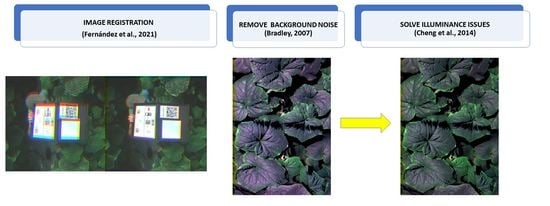
Another problem with these images was the presence of an image background even though removing it is a standard preprocessing technique. As already noted by Wspanialy and Moussa [10], disease detection techniques can be difficult with images having a high degree of background clutter in a greenhouse setting. In our study inside a commercial greenhouse, the first 700 columns of each image were cropped from left to right to remove the white greenhouse aisle. Cropping a section of the image was also used if there were a complex background in a real environment [70]. We also noticed that due to the camera position, only the most exposed leaves were detected, which created dark areas inside the canopy vegetation that also presented some band misalignment. To remove the background cuttler noise as well as some structural wires present in the greenhouse, we created a binary mask using Bradley’s adaptative threshold method [46], which computes a threshold for each pixel using the local mean intensity around the neighborhood of the pixel. This approach is useful due to the internal and external illumination differences among images. It gave better results than the global threshold, which was used in Otsu’s method [71]. The resulting binary mask had a value of 0 for the background area and 1 for the vegetation.

The binary mask overlayed each respective aligned band to obtain band images with their background clutter noise removed and the foreground vegetation retained. The approach we used to remove the background is simpler than the algorithm proposed by Bai et al. [72], which removes non-green background from images acquired over single cucumber leaves that had scabs. Indeed, in their algorithm, a correction method of abnormal points in a 3D histogram of the image was performed followed by rapid segmentation by decreasing histogram dimensions to construct a Gaussian optimization framework to obtain the optimal threshold to isolate the scabs. In addition, Bai et al. [72] worked on images of single cucumber leaves, while in our case we removed the noise from images acquired over the whole plant canopy. Our approach did not need to acquire multiple images as did the method of Wspanialy and Moussa, [10], who studied powdery mildew on greenhouse tomato plants. In this method, which focused on foreground leaves, two images of plants needed to be collected: one was illuminated with a red light to increase the contrast between the foreground leaves and the background. Then the images were converted to grayscale, and Otsu’s method was applied to create a binary mask. The noise was then removed by applying a 3 × 3 median filter to the mask. The filtered mask was then applied to the RGB images. Wspanialy and Moussa’s [10] method was also applied to images acquired at 50 cm from the plant, while in our case the images were collected at 1.5 m above the plant canopy.

One challenge when working with close-range imagery inside a greenhouse is related to the differences in illumination during the image acquisition. Indeed, we observed a bluish-purple coloration over the aligned RGB images due to high illuminance in the blue band. To achieve color consistency, we applied a simple and efficient illumination estimation method developed by Cheng et al. [47]. The method selects bright and dark pixels using a projection distance in the color distribution and then applies a principal component analysis to estimate the illumination direction. Such selection of bright and dark pixels in the image allows obtaining clusters of points with the largest color differences between these pixels.

We trained a fine Gaussian SVM to sort healthy and infected pixels using either individual band reflectance, the RGB composite, several vegetation indices, and all bands together. The overall classification accuracies for the RGB and all the band reflectances together were 93 and 99%, respectively, for the trained model. A major reduction in the overall classification accuracies (57%) was observed when all band reflectances were used. The validation of the SVM model produced the highest overall accuracy with the RGB composite (89%). It was higher than those of Ashhourloo et al. [73], who applied a maximum likelihood classifier to sort healthy wheat leaves and those infected with Puccinia triticina using various vegetation index images derived from hyperspectral data: narrow-band normalized difference vegetation index (83%), NDVI (81%), greenness index (77%), anthocyanin reflectance index (ARI) (75%), structural independent pigment index (73%), physiological reflectance index (71%), plant senescence reflectance index (69%), triangular vegetation index (69%), modified simple ratio (68%), normalized pigment chlorophyll ratio index (68%), and nitrogen reflectance index (67%). Our accuracy was also higher than those reported by Pineda et al. [34], who tested an artificial neural network (70%), a logistic regression analysis (73%), and an SVM (46%) to classify multicolor fluorescence images acquired over healthy and infected zucchini leaves with powdery mildew.

However, our accuracies with both the training and validating datasets were lower than in Berdugo et al. [33] (overall accuracy of 100%), who applied a stepwise discriminant analysis to discriminate healthy cucumber leaves from those infected with powdery mildew using the following features: effective quantum yield, SPAD 502 Plus Chlorophyll Meter (Spectrum Technologies, Inc., Aurora, IL, USA) values, maximum temperature difference (MTD), NDVI and ARI. Our overall classification accuracies were also lower than those reported by Thomas et al. [69] (94%), who applied a non-linear SVM over a combination of pseudo-RGB representation and spectral information from hyperspectral images to classify powdery mildew caused by Blumeria graminis f. sp. Hordei in barley. Our overall classification accuracies were also lower than those of Kong et al. [18], who applied a partial least square discriminant analysis (PLS–DA) (94%), a radial basis function neural network (RBFNN) (98%), an extreme learning machine (ELM) (99%), and a support vector machine (SVM) (99%) to hyperspectral images for classifying healthy pixels and those infected with Sclerotinia sclerotiorum on oilseed rape plants

5. Conclusions

Our study tested the use of ungeoreferenced close-range multispectral Micasense RedEdge images to detect powdery mildew over greenhouse cucumber plants. The images were spatially and spectrally corrected and used to compute vegetation index images. The resulting images were entered in an SVM classifier to sort pixels as a function of their status (healthy and infected). The best overall accuracy obtained with the validation dataset was achieved with the RGB composite (89%) and with the PMVI-2 image (81.83%). The present work is part of an ongoing research project to build an automatic cucumber powdery mildew detection system for commercial greenhouses. While presenting preliminary results, we introduced for the first time close-range multispectral imagery for detecting cucumber powdery mildew under real commercial conditions. The proposed methodology is based on proved methods for image registration and band alignment of close-distance imagery collected at the canopy level. At the same time, we achieved color constancy over each image by using the illumination correction method of Cheng et al. [47] and calibrated an SVM classifier to sort healthy and infected pixels.

However, further work is needed to test the classifier over a large dataset that will allow the use of other classifiers such as ANN or Deep Learning algorithms. There is also the need to determine the best distance to collect the image of the individual leaves. The images were acquired with a camera mounted on a cart and it is necessary to analyze the effect of potential cart vibrations on the image quality. The analysis used commercial software (MATLAB) and there is the need to adapt the method to open-source software. Our study was able to detect infected pixels in MicaSense RedEdge imagery but only when the symptoms were visible. Further work is needed to test the imagery before the symptoms become apparent. Fernández et al. [20] already showed that leaves infected by powdery mildew can be detected 48 h before symptoms become apparent using the scores of the first two principal components computed by a principal component analysis applied to reflectance spectra between 400 to 900 nm.

References

1. Agriculture and Agri-Food Canada. 2020. Available online: https://www.agr.gc.ca/eng/canadas-agriculture-sectors/horticulture/horticulture-sector-reports/statistical-overview-of-the-canadian-greenhouse-vegetable-industry-2019/?id=1609252451699 (accessed on 6 June 2021).
2. Khater, M.; de la Escosura-Muñiz, A.; Merkoçi, A. Biosensors for plant pathogen detection. Biosens. Bioelectron. 2017, 93, 72–86. [Google Scholar] [CrossRef] [Green Version]
3. Hafez, Y.M.; Attia, K.A.; Kamel, S.; Alamery, S.F.; El-Gendy, S.; Al-Doss, A.A.; Mehiar, F.; Ghazy, A.I.; Ibrahim, E.I.; Abdelaal, K.A.A. Bacillus subtilis as a bio-agent combined with nano molecules can control powdery mildew disease through histochemical and physiobiochemical changes in cucumber plants. Physiol. Mol. Plant Pathol. 2020, 111, 101489. [Google Scholar] [CrossRef]
4. Spanu, P.D.; Panstruga, R. Biotrophic Plant-Microbe Interactions. Front. Plant Sci. 2017, 8, 192. [Google Scholar] [CrossRef] [PubMed] [Green Version]
5. Li, M.; Zhao, C.; Li, D.; Yang, X.; Sun, C.; Wang, Y. Towards developing an early warning system for cucumber diseases for greenhouse in China. In Proceedings of the 1st IFIP TC 12 International Conference on Computer and Computing Technologies in Agriculture (CCTA 2007), Wuyishan, China, 18–20 August 2007; pp. 1375–1378. [Google Scholar]
6. Wang, H.; Li, M.L.; Xu, J.P.; Chen, M.X.; Li, W.Y.; Li, M. An early warning method of cucumber downy mildew in solar greenhouse based on canopy temperature and humidity modeling. Ying Yong Sheng Tai Xue Bao 2015, 26, 3027–3034. [Google Scholar]
7. Yang, X.; Li, M.; Zhao, C.; Zhang, Z.; Hou, Y. Early warning model for cucumber downy mildew in unheated greenhouses. N. Z. J. Agric. Res. 2007, 50, 1261–1268. [Google Scholar] [CrossRef]
8. Bock, C.H.; Parker, P.E.; Cook, A.Z.; Gottwald, T.R. Visual rating and the use of image analysis for assessing different symptoms of citrus canker on grapefruit leaves. Plant Dis. 2008, 92, 530–541. [Google Scholar] [CrossRef] [Green Version]
9. Bock, C.H.; Cook, A.Z.; Parker, P.E.; Gottwald, T.R. Automated image analysis of the severity of foliar citrus canker symptoms. Plant Dis. 2009, 93, 660–665. [Google Scholar] [CrossRef] [PubMed]
10. Wspanialy, P.; Moussa, M. Early powdery mildew detection system for application in greenhouse automation. Comp. Electron. Agric. 2016, 127, 487–494. [Google Scholar] [CrossRef]
11. Zhang, S.; Wu, X.; You, Z.; Zhang, L. Leaf image-based cucumber disease recognition using sparse representation classification. Comp. Electron. Agric. 2017, 134, 135–141. [Google Scholar] [CrossRef]
12. Zhang, S.; Zhang, S.; Zhang, C.; Wang, X.; Shi, Y. Cucumber leaf disease identification with global pooling dilated convolutional neural network. Comp. Electron. Agric. 2019, 162, 422–430. [Google Scholar] [CrossRef]
13. Es-Saady, Y.; El Massi, Y.; Mammass, D.; Benazoun, A. Automatic recognition of plant leaves diseases based on a serial combination of two SVM classifiers. In Proceedings of the International Conference on Electrical and Information Technologies (ICEIT), Tangiers, Morocco, 4–7 May 2016; pp. 561–566. [Google Scholar] [CrossRef]
14. Islam, M.; Dinh, A.; Bhowmik, P. Detection of potato diseases using image segmentation and multiclass support vector machine. In Proceedings of the IEEE 30th Canadian Conference on Electrical and Computer Engineering (CCEC), Windsor, ON, Canada, 30 April–3 May 2017; pp. 1–4. [Google Scholar] [CrossRef] [Green Version]
15. Shi, Y.; Huang, W.; Ye, H.; Ruan, C.; Xing, N.; Geng, Y.; Dong, Y.; Peng, D. Partial least square discriminant analysis based on normalized two-stage vegetation indices for mapping damage from rice diseases using PlanetScope datasets. Sensors 2018, 18, 1901. [Google Scholar] [CrossRef] [Green Version]
16. Mahlein, A.-K.; Steiner, U.; Hillnhütter, C.; Dehne, H.W.; Oerke, E.C. Hyperspectral imaging for small-scale analysis of symptoms caused by different sugar beet diseases. Plant Methods 2012, 8, 3. [Google Scholar] [CrossRef] [PubMed] [Green Version]
17. Folch-Fortuny, A.; Prats-Montalban, J.M.; Cubero, S.; Blasco, J.; Ferrer, A. VIS/NIR hyperspectral imaging and N-way PLS-DA models for detection of decay lesions in citrus fruits. Chemom. Intell. Lab. Syst. 2016, 156, 241–248. [Google Scholar] [CrossRef] [Green Version]
18. Kong, W.; Zhang, C.; Huang, W.; Liu, F.; He, Y. Application of hyperspectral imaging to detect Sclerotinia sclerotiorum on Oilseed rape stems. Sensors 2018, 18, 123. [Google Scholar] [CrossRef] [Green Version]
19. Atanassova, S.; Nikolov, P.; Valchev, N.; Masheva, S.; Yorgov, D. Early detection of powdery mildew (Podosphaera xanthii) on cucumber leaves based on visible and near-infrared spectroscopy. In Proceedings of the 10th Jubilee International Conference of the Balkan Physical Union, Sofia, Bulgaria, 26–30 August 2019; Volume 2075, p. 160014. [Google Scholar] [CrossRef]
20. Fernández, C.I.; Leblon, B.; Haddadi, A.; Wang, K.; Wang, J. Detecting Cucumber Powdery Mildew with Hyperspectral Data. Can. J. Plant Sci. 2021, submitted. [Google Scholar]
21. Zhang, M.; Liu, X.; O’Neill, M. Spectral discrimination of Phytophthora infestans infection on tomatoes based on principal component and cluster analyses. Int. J. Remote Sens. 2002, 23, 1095–1107. [Google Scholar] [CrossRef]
22. Dutta, S.; Singh, S.K.; Panigrahy, S. Assessment of late blight induced potato crops: A case study for West Bengal District using temporal AWiFS and MODIS data. J. Indian Soc. Remote Sens. 2014, 42, 353–361. [Google Scholar] [CrossRef]
23. Fernández, C.I.; Leblon, B.; Haddadi, A.; Wang, J.; Wang, K. Potato late blight detection at the leaf and canopy level using hyperspectral data. Can. J. Remote Sens. 2020, 46, 390–413. [Google Scholar] [CrossRef]
24. Zhang, M.; Qin, Z.; Liu, X.; Ustin, S.L. Detection of stress in tomatoes induced by late blight disease in California, USA, using hyperspectral remote sensing. Int. J. Appl. Earth Obs. Geoinf. 2003, 4, 295–310. [Google Scholar] [CrossRef]
25. Ray, S.S.; Jain, N.; Arora, R.K.; Chavan, S.; Panigrahy, S. Utility of hyperspectral data for potato late blight disease detection. J. Indian Soc. Remote Sens. 2011, 39, 161–169. [Google Scholar] [CrossRef]
26. Franceschini, M.H.D.; Bartholomeus, H.; Van Apeldoorn, D.; Suomalainen, J.; Kooistra, L. Feasibility of unmanned aerial vehicle optical imagery for early detection and severity assessment of late blight in potato. Remote Sens. 2019, 11, 224. [Google Scholar] [CrossRef] [Green Version]
27. Fernández, C.I.; Leblon, B.; Haddadi, A.; Wang, K.; Wang, J. Potato late blight detection at the leaf and canopy levels based in the red and red-edge spectral regions. Remote Sens. 2020, 12, 1292. [Google Scholar] [CrossRef] [Green Version]
28. Bodria, L.; Fiala, M.; Oberti, R.; Naldi, E. Chlorophyll fluorescence sensing for early detection of crop diseases symptoms. In Proceedings of the 2002 American Society of Agricultural and Biological Engineers (ASABE) Annual Meeting, Chicago, IL, USA, 28–31 July 2002; pp. 1–15. [Google Scholar] [CrossRef]
29. Leufen, G.; Noga, G.; Hunsche, M. Proximal sensing of plant-pathogen interactions in spring barley with three fluorescence techniques. Sensors 2014, 14, 11135–11152. [Google Scholar] [CrossRef] [Green Version]
30. Mahlein, A.-K. Plant disease detection by imaging sensors—parallels and specific demands for precision agriculture and plant phenotyping. Plant Dis. 2015, 100, 241–251. [Google Scholar] [CrossRef] [Green Version]
31. Belasque, J.; Gasparoto, M.C.G.; Marcassa, L.G. Detection of mechanical and disease stresses in citrus plants by fluorescence spectroscopy. Appl. Opt. 2008, 47, 1922–1926. [Google Scholar] [CrossRef] [PubMed]
32. Buschmann, C.; Lichtenthaler, H.K. Principles and characteristics of multi-colour fluorescence imaging of plants. J. Plant Physiol. 1998, 152, 297–314. [Google Scholar] [CrossRef]
33. Berdugo, C.A.; Zito, R.; Paulus, S.; Mahlein, A.-K. Fusion of sensor data for the detection and differentiation of plant diseases in cucumber. Plant Pathol. 2014, 63, 1344–1356. [Google Scholar] [CrossRef]
34. Pineda, M.; Luisa Perez-Bueno, M.; Paredes, V.; Barón, M. Use of multicolor fluorescence imaging for the diagnosis of bacterial and fungal infection on zucchini by implementing machine learning. Funct. Plant Biol. 2017, 44, 563–572. [Google Scholar] [CrossRef] [Green Version]
35. Polonio, Á.; Pineda, M.; Bautista, R.; Martínez-Cruz, J.; Pérez-Bueno, M.L.; Barón, M.; Pérez-García, A. RNA-seq analysis and fluorescence imaging of melon powdery mildew disease reveal an orchestrated reprogramming of host physiology. Sci. Rep. 2019, 9, 7978. [Google Scholar] [CrossRef] [Green Version]
36. Kuckenberg, J.; Tartachnyk, I.; Noga, G. Temporal and spatial changes of chlorophyll fluorescence as a basis for early and precise detection of leaf rust and powdery mildew infections in wheat leaves. Precis. Agric. 2009, 10, 34–44. [Google Scholar] [CrossRef]
37. Sandmann, M.; Grosh, R.; Graefe, J. The use of features from fluorescence, thermography, and NDVI imaging to detect biotic stress in lettuce. Plant Dis. 2018, 102, rs6065107. [Google Scholar] [CrossRef] [PubMed] [Green Version]
38. Wang, S.; Yang, D.M.; Rong, R.; Zhan, X.; Xiao, G. Pathology image analysis using segmentation deep learning algorithms. Am. J. Pathol. 2019, 189, 1686–1698. [Google Scholar] [CrossRef] [Green Version]
39. Anderson, R.; Bayer, P.; Edwards, D. Climate change and the need for agricultural adaptation. Curr. Opin. Plant Biol. 2020, 56, 197–202. [Google Scholar] [CrossRef]
40. Fernández, C.I.; Leblon, B.; Haddadi, A.; Wang, K.; Wang, J. Comparison between three registration methods in the case of non-georeferenced close range of multispectral images. Remote Sens. 2021, 13, 396. [Google Scholar] [CrossRef]
41. Medina, G.; (Micasense, Inc., Seattle, Washington, DC, USA). Personal communication, 2021.
42. Eskandari, S.; Sharifnabi, B. The modifications of cell wall composition and water status of cucumber leaves induced by powdery mildew and manganese nutrition. Plant Physiol. Biochem. 2019, 145, 132–141. [Google Scholar] [CrossRef]
43. Atole, R.R.; Park, D. A multiclass deep convolutional neural network classifier for detection of common rice plants anomalies. Int. J. Adv. Comput. Sci. Appl. 2018, 9, 67–70. [Google Scholar]
44. Ozguven, M.M.; Adem, K. Automatic detection and classification of leaf spot disease in sugar beet using deep learning algorithms. Phys. A 2019, 122537. [Google Scholar] [CrossRef]
45. Kociolek, M.; Strzelecki, M.; Obuchowicz, R. Does image normalization and intensity resolution impact texture classification? Comput. Med. Imaging Graph. 2020, 101716. [Google Scholar] [CrossRef]
46. Bradley, D.; Roth, G. Adapting thresholding using the integral image. J. Graph. Tools 2007, 12, 13–21. [Google Scholar] [CrossRef]
47. Cheng, D.; Prasad, D.K.; Brown, M.S. Illuminant estimation for color constancy: Why spatial-domain methods work and the role of the color distribution. J. Opt. Soc. Am. 2014, 31, 1049–1058. [Google Scholar] [CrossRef]
48. Jordan, C.F. Derivation of leaf area index from quality of light on the forest floor. Ecology 1969, 50, 663–666. [Google Scholar] [CrossRef]
49. Rouse, J.W.; Haas, R.; Schell, J.; Deering, D. Monitoring vegetation systems in the Great Plains with ERTS. In Proceedings Third Earth Resources Technology Satellite-1 Symposium; Paper A-20; National Aeronautics and Space Administration (NASA), NASA, Goddard Space Flight Center: Washington, DC, USA, 1974; Volume 1, pp. 309–317. Available online: https://ntrs.nasa.gov/api/citations/19740022614/downloads/19740022614.pdf (accessed on 6 June 2021).
50. Tucker, C.J. Red and photographic infrared linear combinations for monitoring vegetation. Remote Sens. Environ. 1979, 8, 127–150. [Google Scholar] [CrossRef] [Green Version]
51. Matsushita, B.; Taung, W.; Chen, J.; Onda, Y.; Qiu, G. Sensitivity of the enhanced vegetation index (EVI) and normalized difference vegetation index (NDVI) to topographic effects: A case study in high-density Cypress forest. Sensors 2007, 7, 2636–2651. [Google Scholar] [CrossRef] [Green Version]
52. Huete, A.R. A soil-adjusted vegetation index (SAVI). Remote Sens. Environ. 1988, 25, 295–309. [Google Scholar] [CrossRef]
53. Rondeaux, G.; Steven, M.; Baret, F. Optimization of soil-adjusted vegetation indices. Remote Sens. Environ. 1996, 55, 95–107. [Google Scholar] [CrossRef]
54. Zhu, L.; Zhao, X.; Jai, L.; Wang, J.; Jiang, L.; Ding, J.; Liu, N.; Yu, Y.; Li, J.; Xiao, N.; et al. Soil TPH concentration estimation using vegetation indices in an oil-polluted area of Eastern China. PLoS ONE. 2013, 8, e54028. [Google Scholar] [CrossRef] [Green Version]
55. Gitelson, A.A.; Viña, A.; Ciganda, V.; Rundquist, D.C.; Arkebauer, T.J. Remote estimation of canopy chlorophyll content in crops. Geophys. Res. Lett. 2005, 32, 20–26. [Google Scholar] [CrossRef] [Green Version]
56. Mirik, M.; Ansley, R.J.; Michels Jr, J.; Elliot, N.C. Spectral vegetation indices selected for quantifying Russian wheat aphid (Diuraphs noxia) feeding damage in wheat (Triticum aestivum L.). Precis. Agric. 2012, 13, 501–516. [Google Scholar] [CrossRef]
57. Escadafal, R.; Huete, A. Etude des propriétés spectrales des sols arides appliquée à l’amélioration des indices de végétation obtenus par télédétection. Comptes Rendus L’Académie Sci. 1991, 132, 1385–1391. [Google Scholar]
58. Gitelson, A.A.; Merzlyak, M.N.; Lichtenthaler, H.K. Detection of red-edge position and chlorophyll content by reflectance measurements near 700 nm. J. Plant Physiol. 1996, 148, 501–508. [Google Scholar] [CrossRef]
59. Sharma, L.K.; Bu, H.; Denton, A.; Franzen, D.W. Active-Optical sensors using red NDVI compared to red-edge NDVI for prediction of corn grain yield in North Dakota, U.S.A. Sensors 2015, 15, 27832–27853. [Google Scholar] [CrossRef] [PubMed]
60. Haddadi, A.; Leblon, B. Developing a UAV-Based Camera for Precision Agriculture; Final Report. Mitacs # IT07423 Grant; University of New Brunswick, Faculty of Forestry and Environmental Management: Fredericton, NB, Canada, 2018; 106p. [Google Scholar]
61. Mantero, P.; Moser, G.; Serpico, S.B. Partially supervised classification of remote sensing images through SVM-based probability density estimation. IEEE Trans. Geosci. Remote Sens. 2005, 43, 559–570. [Google Scholar] [CrossRef]
62. Raghavendra, S.; Deka, P.C. Support vector machine applications in the field of hydrology: A review. Appl. Soft Comp. 2014, 19, 372–386. [Google Scholar] [CrossRef]
63. Olson, M.; Wyner, J.A.; Berk, R. Modern neural networks generalize on small data sets. In Proceedings of the 32nd Conference on Neural Information Processing Systems (NeurIPS, 2018), Montreal, QC, Canada, 3–8 December 2018; pp. 3619–3628. [Google Scholar]
64. Paoletti, M.E.; Haut, J.M.; Plaza, J.; Plaza, A. Deep learning classifiers for hyperspectral imaging: A review. ISPRS J. Photogramm. Remote Sens. 2019, 158, 279–317. [Google Scholar] [CrossRef]
65. Zhang, J.; Huang, Y.; Pu, R.; Gonzalez-Moreno, P.; Yuan, L.; Wu, K.; Huang, W. Monitoring plant diseases and pests through remote sensing technology: A review. Comput. Electron. Agric. 2019, 165, 104943. [Google Scholar] [CrossRef]
66. Ferentinos, K.P. Deep learning models for plant disease detection and diagnosis. Comput. Electron. Agric. 2018, 145, 311–318. [Google Scholar] [CrossRef]
67. Fahrentrapp, J.; Ria, F.; Geilhausen, M.; Panassiti, B. Detection of gray mold leaf infections prior to visual symptom appearance using a five-band multispectral sensor. Front. Plant Sci. 2019, 10, 628. [Google Scholar] [CrossRef] [Green Version]
68. Kuppala, K.; Banda, S.; Barige, T.R. An overview of deep learning methods for image registration with focus on feature-based approaches. Int. J. Image Data Fusion 2020, 11, 113–135. [Google Scholar] [CrossRef]
69. Thomas, S.; Behmann, J.; Steier, A.; Kraska, T.; Muller, O.; Rascher, U.; Mahlein, A.-K. Quantitative assessment of disease severity and rating of barley cultivars based on hyperspectral imaging in a non-invasive, automated phenotyping platform. Plants Methods 2018, 14–45. [Google Scholar] [CrossRef] [Green Version]
70. Vishnoi, V.K.; Kumar, K.; Kumar, B. Plant disease detection using computational intelligence and image processing. J. Plant Dis. Prot. 2020, 128, 19–53. [Google Scholar] [CrossRef]
71. Otsu, N. A threshold selection method from gray-level histograms. IEEE Trans. Syst. Man Cyber. 1979, 9, 62–66. [Google Scholar] [CrossRef] [Green Version]
72. Bai, X.; Fu, Z.; Stankovski, S.; Wang, X.; Li, X. A three-dimensional threshold algorithm based on histogram reconstruction and dimensionality reduction for registering cucumber powdery mildew. Comput. Electron. Agric. 2019, 158, 211–218. [Google Scholar] [CrossRef]
73. Ashhourloo, D.; Mobasheri, M.R.; Huete, A. Evaluating the effect of different wheat rust disease symptoms on vegetation indices using hyperspectral measurements. Remote Sens. 2014, 6, 5107–5123. [Google Scholar] [CrossRef] [Green Version]
Figure 1. Rows of cucumber plants in the greenhouse.
Remotesensing 13 02948 g001
Figure 2. (a) Micasense® RedEdge camera and related distance between the five sensors (adapted from www.dronenerds.com (accessed on 10 December 2020)); (b) Designed cart for image acquisition.
Remotesensing 13 02948 g002
Figure 3. RGB composite made with the Micasense® RedEdge multispectral images acquired over the MicaSense® calibration panel.
Remotesensing 13 02948 g003
Figure 4. Flowchart of the image processing used in the study.
Remotesensing 13 02948 g004
Figure 5. Comparison between (a) aligned and masked RGB cucumber canopy images and (b) the same image after applying the illumination correction.
Remotesensing 13 02948 g005
Figure 6. Comparisons between an aligned RGB close-range image and related vegetation index images from Table 2. (a) RGB composite; (b) Simple Ratio; (c) Normalized Difference Vegetation Index; (d) Difference Vegetation Index; (e) Enhanced Vegetation Index; (f) Soil-Adjusted Vegetation Index (L is equal to 0.5); (g) Optimized Soil-Adjusted Vegetation Index; (h) Optimized Soil-Adjusted Vegetation Index 2; (i) Green Chlorophyll Index; (j) Green Normalized Difference Vegetation Index; (k) Redness Index; (l) Red-Edge Chlorophyll Index; (m) Red-Edge Normalized Difference Vegetation Index; (n) Powdery Mildew Vegetation Index; (o) Powdery Mildew Vegetation Index 2.
Remotesensing 13 02948 g006
Figure 7. Boxplots comparing the reflectance of healthy and infected pixels from each multispectral band for the whole data set (n = 1000) used to train and validate the Support Vector Machine.
Remotesensing 13 02948 g007