Article

The Impact of Phenological Developments on Interferometric and Polarimetric Crop Signatures Derived from Sentinel-1: Examples from the DEMMIN Study Site (Germany)

1
Department of Geoecology, Institute of Geosciences and Geography, University of Halle-Wittenberg, 06120 Halle (Saale), Germany
2
Department of Remote Sensing, Institute of Geography and Geology, University of Würzburg, 97074 Würzburg, Germany
3
Department of Physical Geography, Institute of Geography and Geology, University of Würzburg, 97074 Würzburg, Germany
*
Author to whom correspondence should be addressed.
Remote Sens. 2021, 13(15), 2951; https://doi.org/10.3390/rs13152951
Submission received: 11 June 2021 / Revised: 22 July 2021 / Accepted: 23 July 2021 / Published: 27 July 2021

Abstract

:
This study explores the potential of Sentinel-1 Synthetic Aperture Radar (SAR) to identify phenological phases of wheat, sugar beet, and canola. Breakpoint and extreme value analyses were applied to a dense time series of interferometric (InSAR) and polarimetric (PolSAR) features recorded during the growing season of 2017 at the JECAM site DEMMIN (Germany). The analyses of breakpoints and extrema allowed for the distinction of vegetative and reproductive stages for wheat and canola. Certain phenological stages, measured in situ using the BBCH-scale, such as leaf development and rosette growth of sugar beet or stem elongation and ripening of wheat, were detectable by a combination of InSAR coherence, polarimetric Alpha and Entropy, and backscatter (VV/VH). Except for some fringe cases, the temporal difference between in situ observations and breakpoints or extrema ranged from zero to five days. Backscatter produced the signature that generated the most breakpoints and extrema. However, certain micro stadia, such as leaf development of BBCH 10 of sugar beet or flowering BBCH 69 of wheat, were only identifiable by the InSAR coherence and Alpha. Hence, it is concluded that combining PolSAR and InSAR features increases the number of detectable phenological events in the phenological cycles of crops.

1. Introduction

Phenology is defined by the International Biological Program as, “study of the timing of recurrent biological events, the causes of their timing with regard to biotic and abiotic factors, and the interrelation among phases of the same or different species” [1]. As such, phenology can provide information about a plant’s health, growth, and productivity, for example, regarding biomass. This kind of information is crucial for crop management [2,3] and crop yield prediction because plant productivity and growth are more sensitive to meteorological conditions in particular phenological stages [4]. In the context of this study, macro stadia also are referenced as phenological stages or phases, whereas a micro stadium is referred to as a phenological event. Remote sensing and especially active microwave remote sensing provide established tools for providing such information at various spatial and temporal resolutions [5]. The interaction of the radar signal with vegetation has been widely investigated for roughly four decades. During field campaigns, it was discovered that radar backscatter is sensitive to vegetation cover and soil moisture [6,7]. The launch of RADARSAT-1 and ERS-1 during the 1990s as well as later launches of RADARSAT-2, TerraSAR-X, and TanDEM-X further pushed the advances made in the field of radar-based environmental monitoring [5,8,9], including applications in agriculture. In 1995 the usage repeat pass interferometry exhibited low coherence values for densely vegetated fields and high coherence values for bare and stubbled fields, allowing for the detection of farming activities [10]. During the following decade, it was demonstrated that Synthetic Aperture Radar (SAR) sensors can derive crop height of sugarcane and monitor its harvesting period [11]. The same study showed X-band outperforming L-and C-band sensors at the distinction of bare and vegetated soil, increased sensitivity of cross-polarisation towards harvesting events, and high correlation between time series of Normalized Difference Vegetation Index (NDVI) and SAR backscatter. As for crop phenology, the derivation of three different phenological intervals was achieved by employing polarimetric entropy or co-polarised interferometric coherence in combination with cross-polarised intensity computed from quad-polarimetric RADARSAT-2 data [12]. Polarimetric features [13] derived from the same satellite were utilised to develop a tracking framework for crop phenology of spring wheat and canola that showed a strong correlation (R2 0.66–0.91) between Alpha angle and plant height, which could be further increased (R2 0.88–0.98) by applying temporal smoothing [14].
The launch of Sentinel-1 (S-1) A and B addressed one major issue of the above-mentioned studies: data availability. For Europe, this new C-Band SAR data is available every six days [15,16,17]. This increased availability of open SAR data facilitated research of dense time series at a spatial resolution of 10 m to 20 m. In addition, effects of climate change, such as increasing severity of extreme weather events, have fostered the attentiveness towards SAR-based phenology monitoring [5,16,18]. Hence, several studies demonstrated the validity of using dense SAR time series to monitor the phenological development of crops [16,19,20,21,22]. Combined with advances in the field of cloud computing, derivation of the start, peak, and end of the season were conducted across Europe [23]. However, the above-named studies focus either on a single crop type [19,20,21], a specific phenological event such as the flowering of canola [21], a rather coarse distinction of phenological events, for example, date of emergence and harvest or start and end of the season [22,23], mainly rely on training/validation data not georeferenced to a specific field [16,23], or have a limited set of SAR features, for example, just backscatter [23]. Furthermore, the issue has been raised by Meroni et al. (2021) [23] and Shang et al. (2020) [24] that georeferenced field measurements are necessary to truly understand the potential of phenology estimations based on dense SAR time series.
To address this research gap, this study combines a comparatively large set of S-1-features: polarimetric Alpha and Entropy [13], VV and VH InSAR coherence, Kennaugh Matrix Elements (K0, K1, K5, K6) [25], and backscatter (VV and VH), with georeferenced field observations to track phenological development of three crop types: wheat, sugar beet, and canola, across the growing season of 2017 by applying breakpoint and extreme value analyses, which have been successfully employed in related studies [16,21,26,27]. Besides the detection of macro stadia, such as flowering, or micro stadia, such as soft dough [28], this study addresses the transition from vegetative to reproductive period. The latter is of particular interest because a balanced ratio between those two periods is crucial for the overall plant productivity and the transition itself is considered the most dramatic change of plant development [29,30]. Therefore, this transition period marks a time of increased vulnerability of the plant, which is of special interest in crop and risk management [23,31]. The objectives of this study are described as following: (i) assess the complementary value of polarimetric and interferometric S-1-features for monitoring crop phenology, (ii) identify phenological events or stages on crop signatures, and (iii) detect the transition from vegetative to reproductive stage.

2. Materials and Methods

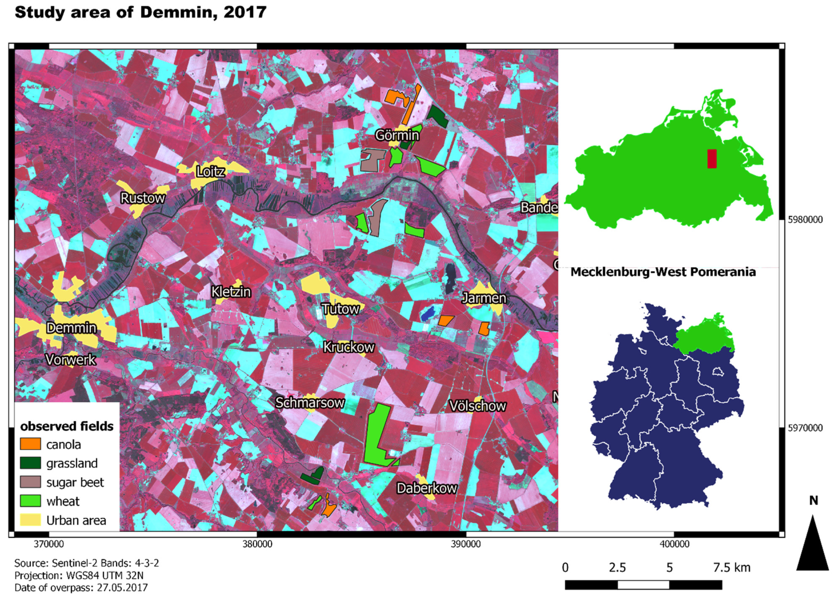
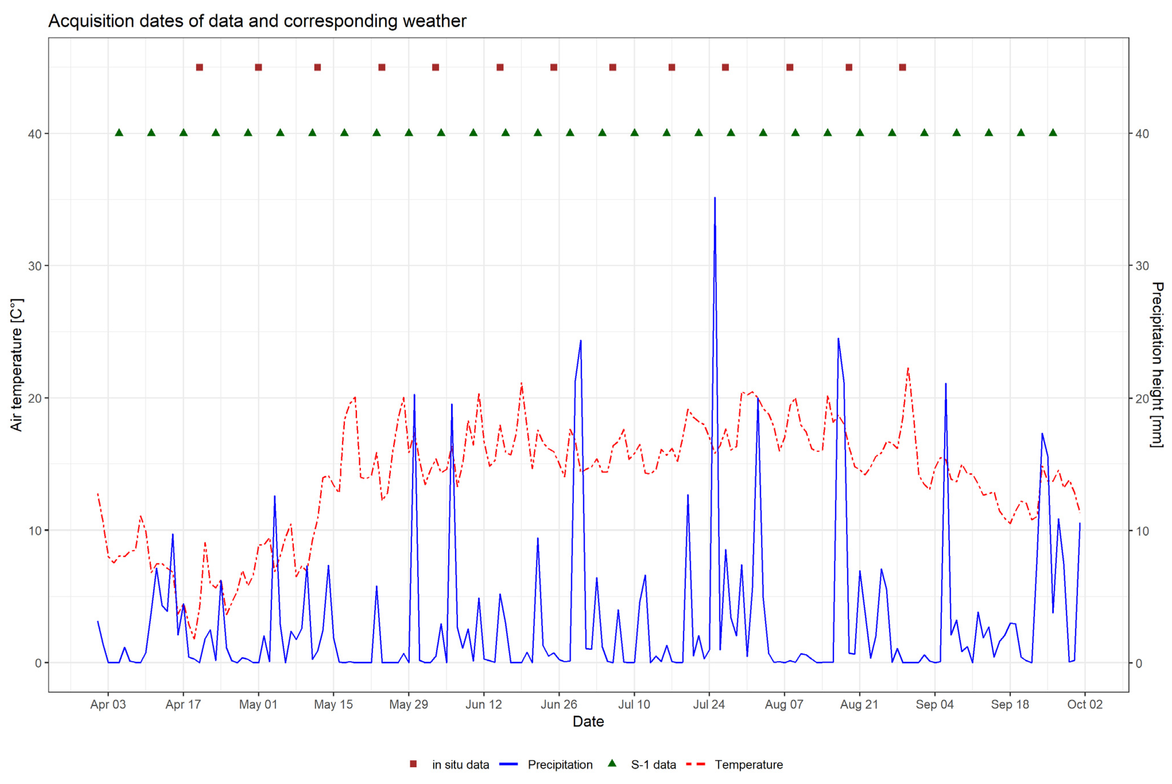
2.1. Study Area and In Situ Data

The study was conducted in Mecklenburg-West Pomerania, the north-eastern federal state of Germany. The climate of the study area is characterised by a mean air temperature of 8.3 °C and an average sum of precipitation of around 550 mm. Therefore, it is classified as temperate Middle-European, including perennial humidity [32].
From 2001 onwards, the test site, the Durable Environmental Multidisciplinary Monitoring Information Network (DEMMIN), has been an established calibration and validation site for earth observation missions by the German Aerospace Center (DLR). Since 2008, DEMMIN is commonly operated by DLR and the Geo-Research-Centre Potsdam (GFZ) as a Terrestrial Environmental Observatoria (TERENO) site, and in 2018 it became an official member of the Joint Experiment for Crop Assessment and Monitoring (JECAM) [33].
The in situ collected data on crop phenology were provided by the GFZ as part of the DEMMIN monitoring framework (see below) for the growing season of 2017. The data were recorded from 20 April to 29 August 2017 every ten to twelve days. In total, the ground truth data encompasses 13 timesteps. The locations of the measurements cover one to two measuring points for eight fields of wheat, five fields of canola, two fields of sugar beet, and four patches of grassland (Figure 1). In this study, grassland is used as a reference for natural vegetation (see Section 2.3.1 for further information). Every time step consists of measurements regarding plant height and row distance in centimetres, crop cover in percentage, the number of leaves, as well as the phenology code. The latter was estimated based on the BBCH-scale. BBCH is an acronym for Biologische Bundesanstalt für Forst und Landwirtschaft, Bundessortenamt für CHemische Industrie [28]. As most of the measuring points were close to roads or field tracks, polygons were drawn for the respective fields linked to the in situ measurement to avoid the influence of mixed pixels.
Additionally, phenological data provided by the German Weather Service (DWD) was acquired to cross-reference the observations of the GFZ, fill in data gaps for canola fields, and better understand fringe cases of the time series. This DWD data (Table 1) contains observation dates of important phenological events. For canola, the end of flowering, harvest, germination, bud development, and the preparation of the field are observed. The data was retrieved for the three nearest observation posts (distances to the study area ranging from 15 km to 25 km) and only for canola and wheat, as sugar beet was sufficiently covered by the GFZ data.
Figure 2 depicts the development of temperature and precipitation in DEMMIN during the observation period in 2017. It also indicates the acquisition dates for both field data and SAR acquisitions, which are presented in the following section.

2.2. Sentinel-1 Time Series

The time series of S-1 A and B was available from 5 April to 26 September 2017 at six-day intervals encompassing 30 scenes. The data was acquired in Interferometric Wide Swath Mode and VV/VH dual-polarisation. Single Look Complex (SLC) was selected [34] to process polarimetric features and interferometric coherences. The pre-processing was accomplished by using the software packages IDL (version 8), ENVI (version 5), and SNAP (version 7). Hereby, ENVI/IDL was used for data management purposes and SNAP for the actual processing of the SLC files. This framework followed the steps provided by the literature [35,36]. The processing of the polarimetric features included terrain flattening [37], multi-looking with one look in azimuth and three looks in range, speckle filtering by a 5 pixel × 5 pixel boxcar filter, and Range-Doppler Terrain-Correction [38] resulting in gamma nought (GN) intensities of 20 m × 20 m pixel size. The interferometric (InSAR) coherence is computed after removing flat earth and topographic phase using a moving window of three pixels in azimuth and eleven pixels in range, while the subsequent parameters for multi-looking and terrain correction remain unchanged. The SRTM data (1-Arc-Second) served as a digital elevation model in the processing. InSAR coherences were computed using a 6-day temporal baseline and consecutive master images [39].
Table 2 lists the computed S-1 features alongside their abbreviations, units, and the information provided by them. This list contains VV and VH InSAR coherence as a measurement of temporal decorrelation [40,41,42], which may reflect major changes in plant physiognomy, as demonstrated by Schlund and Erasmi (2020) [16]. Additionally, Entropy and Alpha are calculated from the Covariance-matrix (C2) [13], providing information about the depolarisation [43,44]. However, for the VV/VH-polarised data, Alpha represents the relation between both polarisations, as the phase relation between VV and HH is unknown [35]. The validity of polarimetric decomposition for estimating plant phenology as well as biophysical parameters has been shown by various studies [12,14,45,46]. Finally, the Kennaugh Matrix elements [25] were included in the analyses. K0 and K1 are intensity-only features, which represent the combined backscatter (K0) (span) and the difference between complex signals of VH and VV (K1). K5 and K6 contain the real and imaginary parts of the inter-channel correlation. These two features exhibit high sensitivity to deterministic, mostly artificially-created, targets [25].

2.3. Methods

2.3.1. Elementary Analysis of S-1 Features

This analysis assesses the inherent variance of the time series for each crop type by using descriptive statistics. For this, the class of grassland is included because it provides a reference to more heterogeneous vegetation than a single crop type. If an S-1 feature displays a similar behaviour for a crop type compared to grassland, it is assumed that this feature is overly sensitive to environmental influences, such as wind or precipitation, and, therefore, cannot reflect the general trends induced by phenological development. For this purpose, pixel-based statistical parameters (mean, standard deviation, minimum, maximum, 25%-, 50%-, and 75%-quartiles) are computed for each crop type and grassland, using the entire time series. These statistics are then displayed as box and scatter plots per crop type. An S-1 feature is assessed unsuitable for crop phenology monitoring if crops exhibit interquartile ranges (IQR; distance between the 25%- and 75%-quartiles) and median values like grassland. Furthermore, standard deviations are seen as indicators of a stronger signal response towards phenological development. In addition, a correlation analysis encompassing all S-1 features and the recorded plant parameters was conducted to reveal statistical redundancies and dependencies between features and biophysical parameters. Plant height and crop cover are included in this analysis because they are crucial parameters for describing phenological development [14,28]. These inclusions serve as an additional verification of the assumption that S-1 signatures reflect plant development as described by the BBCH-scale. Therefore, a fixed number of pixels is extracted from each field to avoid weighting by field size; the number is chosen based on the size of the smallest field.

2.3.2. Signature Analysis

Individual crop signatures were created by smoothing raw time series data to reduce the impact of outliers and to enable the extraction of general patterns for each SAR feature and crop type. For this purpose, locally weighted scatterplot smoothing (LOESS) [47] with a linear regression model was employed. The LOESS was utilised in remote sensing time series [16,48,49] and was proven to provide a sufficient generalization of time series, allowing for breakpoint detection. LOESS was executed in R via the tidyverse package [50,51]. The quality of fit was estimated by calculating the difference of the fitted value to the median of its corresponding time step. A fit is rated suitable when at least 75% of the fitted values range within two times the standard deviation of their respective time step. This criterion was introduced to have control on the strength of the generalization/smoothing, as too strong or too weak smoothing will prevent the analysis, by either generating a very low or very high number of potential breakpoints and extrema. The threshold of 75% is a supermajority based on the standard deviation of an assumed normal distribution (68.2%), which was further adjusted to provide a good trade-off between the original time series and the smooth time series for all S-1 features. As the span has a major impact on the shape of these signatures [16], it was set to 0.225. Figure 3 displays examples of smoothed Alpha and VH intensity signatures for wheat and canola, and the underlying box plots of each time step.
Breakpoints were derived by repeatedly segmenting the time series by using the bfast package [27]. In this procedure, a breakpoint is assumed if two subsequent segments display a different regression coefficient. By minimising the residual sum of squares, the optimal position of a breakpoint is established, whereas the optimal number of breakpoints is retrieved by minimising an information criterion [26,27,52,53]. The breakpoints are calculated across all fields of the same crop type. This enables a distinction between breakpoints that refer to phenological events or stages that are present in all fields around the same time and breakpoints that indicate a point in time when different phenological stages or events occur.
Additionally, local extrema (i.e., minima and maxima) were calculated for each field from the smoothed time series. This provided a secondary set of metrics to derive phenological stages. Occurrences of local extrema and breakpoints may indicate a phenological stage of major impact on a crop signature. However, this assumption is only deemed valid if the extreme in question exhibits a substantial difference in value to its neighbouring extrema. This substantial difference in value is defined as two times the mean standard deviation per field and time step. This threshold determines if the difference between the extrema has exceeded the naturally occurring intra-field variance per time step and therefore can be related to actual phenological development. In addition, the majority of crop signatures have to display the same behaviour of their extrema. The artificial extrema that are located at the start and end of each time series were left out as well [54]. Both metrics were then linked to the closest field observation to attribute a phenological stage. By calculating the temporal difference between breakpoint (tbp), detected from S-1 data, and observation date (tobs), a measurement for the accuracy (Δt) of the linkage is provided (Equation (1)):
Δ t = t o b s t b p
The transition from vegetative to reproductive period is completed at the end of the flowering stage because major changes of the plant life cycle occur during the transition from the vegetative to flowering period [29,30]. Therefore, a combination of breakpoints and extrema derived from various S-1 features were used to determine the time frame of that transition period (i.e., to detect either the start and end of flowering or the start of the subsequent stage); the latter marks the end of the transition and the crop achieves its reproductive stage.

3. Results

3.1. Elementary Data Analysis

The correlation analysis (Figure 4) was conducted for wheat fields as they were best covered by field observations in regard to data gaps and the number of fields. In the figure, the square sizes depict the strength of correlation, whereas “pheno” represents the BBCH measurements. The correlation was estimated by extracting 200 pixels per field, randomly. K0 correlation with VV and VH backscatter was characterized by a very high positive coefficient (R > +0.9). Similarly, the two backscatters exhibited a correlation coefficient above +0.9. VH intensity correlated positively (R = +0.63) with K1. Features K5 and K6 also correlated with R values around +0.6. Alpha and Entropy exhibited a correlation coefficient of +0.78. In addition, Alpha and K1 were highly correlated (R > +0.9). The crop parameters (plant height, crop cover, and BBCH values = “pheno”) were strongly correlated among each other with correlation coefficients above +0.6 and +0.7. Crop cover and BBCH values depicted a correlation coefficient of +0.56. Other correlations displayed coefficients above |0.5|, for example, the relation between plant height and VV and VH coherence ranged near −0.6.
Figure 5 shows box plots of the four investigated crop types and exemplary scatter plots for VH backscatter and VH InSAR coherence. The mean and standard deviation were calculated, pixel-based along the time-axis, as described in Section 2.3.1. In this example, wheat and grassland exhibited a higher variance than sugar beet and canola, which in turn indicated a higher inter-field variance for those two crop types. Across all S-1 features, grassland was not comparable in IQR and median to the other crop types. Also, the examination of a feature space consisting of polarimetric and interferometric features (Figure 5) revealed clear differences between the crop types. Therefore, the descriptive analysis indicated that all S-1 features provide valuable information about crop development. Comparatively, distinct signal responses were displayed in VH coherence for sugar beet, in Alpha and VH intensity for canola, in VV intensity for wheat, and in K0 for sugar beet and wheat.

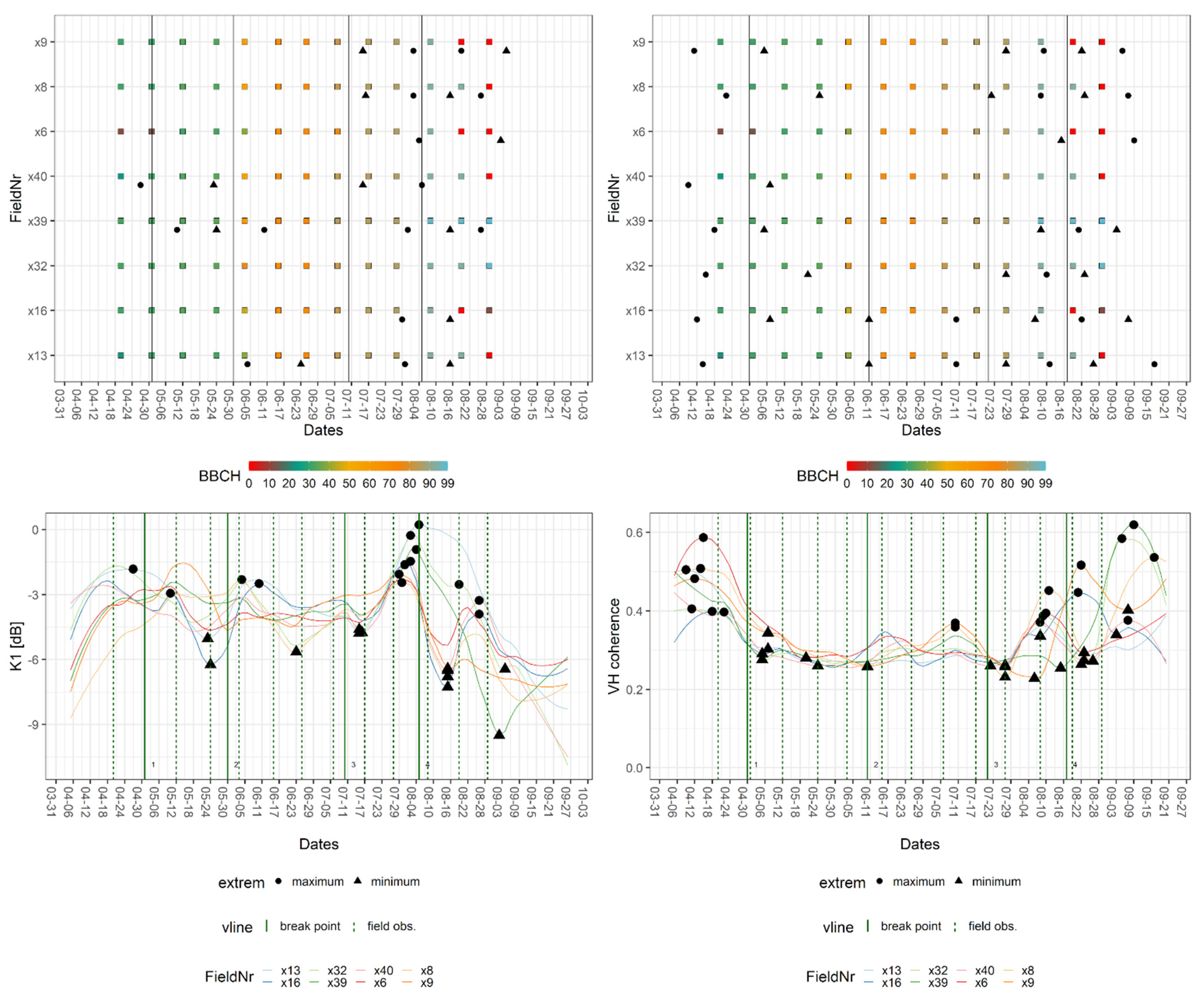
3.2. Signature Analyses

The results for the signature analysis are presented by crop type, including listings of breakpoints and extrema with their corresponding phenological events or stages.

3.2.1. Signatures of Wheat

The breakpoint and extreme value analysis for wheat fields and the crop signatures of K1 and VH coherence are provided in Figure 6. The figure consists of two parts. The upper part shows the BBCH progression of the in situ measurements per field with the dates of relevant extrema (extreme) and breakpoints (vertical line: breakpoint). The lower part depicts the smoothed signatures for each field with their relevant extrema, the breakpoints as well as the dates of their closest field observation (vertical line: field obs.). Here, the high inter-field variance of wheat became visible along with many local extrema, which, in the case of VH coherence, displayed short and distinct intervals. The breakpoints for wheat signatures were close to the following field observations: stem elongation (BBCH: 31–33), inflorescence—heading (BBCH: 57), end of the flowering phase (BBCH: 69), the early stage of fruit development (BBCH: 71), transition from fruit development to ripening (BBCH: 83), ripening/soft dough (BBCH: 85), and early and late stages of senescence (BBCH: 93–99). The S-1 features which exhibited a breakpoint at the given BBCH value are listed in Table 3.
While the beginning of stem elongation was marked by a wide array of features, a later stage could only be detected by VV coherence and backscatter. The end of inflorescence as well as the transition from fruit development to ripening was represented in signatures of the Kennaugh matrix elements and VH backscatter. A later stage of ripening produced breakpoints in both InSAR coherence signatures and Alpha, whereas the onset of senescence was captured by Kennaugh matrix elements and the VH coherence. The harvest or late senescence was covered by breakpoints of VV coherence and Alpha and Entropy. Flowering and fruit development are stages that were present in one or two SAR features only, namely VH coherence and Alpha (flowering) as well as VV backscatter (fruit development).
Local maxima and minima listed in Table 4 were found close to the stages of stem elongation (BBCH: 31), fruit development (BBCH: 71–73), ripening (BBCH: 85/86), and senescence (BBCH: 93). For both metrics, the time difference ranged between zero and five days (i.e., one S-1 repetition cycle). Only the extrema located at the beginning and the end of the time series displayed greater temporal differences (up to 22 days). This was explained by the fact that the S-1 time series encompasses a longer period than the field observations. Since the in situ data did not cover the entire growing season, the tables contain entries labelled as estimated (“est.”). These represent estimated phenological stages based on the natural progression of the plant life cycle described in the literature [28]. A more detailed explanation for this is offered in the discussion section. Due to their small range of values, which exacerbated the distinction of noise and information, K5 and K6 were left out of the analysis of extrema. Additionally, the extrema of the wheat signatures scattered widely (no clumps) around certain time steps and were, therefore, excluded from Table 4.
By combining the breakpoints of VH coherence, Alpha, and VV intensity, detection of the transition from vegetative to the reproductive stage was possible. Considering the temporal difference of breakpoint and observation, the wheat fields completed their transition to the reproductive stage on 24 June 2017. When comparing the detected phases of extrema and breakpoints, a clear distinction between interferometric and polarimetric features was observed. There were no stages that simultaneously produce extrema for polarimetric and interferometric features. Also, the extreme value analysis detected additional phenological events: fruit development (BBCH: 70 and 73) as well as ripening (BBCH: 86), which were indicated by VV backscatter, K0 (BBCH: 70, 73), and VV coherence (BBCH: 86). The largest amount of phenological events were detected by K0 and both backscatters.

3.2.2. Signatures of Canola

The breakpoints within the canola signatures (Table 5) were allocated close to the start, full extent, decline of flowering (BBCH: 60, 65, and 67), middle of fruit development (BBCH: 74), time of harvest, and emergence of secondary vegetation after the harvest. Relevant extrema (Table 6) were located around the start and the decline of flowering (BBCH: 60, 67), the beginning of flowering, and the harvest and the emergence of secondary vegetation. In this case, secondary vegetation refers to the re-emergence of any type of vegetation, for example, green fertilizer or winter cereal. Similar to wheat, the temporal distance ranged between zero and five days for the breakpoints. The extrema exhibited similar behaviour; however, there were also outliers towards the beginning and the end of the observation period, which resulted in a maximal temporal divergence of 24 days. Only the stages of inflorescence emergence (BBCH: 57/58), flowering (BBCH: 60–69), and fruit development (BBCH: 74) were assigned to the breakpoints and extrema within the canola signatures, because of a gap in the GFZ-field data. The lack of data is visible in Figure 7 as zero values between early June and early August; it also demonstrates a characteristic mid-season peak for VH coherence.
Different steps of flowering were distinguished by comparing phases aligned with breakpoints of various S-1 features. The beginning was covered by Alpha and Entropy, K1, K5, and VV backscatter, while the middle of the stage was represented by K6 and VH backscatter, and the later stage produced breakpoints in signatures of both InSAR coherences, K1 and, VV backscatter. Additionally, Alpha and Entropy were the only features with a breakpoint covering the development of fruit. The estimated date of harvest, which was derived from DWD data, was covered by VV and VH coherence and Alpha, whereas the in situ observation of harvested fields produced breakpoints in both backscatter and the Kennaugh matrix elements, except for K6. The onset of secondary vegetation was marked by both InSAR coherences, Alpha and Entropy, VV and VH backscatter, and K0. As observed for wheat, the extrema of canola signatures were less consistent, and the feature groups exhibited a clear disparity in behaviour. For example, Alpha and InSAR coherences were only linked to the harvest and the emergence of secondary vegetation, whereas intensity-based features enable the detection of multiple events. The most phenological events were found in VH backscatter signatures.
The transition from vegetative to reproductive stage was allocated, as the breakpoints of canola signature covered the decline of flowering and the development of fruit. As these breakpoints did not encompass the onset of fruit development, the estimation was less accurate. Nevertheless, a local maximum for K1 was found that covers the point of transition since the lowest BBCH value recorded at that time was 69 and the highest was 73. Using this extremum, the arrival at the reproductive stage was allocated on 4 June 2017. Taking only the breakpoints into account, the estimated dates of transition were 1 June or 2 June 2017. Because the start of flowering was represented as well, the start of the transition was estimated at 1 May 2017, resulting in a transitional period of roughly one month, with the decline of flowering being recorded in situ on 24 May 2017. Incidentally, this event was also represented by breakpoints on 20 May and 21 May 2017.

3.2.3. Signatures of Sugar Beet

Sugar beet was characterised by distinctive signatures in the time series of VV and VH coherence, which reflected its dissimilarity in physiognomy and taxonomy to the other crops. The field data for the sugar beet covered only two phases across the entire observation period: leaf (BBCH: 10; 16/18; 19) and rosette development (BBCH: 33–36; 39). The transition between these two phases was identifiable by employing S-1 features. The breakpoints of sugar beet signatures aligned with both phases. The median BBCH values for the breakpoints covering leaf development were 10, 12, and 19, whereas the values associated with breakpoints within the phase of rosette development were 33 and 39. The extrema displayed similar behaviour, yet VV backscatter exhibited a local minimum that was linked to a BBCH value of 17. Figure 8 displays the breakpoints for K1 at BBCH values of 12 and 33. For VH coherence, the breakpoints cover BBCH values of 10 and 19.
Table 7 lists the breakpoints for each S-1 feature and the corresponding median BBCH-values, whereas Table 8 displays the extrema and their respective BBCH-values. Except for VH coherence, every feature produced a breakpoint for both phenological stages. Leaf development (BBCH: 10) was indicated by VV and VH coherence as well as K6, leaf development (BBCH: 12) by Alpha and Entropy, K0, K1, VH, and VV backscatter. The later leaf development (BBCH: 19) was found in signatures of both coherences, Alpha and Entropy, plus K6. The earlier stage of rosette development (BBCH: 33) produced a breakpoint in K0, K1, K5, and both backscatter signatures, whereas later rosette development (BBCH: 39) was indicated by every feature except the VH coherence.
In addition, the extrema cover leaf development (BBCH 17), which was represented by minima in signatures of K0, and both backscatters. Furthermore, rosette development (BBCH 39) was only covered by K0 and VH backscatter. In sum, the K0 and VH backscatter represented the most phenological events. The transition from the vegetative to the reproductive stage was not detected, because the first year of growth has no flowering phase [28].

4. Discussion

4.1. Elementary Data Analysis

The results of the elementary data analysis provided initial insights into the relationship between SAR-based time series and crop phenology. First, some crops (e.g., wheat), exhibited a higher inter-field variance than others. Therefore, the loss of information by the aggregation to a coarser scale was most likely dependent on the crop type. Second, the pixel-based standard deviation, which was computed for the entire time series, proved to be a valid indicator for the sensitivity of SAR features towards phenological development. It indicated the strong changes in InSAR coherence signatures of sugar beet and the comparatively high sensitivity of backscatter. Third, the influence of plant physiognomy became evident by comparing the standard deviations of VV and VH backscatter, as wheat, whose structure is dominated by vertical elements [55,56,57], exhibited a higher standard deviation than canola, which has a more complex and dense vegetation structure. The latter also produced stronger responses of SAR features, such as Alpha and Entropy, and VH backscatter, which was also confirmed by the signature analysis. Moreover, the physiognomy of wheat served as the first explanation of its higher inter-field variance, because fully grown stems and developing fruits are likely more susceptive to stochastic displacement by wind and precipitation [10].
The results of the correlation analysis revealed multiple statistical redundancies. The high correlations of Alpha and Entropy, as well as backscatter and K0, were explained by the fact that the former pair is derived from dual-polarized data (missing the phase relation between HH and VV) and K0 represented the combined backscatter. The high correlation of K1 and Alpha was related to the fact that K1 is the difference between the complex signals of VV and VH. The lack of strong correlation coefficients (R > |0.7|) between BBCH values and SAR features can be attributed to the difficulty of describing nonlinear developments, such as plant growth or SAR-based time series, with linear trends such as the BBCH scale [14,45].

4.2. Realisations of the Signature Analysis

As demonstrated, breakpoint and extreme value analyses were successfully employed to track phenological development in polarimetric and interferometric time series. K5 and K6 were the SAR features that were less sensitive to phenological development. Because of their sensitivity to deterministic targets, this was an expected result [25]. On the contrary, backscatter and K0 exhibited the strongest dependency on phenological stages or events. Signatures derived from these SAR features generated the most breakpoints and extrema. This is in line with several studies on backscatter and their ratios to monitor phenological development [11,19,55,56]. InSAR coherences, Alpha and Entropy tended towards a binary behaviour, which was often related to strong changes in biomass, for example, harvest or stages of rapid growth. These observations are in line with the results of Khabbazan et al. (2019) [22] and Schlund and Erasmi (2020) [16]. However, it was demonstrated that a more detailed tracking of macro and micro stadia is possible by combining polarimetric and interferometric features. Detailed assessments of each crop type concerning complementary potential are provided below.
The signature analysis of wheat revealed that the following macro stadia produced strong signal responses: stem elongation, inflorescence heading, ripening, and senescence. Flowering and fruit development could only be tracked by two S-1 features and yet these phases match the findings of Khabbazan et al. (2019) [22], who investigated general trends in crop signatures derived from backscatter. The detection of flowering was only achieved by computing VH coherence and Alpha, thus providing a first proof of the complementary value of polarimetric and interferometric S-1 features. Alpha and InSAR coherences also tracked ripening (BBCH 85). When comparing the stages of wheat detected in this study with the results of previous studies, some differences become evident. Schlund and Erasmi (2020) [16] extracted stem elongation (BBCH 31), fruit development (BBCH 75), and ripening (BBCH 87), whereas Meroni et al. (2021) [23] were able to detect stem elongation (BBCH 31) and ripening (BBCH 87). This confirms that stem elongation and ripening create a strong signal response in the C-Band SAR time series, and the additional phase detected by this study indicates that more detailed monitoring of wheat phenology is possible. When applying the definition of most critical stages for wheat development [31,58] as provided by Schlund and Erasmi (2020) [16], this study only detected stem elongation (BBCH 31). Fruit development was only tracked for the BBCH-Values of 70, 71, and 73, whereas values of ripening encompassed 83, 85, and 86. However, if the transition from the vegetative to reproductive stage is classified as the most crucial phase [29,30], the completion of this transition was successfully detected by tracking the end of flowering as well as the start of fruit development.
The definitions of crucial phases used in this study and related research in regard to canola are congruent. According to the literature, developments during the flowering phase of canola are directly linked to the oil content of its seeds [59,60]. The stages detected by the presented approach only partially overlapped with previous observations. D’Andrimont et al. (2020) [21] identified BBCH-values of 61, 65, and 69, whereas Meroni et al. (2021) [23] was only able to detect events corresponding to BBCH values of 61 and 99. This study produced extrema and breakpoints for flowering (BBCH: 60, 65, 67), fruit development (BBCH: 72, 74), and likely harvest dates. As mentioned in Section 4.1, the complex and dense vegetation cover of canola is reflected in its crop signatures. A similar effect was observed by other studies employing SAR data [24,61]. This was especially reflected by the InSAR coherences, which both produced a peak after the onset of the flowering period. Because the in situ data did not cover this period, an estimation based on the progression described by Meier (2001) [28] links this trend to the end of ripening. The harvest period was again represented by field data. Here, an early harvest date was tracked by InSAR coherences and Alpha, whereas the later harvest date was marked by backscatter and K0, K1, and K5. The advantages of combining polarimetric and interferometric features to track the phenological development of canola are, therefore, less evident when compared to wheat. Only fruit development (BBCH: 74) produced exclusive breakpoints for Alpha and Entropy. However, the midseason peak of InSAR coherences and the period between fruit development and harvest are deemed worthy of further investigation.
The signatures of sugar beet offer a better example for the complementary value of polarimetric and interferometric features. Here, leaf development (BBCH: 10 and 19) produce breakpoints and extrema for Alpha and Entropy and InSAR coherences, whereas leaf development (BBCH: 12) and rosette development (BBCH: 33) were tracked by intensity-based features. Rosette development (BBCH: 39), which refers to the closing of the canopy [28], was detected by most features, as the dates of detection of rosette development range from early July to mid-August. Compared to Khabbazan et al. (2019) [22], the presented approach was able to track a more detailed phenological development of sugar beets than emergence and closure by employing breakpoint and extreme value analysis of multiple S-1 features, instead of slope analysis based on InSAR coherences only.
The SAR-based signatures of all crop types indicated that the quality of the results depends on the smoothing algorithm. Schlund and Erasmi (2020) [16] also used LOESS, but they applied a one-degree polynomial model instead of a linear model and set a different span. This may already partly explain the disparity in detected events. Other smoothing approaches encompass harmonic time series analysis [20] or a Whittaker fit [21]. Hence, the comparability of these studies is already impaired and the SAR feature that produced the most breakpoints and extrema might be dependent on the choice of smoothing approach. K5 and K6, for example, would be less indicative of phenological changes if their signatures become more generalised. Nevertheless, the difference in time between detection and in situ observation is somewhat comparable. Here, a range from zero to five days matches the findings of other studies [16,23]. Various types of fitting also introduce a different number of extrema, which have to be addressed by filtering out extrema not related to phenological development [23]. Despite this issue, extrema enabled the tracking of additional phenological stages and events.
A definite limit of this approach is the saturation of features, such as InSAR coherences, or Alpha and Entropy. These features are only capable of reflecting certain parts of phenological development. Once the plants are grown to a certain extent, the temporal decorrelation becomes too strong (InSAR coherence), or the depolarisation is maximized (Entropy). Therefore, backscatter are crucial for successful phenology monitoring because VV and VH reflect different stages of the plant development, such a fruit development and ripening of wheat [16,22].

5. Conclusions

In this study, time series (April–September 2017) of several polarimetric and interferometric features of Sentinel-1 were used to identify the phenological phases and crucial stages of plant development of three crop types (wheat, canola, and sugar beet). It was found that temporal SAR signatures of wheat are mainly influenced by the stem elongation, inflorescence/heading, ripening, and senescence, whereas, for sugar beet, S-1 features were sensitive to the leaf and rosette development. Flowering and fruit development of canola were revealed in the temporal signatures, yet other stages could not be identified due to the lack of in situ data. These findings confirm the results of related studies [16,21,22,23] and offer further details of crop phenological development, as multiple micro stadia of the leaf development of sugar beets, the flowering of canola, as well as the ripening and senescence of wheat, were tracked. This degree of detail is ascribed to the combined usage of polarimetric and interferometric SAR features.
It is suggested that future research is directed towards multi-annual frameworks. Hereby, the robustness across multiple growing seasons should be assessed, especially for extremely dry or wet seasons [16]. In addition, these endeavours should be accompanied by elaborate fieldwork to further investigate the potential and reliability of SAR-based phenology monitoring at the field or even sub-field level [23,24]. Furthermore, the influence of various smoothing approaches on the tracking of phenological development needs to be researched, to avoid an issue that is comparable to deriving crop phenology from various optical sensors [62].

Author Contributions

Conceptualization, J.L. and T.U.; Data curation, J.L. and T.U.; Formal Analysis, J.L.; Software, J.L. and T.U.; Investigation, J.L.; Methodology, J.L. and T.U.; Resources, C.C.; Supervision, T.U. and C.C.; Validation: J.L., T.U. and C.C.; Visualization: J.L. and T.U.; Writing—original draft, J.L.; Writing—review and editing, T.U. and C.C. All authors have read and agreed to the published version of the manuscript.

Funding

This research received no external funding.

Data Availability Statement

Publicly available datasets were analyzed in this study. Sentinel-1 data can be found here: https://scihub.copernicus.eu/ (accessed on 10 June 2021). Phenological data provided by DWD is available at: https://cdc.dwd.de/portal/ (accessed on 10 June 2021). In-situ data and resulting data sets presented in this study are available on request from the corresponding author.

Acknowledgments

We would like to thank Daniel Spengler GFZ for providing us with in situ data. Additionally, we would like to thank ESA for providing the Sentinel-1 data and DWD for their data on phenology.

Conflicts of Interest

The authors declare no conflict of interest.

References

  1. Lieth, H. (Ed.) Phenology and Seasonality Modeling; Springer: New York, NY, USA, 1974; ISBN 9783642518652. [Google Scholar]
  2. Gao, F.; Anderson, M.C.; Zhang, X.; Yang, Z.; Alfieri, J.G.; Kustas, W.P.; Mueller, R.; Johnson, D.M.; Prueger, J.H. Toward mapping crop progress at field scales through fusion of Landsat and MODIS imagery. Remote Sens. Environ. 2017, 188, 9–25. [Google Scholar] [CrossRef] [Green Version]
  3. Stathers, T.; Lamboll, R.; Mvumi, B.M. Postharvest agriculture in changing climates: Its importance to African smallholder farmers. Food Secur. 2013, 5, 361–392. [Google Scholar] [CrossRef]
  4. Sakamoto, T.; Gitelson, A.A.; Arkebauer, T.J. MODIS-based corn grain yield estimation model incorporating crop phenology information. Remote Sens. Environ. 2013, 131, 215–231. [Google Scholar] [CrossRef]
  5. Steele-Dunne, S.C.; McNairn, H.; Monsivais-Huertero, A.; Judge, J.; Liu, P.W.; Papathana, K. Radar Remote Sensing of Agriciltural Canopies. IEEE J. Sel. Top. Appl. Earth Obs. Remote Sens. 2017, 10, 2249–2273. [Google Scholar] [CrossRef] [Green Version]
  6. Ulaby, F.; Moore, R. Radar sensing of soil moisture. In Proceedings of the 1973 Antennas and Propagation Society International Symposium, Boulder, CO, USA, 22–24 April 1973; Volume 11, pp. 362–365. [Google Scholar]
  7. Ulaby, F. Radar response to vegetation. IEEE Trans. Antennas Propag. 1975, 23, 36–45. [Google Scholar] [CrossRef]
  8. Weise, K.; Davidson, M.W.J. Dualband—TerraSAR simulation/campaign results for L-band configuration. In Proceedings of the IGARSS 2004 IEEE International Geoscience and Remote Sensing Symposium, Anchorage, AK, USA, 20–24 September 2004; Volume 7, pp. 4556–4559. [Google Scholar]
  9. Su, Z.; Timmermans, W.J.; van der Tol, C.; Dost, R.; Bianchi, R.; Gómez, J.A.; House, A.; Hajnsek, I.; Menenti, M.; Magliulo, V.; et al. EAGLE 2006—Multi-purpose, multi-angle and multi-sensor in-situ and airborne campaigns over grassland and forest. Hydrol. Earth Syst. Sci. 2009, 13, 833–845. [Google Scholar] [CrossRef]
  10. Wegmüller, U.; Werner, C. Farmland monitoring with SAR interferometry. Geosci. Remote Sens. Symp. 1995, 1, 544–546. [Google Scholar]
  11. Baghdadi, N.; Boyer, N.; Todoroff, P.; El Hajj, M.; Bégué, A. Potential of SAR sensors TerraSAR-X, ASAR/ENVISAT and PALSAR/ALOS for monitoring sugarcane crops on Reunion Island. Remote Sens. Environ. 2009, 113, 1724–1738. [Google Scholar] [CrossRef]
  12. Mascolo, L.; Lopez-Sanchez, J.M.; Vicente-Guijalba, F.; Mazzarella, G.; Nunziata, F.; Migliaccio, M. Retrieval of phenological stages of onion fields during the first year of growth by means of C-band polarimetric SAR measurements. Int. J. Remote Sens. 2015, 36, 3077–3096. [Google Scholar] [CrossRef] [Green Version]
  13. Cloude, S.R.; Pottier, E. A review of target decomposition theorems in radar polarimetry. IEEE Trans. Geosci. Remote Sens. 1996, 34, 498–518. [Google Scholar] [CrossRef]
  14. Canisius, F.; Shang, J.; Liu, J.; Huang, X.; Ma, B.; Jiao, X.; Geng, X.; Kovacs, J.M.; Walters, D. Tracking crop phenological development using multi-temporal polarimetric Radarsat-2 data. Remote Sens. Environ. 2018, 210, 508–518. [Google Scholar] [CrossRef]
  15. Ndikumana, E.; Ho Tong Minh, D.; Baghdadi, N.; Courault, D.; Hossard, L. Deep Recurrent Neural Network for Agricultural Classification using multitemporal SAR Sentinel-1 for Camargue, France. Remote Sens. 2018, 10, 1217. [Google Scholar] [CrossRef] [Green Version]
  16. Schlund, M.; Erasmi, S. Sentinel-1 time series data for monitoring the phenology of winter wheat. Remote Sens. Environ. 2020, 246, 111814. [Google Scholar] [CrossRef]
  17. Torres, R.; Snoeij, P.; Geudtner, D.; Bibby, D.; Davidson, M.; Attema, E.; Potin, P.; Rommen, B.; Floury, N.; Brown, M.; et al. GMES Sentinel-1 mission. Remote Sens. Environ. 2012, 120, 9–24. [Google Scholar] [CrossRef]
  18. Ruml, M.; Vulic, T. Importance of phenological observations and predictions in agriculture. J. Agric. Sci. Belgrade 2005, 50, 217–225. [Google Scholar] [CrossRef]
  19. Wali, E.; Tasumi, M.; Moriyama, M. Combination of linear regression lines to understand the response of sentinel-1 dual polarization SAR data with crop phenology-case study in Miyazaki, Japan. Remote Sens. 2020, 12, 189. [Google Scholar] [CrossRef] [Green Version]
  20. Song, Y.; Wang, J. Mapping winter wheat planting area and monitoring its phenology using Sentinel-1 backscatter time series. Remote Sens. 2019, 11, 449. [Google Scholar] [CrossRef] [Green Version]
  21. D’Andrimont, R.; Taymans, M.; Lemoine, G.; Ceglar, A.; Yordanov, M.; van der Velde, M. Detecting flowering phenology in oil seed rape parcels with Sentinel-1 and -2 time series. Remote Sens. Environ. 2020, 239, 111660. [Google Scholar] [CrossRef]
  22. Khabbazan, S.; Vermunt, P.; Steele-Dunne, S.; Arntz, L.R.; Marinetti, C.; van der Valk, D.; Iannini, L.; Molijn, R.; Westerdijk, K.; van der Sande, C. Crop monitoring using Sentinel-1 data: A case study from The Netherlands. Remote Sens. 2019, 11, 1887. [Google Scholar] [CrossRef] [Green Version]
  23. Meroni, M.; d’Andrimont, R.; Vrieling, A.; Fasbender, D.; Lemoine, G.; Rembold, F.; Seguini, L.; Verhegghen, A. Comparing land surface phenology of major European crops as derived from SAR and multispectral data of Sentinel-1 and -2. Remote Sens. Environ. 2021, 253. [Google Scholar] [CrossRef]
  24. Shang, J.; Liu, J.; Poncos, V.; Geng, X.; Qian, B.; Chen, Q.; Dong, T.; Macdonald, D.; Martin, T.; Kovacs, J.; et al. Detection of crop seeding and harvest through analysis of time-series Sentinel-1 interferometric SAR data. Remote Sens. 2020, 12, 1551. [Google Scholar] [CrossRef]
  25. Schmitt, A.; Wendleder, A.; Hinz, S. The Kennaugh element framework for multi-scale, multi-polarized, multi-temporal and multi-frequency SAR image preparation. ISPRS J. Photogramm. Remote Sens. 2015, 102, 122–139. [Google Scholar] [CrossRef] [Green Version]
  26. Verbesselt, J.; Zeileis, A.; Herold, M. Near real-time disturbance detection using satellite image time series. Remote Sens. Environ. 2012, 123, 98–108. [Google Scholar] [CrossRef]
  27. Verbesselt, J.; Hyndman, R.; Zeileis, A.; Culvenor, D. Phenological change detection while accounting for abrupt and gradual trends in satellite image time series. Remote Sens. Environ. 2010, 114, 2970–2980. [Google Scholar] [CrossRef] [Green Version]
  28. Meier, U. Growth Stages of Mono-and Dicotyledonous Plants. BBCH Monograph, 2nd ed.; Meier, U., Ed.; Federal Biological Research Centre for Agriculture and Forestry: Berlin/Braunschweig, Germany, 2001. [Google Scholar]
  29. Bastidas, A.M.; Setiyono, T.D.; Dobermann, A.; Cassman, K.G.; Elmore, R.W.; Graef, G.L.; Specht, J.E. Soybean sowing date: The vegetative, reproductive, and agronomic impacts. Crop Sci. 2008, 48, 727–740. [Google Scholar] [CrossRef] [Green Version]
  30. Araki, T. Transition from vegetative to reproductive phase. Curr. Opin. Plant Biol. 2001, 4, 63–68. [Google Scholar] [CrossRef]
  31. Conradt, S.; Finger, R.; Spörri, M. Climate Risk Management Flexible weather index-based insurance design. Clim. Risk Manag. 2015, 10, 106–117. [Google Scholar] [CrossRef] [Green Version]
  32. Borg, E.; Lippert, K.; Zabel, E.; Löpmeier, F.-J.; Fichtelmann, B.; Jahncke, D.; Maass, H. DEMMIN Teststandort zur Kalibrierung und Validierung von Fernerkundungsmissionen; DLR Eigenverlag: Neustrelitz, Germany, 2009. [Google Scholar]
  33. Spengler, D.; Itzerott, S.; Ahmadian, N.; Borg, E.; Hüttich, C.; Maass, H.; Missling, K.-D.; Schmullius, C.; Truckenbrodt, S.; Conrad, C. The German JECAM site DEMMIN: Status and future perspectives. In Proceedings of the Annual JECAM Meeting, Taichung City, Taiwan, 17–20 September 2018. [Google Scholar]
  34. Team, S. Sentinel-1 User Handbook; ESA Communications: Noordwijk, The Netherlands, 2013. [Google Scholar]
  35. Ullmann, T.; Serfas, K.; Büdel, C.; Padashi, M.; Baumhauer, R. Data Processing, Feature Extraction, and Time-Series Analysis of Sentinel-1 Synthetic Aperture Radar (SAR) Imagery: Examples from Damghan and Bajestan Playa (Iran). Z. für Geomorphol. Suppl. Issues 2019, 62, 9–39. [Google Scholar] [CrossRef]
  36. Ullmann, T.; Sauerbrey, J.; Hoffmeister, D.; May, S.M.; Baumhauer, R.; Bubenzer, O. Assessing spatiotemporal variations of sentinel-1 InSAR coherence at different time scales over the atacama desert (Chile) between 2015 and 2018. Remote Sens. 2019, 11, 2960. [Google Scholar] [CrossRef] [Green Version]
  37. Small, D. Flattening Gamma: Radiometric Terrain Correction for SAR Imagery. IEEE Trans. Geosci. Remote Sens. 2011, 49, 3081–3093. [Google Scholar] [CrossRef]
  38. Richards, J.A. Remote Sensing with Imaging Radar; Springer: Berlin/Heidelberg, Germany, 2009; ISBN 9780387765679. [Google Scholar]
  39. Zhang, Z.; Wang, C.; Zhang, H.; Tang, Y.; Liu, X. Analysis of Permafrost Region Coherence Variation in the Qinghai–Tibet Plateau with a High-Resolution TerraSAR-X Image. Remote Sens. 2018, 10, 298. [Google Scholar] [CrossRef] [Green Version]
  40. Pichierri, M.; Hajnsek, I.; Zwieback, S.; Rabus, B. On the potential of Polarimetric SAR Interferometry to characterize the biomass, moisture and structure of agricultural crops at L-, C- and X-Bands. Remote Sens. Environ. 2018, 204, 596–616. [Google Scholar] [CrossRef]
  41. Scheuchl, B.; Ullmann, T.; Koudogbo, F. Change Detection Using High Resolution TerraSAR-X Data Preliminary Results. In Proceedings of the ISPRS Hannover Workshop 2009, Hannover, Germany, 2–5 June 2009. [Google Scholar]
  42. Zebker, H.A.; Villasenor, J. Decorrelation in interferometric radar echoes. IEEE Trans. Geosci. Remote Sens. 1992, 30, 950–959. [Google Scholar] [CrossRef] [Green Version]
  43. Esch, S. Determination of Soil Moisture and Vegetation Parameters from Spaceborne C-Band SAR on Agricultural Areas. Ph.D. Thesis, Universität zu Köln, Cologne, Germany, 2018. [Google Scholar]
  44. Lee, J.-S.; Pottier, E. Polarimetric Radar Imaging: From Basics to Applications; CRC Press: Boca Raton, FL, USA, 2009; ISBN 9781420054989. [Google Scholar]
  45. Harfenmeister, K.; Itzerott, S.; Weltzien, C.; Spengler, D. Agricultural Monitoring Using Polarimetric Decomposition Parameters of Sentinel-1 Data. Remote Sens. 2021, 13, 575. [Google Scholar] [CrossRef]
  46. Zhang, Y.; Liu, X.; Su, S.; Wang, C. Retrieving canopy height and density of paddy rice from Radarsat-2 images with a canopy scattering model. Int. J. Appl. Earth Obs. Geoinf. 2014, 28, 170–180. [Google Scholar] [CrossRef]
  47. Cleveland, W.S. Robust Locally Weighted Regression and Smoothing Scatterplots Robust Locally Weighted Regression and Smoothing Scatterplots. J. Am. Stat. Assoc. 1979, 74, 829–836. [Google Scholar] [CrossRef]
  48. Cai, Z.; Jönsson, P.; Jin, H.; Eklundh, L. Performance of smoothing methods for reconstructing NDVI time-series and estimating vegetation phenology from MODIS data. Remote Sens. 2017, 9, 1271. [Google Scholar] [CrossRef] [Green Version]
  49. Nagendra, H.; Rocchini, D.; Ghate, R.; Sharma, B.; Pareeth, S. Assessing plant diversity in a dry tropical forest: Comparing the utility of landsat and ikonos satellite images. Remote Sens. 2010, 2, 478–496. [Google Scholar] [CrossRef] [Green Version]
  50. Wickham, H.; Averick, M.; Bryan, J.; Chang, W.; McGowan, L.D.; François, R.; Grolemund, G.; Hayes, A.; Henry, L.; Hester, J.; et al. Welcome to the Tidyverse. J. Open Source Softw. 2019, 4, 1686. [Google Scholar] [CrossRef]
  51. R Core Team. A Language and Environment for Statistical Computing. Available online: https://www.R-project.org/ (accessed on 10 June 2021).
  52. Bai, J.; Perron, P. Computation and analysis of multiple structural change models. J. Appl. Econom. 2003, 18, 1–22. [Google Scholar] [CrossRef] [Green Version]
  53. Zeileis, A.; Kleiber, C.; Krämer, W.; Hornik, K. Testing and dating of structural changes in practice. Comput. Stat. Data Anal. 2003, 44, 109–123. [Google Scholar] [CrossRef] [Green Version]
  54. Wu, Z.; Huang, N. Ensemble Empirical Mode Decomposition: A Noise-Assisted Data Analysis Method. Adv. Data Sci. Adapt. Anal. 2009, 1, 1–41. [Google Scholar] [CrossRef]
  55. Veloso, A.; Mermoz, S.; Bouvet, A.; Le Toan, T.; Planells, M.; Dejoux, J.F.; Ceschia, E. Understanding the temporal behavior of crops using Sentinel-1 and Sentinel-2-like data for agricultural applications. Remote Sens. Environ. 2017, 199, 415–426. [Google Scholar] [CrossRef]
  56. Vreugdenhil, M.; Wagner, W.; Bauer-Marschallinger, B.; Pfeil, I.; Teubner, I.; Rüdiger, C.; Strauss, P. Sensitivity of Sentinel-1 backscatter to vegetation dynamics: An Austrian case study. Remote Sens. 2018, 10, 1396. [Google Scholar] [CrossRef] [Green Version]
  57. Mattia, F.; Le Toan, T.; Picard, G.; Posa, F.I.; Alessio, A.D.; Notarnicola, C.; Gatti, A.M.; Rinaldi, M.; Satalino, G. Multitemporal C-Band Radar Measurements on Wheat Fields. IEEE Trans. Geosci. Remote Sens. 2003, 41, 1551–1560. [Google Scholar] [CrossRef]
  58. Möller, M.; Gerstmann, H.; Gao, F.; Christian, T.; Förster, M. Catena Coupling of phenological information and simulated vegetation index time series: Limitations and potentials for the assessment and monitoring of soil erosion risk. Catena 2017, 150, 192–205. [Google Scholar] [CrossRef]
  59. Kirkegaard, J.A.; Lilley, J.M.; Brill, R.D.; Ware, A.H.; Walela, C.K. Field Crops Research The critical period for yield and quality determination in canola (Brassica napus L.). Field Crop. Res. 2018, 222, 180–188. [Google Scholar] [CrossRef]
  60. Zhang, H.; Flottmann, S. Source-sink manipulations indicate seed yield in canola is limited by source availability. Eur. J. Agron. 2018, 96, 70–76. [Google Scholar] [CrossRef]
  61. McNairn, H.; Jiao, X.; Pacheco, A.; Sinha, A.; Tan, W.; Li, Y. Estimating canola phenology using synthetic aperture radar. Remote Sens. Environ. 2018, 219, 196–205. [Google Scholar] [CrossRef]
  62. Younes, N.; Joyce, K.E.; Maier, S.W. All models of satellite-derived phenology are wrong, but some are useful: A case study from northern Australia. Int. J. Appl. Earth Obs. Geoinf. 2021, 97, 102285. [Google Scholar] [CrossRef]
Figure 1. Map of the study area and the locations of the observed fields; background: false-colour composite of Sentinel-2 with a band combination of 4-3-2.
Remotesensing 13 02951 g001
Figure 2. Development of daily mean air temperature [°C] and daily precipitation [mm] for the growing season of 2017, and acquisition dates of field sampling and Sentinel-1.
Remotesensing 13 02951 g002
Figure 3. Exemplary smoothing of wheat signatures for Alpha (left) and VV backscatter (right) using the locally weighted scatterplot smoothing (LOESS) algorithm.
Remotesensing 13 02951 g003
Figure 4. Correlation heatmap of wheat fields covered by this study showing potential information redundancies and statistically relevant relations.
Remotesensing 13 02951 g004
Figure 5. Crop-specific standard deviations for VV backscatter (VV [dB]), VH backscatter (VH [dB]), VH coherence (VH Coh), Alpha (ALP [°]), and K0 [dB] for canola (orange), grassland (dark green), sugar beet (brown), and wheat (green), as well as VH coherence mean and standard deviation [dB], and a subset of the original measurement points as a background image.
Remotesensing 13 02951 g005
Figure 6. Exemplary breakpoint and extreme value analysis for K1 and VH coherence signatures of fields of wheat. Upper part: BBCH progression of in situ measurements per field with dates of breakpoints (vertical line = breakpoint) and relevant extrema (extreme). Lower part: crop signatures with breakpoints and relevant extrema as well as dates of closest field observations (vertical line = field obs.).
Remotesensing 13 02951 g006
Figure 7. Exemplary breakpoint and extreme value analysis for K1 and VH coherence signatures of fields of canola. Upper part: BBCH progression of in situ measurements per field with dates of breakpoints (vertical line = breakpoint) and extrema (extreme). Lower part: crop signatures with breakpoints and extrema as well as dates of closest field observations (vertical line = field obs.).
Remotesensing 13 02951 g007
Figure 8. Exemplary breakpoint and extreme value analysis for K1 and VH coherence signatures of sugar beet fields. Upper part: BBCH progression of in situ measurements per field with dates of breakpoints (vertical line = breakpoint) and extrema (extreme). Lower part: crop signatures with breakpoints and extrema as well as dates of closest field observations (vertical line = field obs.).
Remotesensing 13 02951 g008
Table 1. Information on phenological events in 2017 provided by the DWD per station (with ID).
Wheat
DWD label1215182124
BBCH stage-MainshootHeadingRipeningHarvest
Dargun: 12615-10 April 20174 June 201723 July 20176 August 2017
Gülzow: 12563-20 April 20173 June 2017-4 August 2017
Tützpatz: 12508-2 May 201731 May 201712 July 20174 August 2017
Canola
DWD label710121724
BBCH stageEnd of FloweringPreparing FieldGermationBud developmentHarvest
Dargun: 1261529 May 201717 August 201725 August 201730 March 20174 August 2017
Gülzow: 1256330 May 201723 August 201730 August 201720 March 201724 July 2017
Tützpatz: 1250829 May 201719 August 20172 September 20174 April 201726 July 2017
Table 2. Computed Sentinel-1 features, their abbreviations, units, and interpretation. Dimensionless features are labelled as such by “/” in the column “Unit”.
FeatureAbbreviationUnitAbout
VV coherenceVV Coh/InSAR coherence in VV of two consecutive acquisitions *
VH coherenceVH Coh/InSAR coherence in VH of two consecutive acquisitions *
AlphaALPDegree [°]Relation of VV and VH simulating the dominant scattering mechanism
EntropyENT/Degree of depolarisation
Kennaugh element K0K0dBCombined backscatter (VV + VH)
Kennaugh element K1K1dBDifference in backscatter (VV − VH)
Kennaugh element K5K5dBReal part of inter-channel correlation between VV and VH
Kennaugh element K6K6dBImaginary part of inter-channel-correlation between VV and VH
VV backscatterVVdBGamma nought VV intensity in dB
VH backscatterVHdBGamma nought VH intensity in dB
* six-day temporal baselines and absolute perpendicular baselines <200 m.
Table 3. Median BBCH values and phenological stages of breakpoints derived from Sentinel-1 (S-1) features in wheat fields.
Phenological StagesMedian BBCH Value at BreakpointBreakpoint Producing SAR Features
Stem elongation31VH coh, ALP, ENT, K0, K1, K5, K6 VH int, VV int
Stem elongation33VV coh, VV int
Inflorescence/Heading57K0, K1, K5, K6, VH int
Flowering69VH coh, ALP
Fruit development71VV int
Ripening83K0, K1, K5, K6, VH int
Ripening85VH coh, VV coh, ALP
Senescence93VH coh, K0, K1, K5, K6
Senescence99VV coh, ALP, ENT
Table 4. Summary of relevant extrema and corresponding BBCH values for wheat signatures.
Phenological StageMedian BBCH ValueSAR Feature Producing MinimumSAR Feature Producing Maximum
Est. Tillering -VH coh
Stem elongation31VH cohVH int, VV int
Fruit development70-VV int, K0
Fruit development71VH int-
Fruit development73VV int, K0-
Ripening85-VV int
Ripening86VV cohVH int, K0
Senescence93VH int, VV int, K0VH int
Table 5. Median BBCH values and phenological stages of breakpoints derived from corresponding SAR features in canola fields.
Phenological StagesMedian BBCH Value at BreakpointBreakpoint Producing SAR Features
Flowering60ALP, ENT, K1, K5, VV int
Flowering65K6, VH int
Flowering67VH coh, VV coh, K1, VV int
Fruit development74ALP, ENT
Est. harvest-VH coh, VV coh, ALP
Harvested-K0, K1, K5, VV int, VH int
Harvested, secondary Vegetation-VH coh, VV coh, ALP, ENT, K0, VH int, VV int
Table 6. Summary of relevant extrema and corresponding BBCH values for canola signatures.
Phenological StageMedian BBCH ValueSAR Feature Producing MinimumSAR Feature Producing Maximum
Flowering:60-K0, VH int
Flowering:67K0, VH int-
Fruit development:72VH intK1
Est. harvest--K1, ALP
Harvest-VH coh, VV coh, K0, VH int, VV int-
Secondary vegetationVH coh, K0, VH int, VV int--
Table 7. Median BBCH values and phenological stages of breakpoints derived from corresponding SAR features in sugar beet fields.
Phenological StagesMedian BBCH Value at BreakpointBreakpoint Producing SAR Features
Leaf development10VH coh, VV coh, K6
Leaf development12ALP, ENT, K0, K1, VH int, VV int
Leaf development19VH coh, VV coh, ALP, ENT, K6
Rosette development33K0, K1, K5, VV int, VH int
Rosette development39VV coh, ALP, ENT, K0, K1, K5, K6, VV int, VH int
Table 8. Summary of relevant extrema and corresponding BBCH values for sugar beet signatures.
Phenological StageMedian BBCH ValueSAR Feature Producing MinimumSAR Feature Producing Maximum
Leaf development10-VH coh, VV coh
Leaf development12-K0, VH int, VV int
Leaf development17K0, VH int, VV int-
Leaf development19VH coh, VV cohALP, ENT
Rosette development33-K0, K1, VH int, VV int
Rosette development39K0, VH int-
Publisher’s Note: MDPI stays neutral with regard to jurisdictional claims in published maps and institutional affiliations.

