Article

Combining Spectral and Texture Features of UAV Images for the Remote Estimation of Rice LAI throughout the Entire Growing Season

1
School of Remote Sensing and Information Engineering, Wuhan University, Wuhan 430079, China
2
Lab of Remote Sensing for Precision Phenomics of Hybrid Rice, Wuhan University, Wuhan 430079, China
3
College of Life Sciences, Wuhan University, Wuhan 430079, China
*
Author to whom correspondence should be addressed.
Remote Sens. 2021, 13(15), 3001; https://doi.org/10.3390/rs13153001
Submission received: 25 June 2021 / Revised: 25 July 2021 / Accepted: 27 July 2021 / Published: 30 July 2021
(This article belongs to the Special Issue Advances in Remote Sensing for Crop Monitoring and Yield Estimation)

Abstract

:
Leaf area index (LAI) estimation is very important, and not only for canopy structure analysis and yield prediction. The unmanned aerial vehicle (UAV) serves as a promising solution for LAI estimation due to its great applicability and flexibility. At present, vegetation index (VI) is still the most widely used method in LAI estimation because of its fast speed and simple calculation. However, VI only reflects the spectral information and ignores the texture information of images, so it is difficult to adapt to the unique and complex morphological changes of rice in different growth stages. In this study we put forward a novel method by combining the texture information derived from the local binary pattern and variance features (LBP and VAR) with the spectral information based on VI to improve the estimation accuracy of rice LAI throughout the entire growing season. The multitemporal images of two study areas located in Hainan and Hubei were acquired by a 12-band camera, and the main typical bands for constituting VIs such as green, red, red edge, and near-infrared were selected to analyze their changes in spectrum and texture during the entire growing season. After the mathematical combination of plot-level spectrum and texture values, new indices were constructed to estimate rice LAI. Comparing the corresponding VI, the new indices were all less sensitive to the appearance of panicles and slightly weakened the saturation issue. The coefficient of determination (R2) can be improved for all tested VIs throughout the entire growing season. The results showed that the combination of spectral and texture features exhibited a better predictive ability than VI for estimating rice LAI. This method only utilized the texture and spectral information of the UAV image itself, which is fast, easy to operate, does not need manual intervention, and can be a low-cost method for monitoring crop growth.

Graphical Abstract

1. Introduction

As one of the world’s three major food crops, rice is the staple food for half of the global population [1,2,3]. Its leaves, as the main organ of photosynthesis, have a significant effect on the overall growth status of the rice. Leaf area index (LAI), a concept first put forward by Watson [4], is half of the amount of leaf area per unit horizontal ground surface area [4,5,6]. It is regarded as a critical vegetation structural variable that characterizes the geometry of the crop canopy [7,8] and can be used as a predictor in crop biomass and yield estimation [9,10,11]. Accurate estimation of LAI is of great significance to paddy field management and precision agriculture. It is also a key indicator of photosynthesis [12,13] and evapotranspiration [14], and therefore plays an essential role in biogeochemical cycles in ecosystems [15].
With the development of remote sensing technology, the use of remote sensing images to estimate LAI has become a hot topic [5,6]. Past research has involved a variety of remote sensing techniques to estimate LAI based on empirical models [8,10,16,17,18,19] and physical models [20,21,22,23]. The physical model simulates the radiative transfer of the signal within a canopy, but it requires many input parameters [20,21,24] and a few studies have shown that the derived products are less accurate than those of the empirical models [6,25,26]. The other common strategy used to estimate LAI is to establish an empirical relationship between ground measured LAI and vegetation index (VI) [19,27]. Since Rouse used ratio vegetation index (RVI) and normalized difference vegetation index (NDVI) to estimate crop characteristics in the 1970s [28], many VIs based on the combination of reflectance between different wavelengths have been established to estimate LAI in many vegetation types. For example, Viña et al. [29] evaluated several VIs calculated by green, red, red edge, and near-infrared (NIR) bands recorded by radiometers mounted on a ground system for estimating green LAI of maize and soybean in Lincoln, NE, U.S.A.. Yao et al. [17] developed a winter wheat LAI model with modified triangular vegetation index (MTVI2) based on a six-channel narrowband multispectral camera (Mini-MCA6) mounted on unmanned aerial vehicles (UAV) to increase the sensitivity of the model under various LAI values. Qiao et al. [8] chose NDVI to obtain the piecewise LAI-VI relationships based on phenophases of forests, crops, and grasslands using MODIS data. Dong et al. [19] compared the potential of red edge-based and visible-based reflectance VIs, which were calculated from multitemporal RapidEye images, for spring wheat and canola LAI estimation. VI combines the different responses of vegetation under different waveband reflectivity to distinguish the vegetation foreground from the soil background. The method is simple and effectively implemented to estimate phenotypic traits. However, there remain problems to be solved in rice LAI estimation.
The life cycle of rice plants ranges from three to six months from germination to maturity, depending on the variety and environment [30]. There are three main stages of the growth period: vegetative (germination to panicle initiation), reproductive (panicle initiation to heading), and ripening (heading to maturity) [31]. The morphological changes of rice and other vegetation types in different stages are very different. Rice seeds germinate and are then transplanted in soil/water. During vegetative and reproductive stages, with the tillering and jointing of the rice plant, the canopy closes gradually, the leaf area increases sharply, and the background is increasingly occluded. When 50% of the panicles have partially exserted from the leaf sheath, the plant enters heading stage [30,31]. The shape of the rice panicle is thin and long and the surface is rough. From this point on, the grain increases in size and weight and the plant enters ripening stage. With maturity, the panicle changes color from green to gold and turns heavy and droopy, which increases the complexity of the canopy structure. As such, the morphological changes of rice plants at different growth stages are more complex than those of other types of vegetation. It has been proven that the canopy light distribution will change dramatically with the emergence of panicles [32]. The complex changes of rice phenology affect the accuracy of LAI estimation by remote sensing methods during the rice growth season. Sakamoto et al. [33] investigated the relationship between visible atmospherically resistant index (VARI) and rice LAI in the entire growing season. They found that the appearance of yellow panicles in the camera’s field of view would affect the LAI estimation with VARI [33]. Wang et al. [34] used ten VIs to estimate rice LAI before and after heading stages, which also proved that the relationship between LAI and post-heading VIs was weaker than pre-heading VIs.
Some rice LAI estimation experiments used partial samples for prediction before heading, while some made separate predictions of pre- and post-heading stages. Li et al. [35] applied a normalized texture index based on gray level co-occurrence matrix (GLCM) to improve the method of using color indices to estimate rice LAI during tillering to booting stages. Sakamoto et al. [33] established a linear regression model of the relationship between VARI and LAI when LAI was greater than 0.4 before heading. Casanova et al. [16] fitted the rice LAI of the entire growing season with three exponential piecewise functions. The coefficients of determination (R2) could reach 0.7 during vegetation and reproductive stages but only 0.25 during the ripening stage [16]. It must be noted that it is not easy to ascertain the heading date, especially for the experimental fields for breeding. For example, in the study of Ma et al. [36], six rice fields with multiple cultivars distributed in China were studied, and more than 1000 rice cultivars were planted in one single field among them. It is a time-consuming and labor-consuming task for professionals to observe whether these fields are heading every day. Therefore, even if there are many challenges, it is necessary to estimate rice LAI in the entire growing season.
In addition to spectral features, remote sensing images also provide more abundant texture information related to vegetation growth [37]. Zhang et al. [38] combined object-based texture features with a neural network to improve the accuracy of vegetation mapping. It has also been proven that GLCM features of high-resolution images could improve LAI and biomass estimation of forests [39,40]. With the improvement of spectral and spatial resolution of remote sensing images, the potential of texture application is also increasing. Since local binary pattern (LBP) was proposed by Ojala in 1996 [41], it has been considered one of the most effective, prominent, and widely studied local descriptors [42,43]. Due to its computational simplicity and tolerance against illumination changes [44], LBP and its extension have been widely applied in image processing, including texture classification [45,46,47], face recognition [48,49], medical image analysis [50,51,52], and archaeological surveying [53]. Compared with the GLCM method, the LBP operator is better at describing micro texture [54], and its ability to analyze multiple pixels at one time rather than a single pixel pair may provide some performance headroom on the image with the noise signal [55]. Considering that variance (VAR) reflects the image contrast, which is ignored by LBP, local binary pattern combined with variance features (LBP and VAR) proposed by Ojala in 2010 is not only robust to rotation but also retains the image contrast information [56,57]. It is easy to calculate and is abundant in information, meaning it has the potential for application in LAI estimation.
Considering the advantages of high resolution, flexibility, and low cost of UAV [35,37], it is useful for observing the rice fields and extracting texture information. Based on UAV images, the main purpose of this study is to explore the effect of introducing LBP and VAR features in rice LAI estimation throughout the entire growing season.

2. Materials and Methods

2.1. Study Area

Two field experiments planting with various hybrid rice cultivars were conducted at different experiment sites: Lingshui, Hainan (18°31′ N and 110°3′ E, in 2018) and Ezhou, Hubei (30°22′ N and 114°44′ E, in 2019) (Figure 1). The rice cultivars selected in this study were the representative rice cultivars in the Yangtze River Valley and South China, such as Liangyou 1318 and Luoyou 9348. The acquisition time of field campaigns for LAI measurements, UAV images, and days after transplanting (DAT) of the two experiments were summarized in Table 1. In order to distinguish the different plots in the image, some whiteboards were erected on the edges of the plots. The field management for these plots was the same, including fertilizer supply (12 kg/ha) and planting density (22.5 bundles/m2). The field was managed by professionals with agronomic knowledge who controlled plant diseases and insect pests immediately.
Experiment 1 was carried out during a single season from February 2018 to April 2018 in Lingshui. Lingshui country is more suitable for planting crops and conducting breeding experiments from November to May than the mainland of China because of its tropical monsoon climate and high temperature throughout the year. On 10 December 2017, 42 rice cultivars were sown and on 8 January 2018 they were transplanted to 42 plots according to different cultivars (Figure 1a). The plot areas were about 63 m2. Each plot was divided into a subplot of 7 m × 7 m for non-destructive spectral information extraction and a subplot of 2 m × 7 m for LAI destructive sampling (around 310 bundles). For each plot 12 rows were planted and each row had double lines. The distance between the rows was 33 cm and 20 cm within the rows.
Experiment 2 was conducted for a single season from June 2019 to September 2019 in Ezhou. Here, the flat terrain, sufficient sunlight and rain, and subtropical monsoon climate make it suitable for rice growth. On 11 May 2019, 48 rice cultivars were sown and on 9 June 2019 they were transplanted to 48 plots according to different cultivars (Figure 1b). The plot areas were about 36 m2. Each plot was divided into a subplot of 8 m × 3 m for non-destructive spectral information extraction and a subplot of 4 m × 3 m for LAI destructive sampling (around 270 bundles). For each plot, 6 rows were planted and the distance between and within the rows was the same as in Experiment 1.

2.2. LAI Sampling and Determination of Heading Date

Ground destructive sampling was conducted at key growth stages from tillering to ripening. To collect LAI, three bundles of rice plants were randomly dug out from the sampling region of each plot of each campaign. The plants were placed in a bucket full of water and transported to the laboratory. After removing the roots and silt of the plants, the leaves and stems were split and the leaves were measured one by one with an LI-3100C leaf area meter (LI-COR, Lincoln, NE, United States). The relationship between LAI and the leaf areas of all three bundles of rice was calculated as: L A I = L A 3 × ρ , where ρ was the planting density (here, 22.5 bundles/m2) and L A represented the leaf areas of all three bundles of rice. There were 252 and 624 samples collected in Experiment 1 and Experiment 2, respectively.
The heading date was the day that 50% of the panicles have exserted in a plot, which was manually recorded by observers. In this study, the growing season of each rice cultivar can be roughly divided by heading date into pre-heading stages (tillering, jointing and booting stages) and post-heading stages (heading and ripening stages).

2.3. Reflectance and Vegetation Indices from UAV Image

The multispectral images were acquired using an M8 UAV (Beijing TT Aviation Technology Co., Ltd., Beijing, China), equipped with a customized 12-lens Mini-MCA camera (Tetracam Inc., Chatsworth, CA, United States) with customer-specified, centered band pass filters shown in Table 2, covering the main wavelength where plants were sensitive [10,37,58,59,60,61,62]. The UAV flight was performed in clear and cloudless weather between 10 a.m. and 2 p.m. local time at a height of 120 m in Experiment 1 and 100 m in Experiment 2, with a spatial resolution of 6.5 cm/pixel and 5.5 cm/pixel, respectively. The morphology and characteristics of the rice in the images were similar at these resolutions, so the difference in resolution can be ignored. This instrument and similar flight heights are widely used in other forms of rice research, including rice nitrogen concentration estimation [63], rice biomass estimation [59], rice LAI estimation [37], and rice yield estimation [62].
The 12 lenses were co-registered in the laboratory before the flight, and band-to-band registration for images was performed after the flight so that the corresponding pixels overlapped spatially on the same focal plane. Next, the radiation correction using the empirical linear correction method [64,65,66] was applied to each band through eight blankets with standard reflectance of 0.03, 0.06, 0.12, 0.24, 0.36, 0.48, 0.56, and 0.80, laid on the edge of the field in advance. These blankets were measured by an ASD Field Spec 4 spectrometer (Analytical Spectral Devices Inc., Boulder, CO, USA) in different experimental areas to verify constant reflectance.
The reflectance spectra of typical ground objects in the field, that is, soil background and green leaves before heading and panicles and yellowing leaves after heading, are shown in Figure 2. The reflectance of each wavelength was locally extracted from the corresponding object in the image.
A rectangular region of interest (ROI) with the same size in each experiment that maximally fits the plot was determined to extract spectral information for each plot. The average reflectance of all pixels in the ROI was regarded as the plot-level canopy reflectance. Since the multispectral image taken on 26 June showed irreparable specular reflection due to its obvious water background, 24 affected samples were deleted in subsequent processing on this date. The plot-level vegetation indices were calculated from plot-level canopy reflectance. Ten VIs were tested in this study (Table 3) and were divided into three categories according to different calculation methods: ratio indices, normalized indices, and modified indices.

2.4. Texture Measurements

In this study, the rice canopy texture model was described by LBP and VAR. LBP and VAR are very effective features for describing local texture, and they were calculated from the reflectance images of 550 nm, 670 nm, 720 nm, and 800 nm that constitute VI.
LBP is a powerful local lighting invariant operator that describes the relationship between the gray values of the surrounding neighborhood ( g i , i = 1 , 2 , , 8 ) and the center pixel ( g 0 ) [56]. LBP can be calculated as:
LBP = i = 1 8 s g i g 0 2 i 1 , s x = 1 , x 0 0 , x < 0
It has been proven that uniform LBP is the basic structure of LBP [56]. The U(LBP) value of an LBP is defined as the number of spatial transitions (bitwise 0/1 changes) within that pattern. Moreover, the uniform LBP pattern refers to the uniform appearance pattern which has limited transitions and discontinuities ( U LBP 2 ) in the circular binary presentation [57]. Considering the various values obtained from different starting neighborhoods, the uniform LBP value depends heavily on the direction of the image. Therefore, the uniform LBP is further simplified for a local rotation-invariant pattern, which is described as the following:
LBP riu 2 = i = 1 8 s g i g 0 , if   U LBP 2 9 , otherwise
Figure 3 shows nine patterns of LBPriu2 representing different local features. For example, a value of 0 is a spot feature, while that of 3–5 refers to line or edge and 8 to spot or flat feature.
LBPriu2 describes the spatial structure but discards the contrast of local texture. Thus, it complements VAR [56,57,75]. VAR is a rotation invariance measure of local variance which characterizes the contrast of local image texture. It has been proven that the combination of LBPriu2 with VAR will enhance the performance of texture [56,57,76]. VAR is calculated as follows:
VAR = 1 8 i = 1 8 g i μ 2 , μ = 1 8 i = 1 8 g i
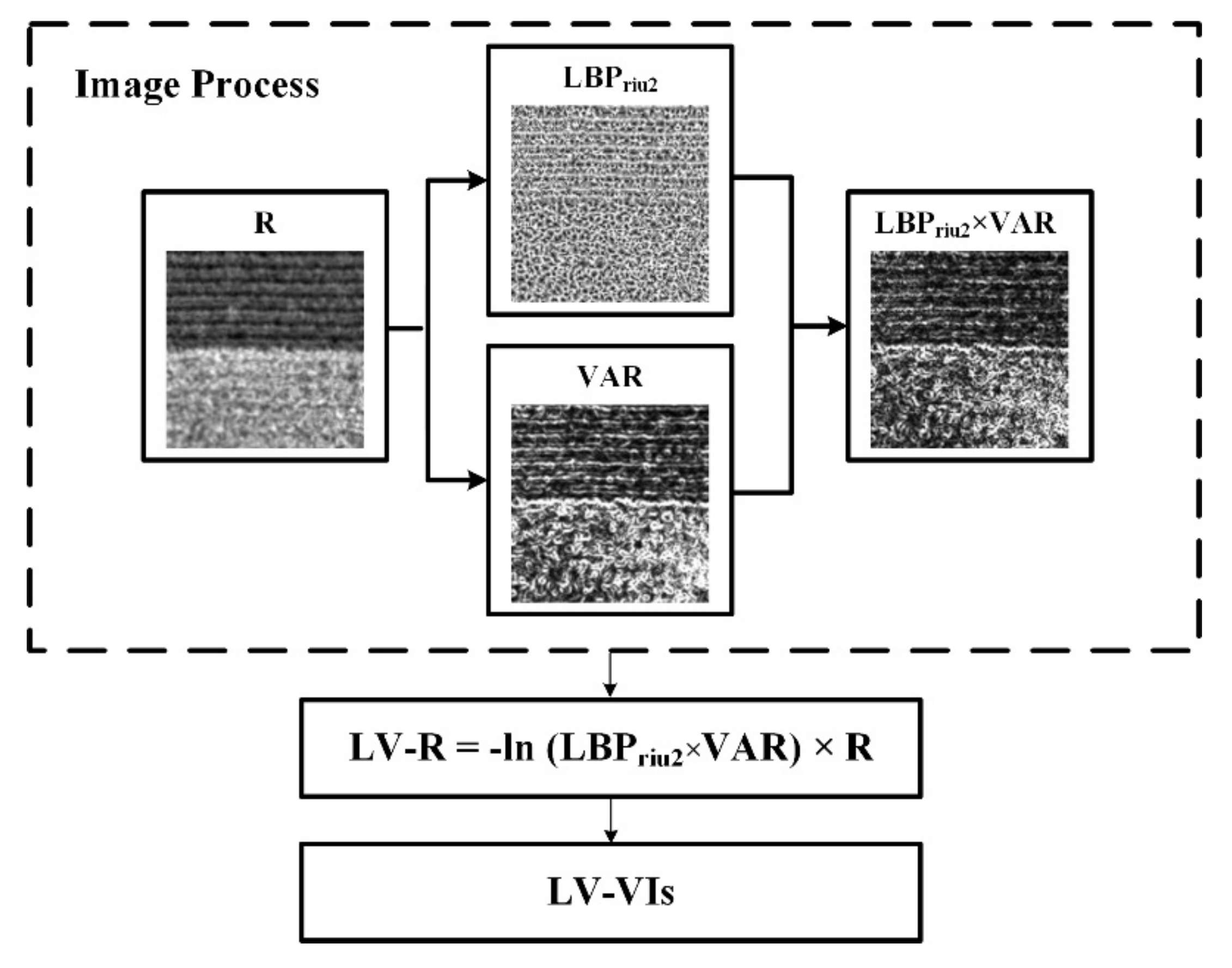
LBPriu2 and VAR were extracted from the reflectance images. To acquire a more comprehensive texture feature, the two texture images were multiplied pixel by pixel to obtain an LBP and VAR texture image, which was recorded as LBPriu2 × VAR. The plot-level LBPriu2 × VAR value was calculated by the average gray value of the pixels in ROI of LBPriu2 × VAR. To limit the influence of the panicles, the negative natural logarithm of LBPriu2 × VAR value was multiplied with the reflectance on the plot level, and the product was recorded as LV-R. Then the reflectance values in each VI formula were replaced with LV-Rs to obtain a new index, denoted as LV-VI (Figure 4). The calculated LV-VIs were evaluated for rice LAI estimation and were further compared with traditional VIs.

2.5. Algorithm Development for LAI Estimation

The final estimated model of LAI was developed by a k-fold cross-validation procedure. K-fold cross-validation was a statistical method which was widely applied in a model establishment [77,78,79]. In this study, k = 10, which is a common value used in many studies [77,79,80]. The samples were divided into k parts, k − 1 parts were applied to establish the model to obtain coefficients (Coefi) and coefficients of determination R i 2 , and the remaining part was regarded as the test set. The above steps were repeated k times, and the average values of root mean square error (RMSE) and coefficient of variation (CV) based on test set were calculated as follows [81]:
Coef = 1 k i = 1 k Coef i ; R 2 = 1 k i = 1 k R i 2 ;   RMSE = 1 k i = 1 k RMSE i ;   CV = 1 k i = 1 k CV i

3. Results

3.1. Relationships of VI vs. Rice LAI throughout the Entire Growing Season

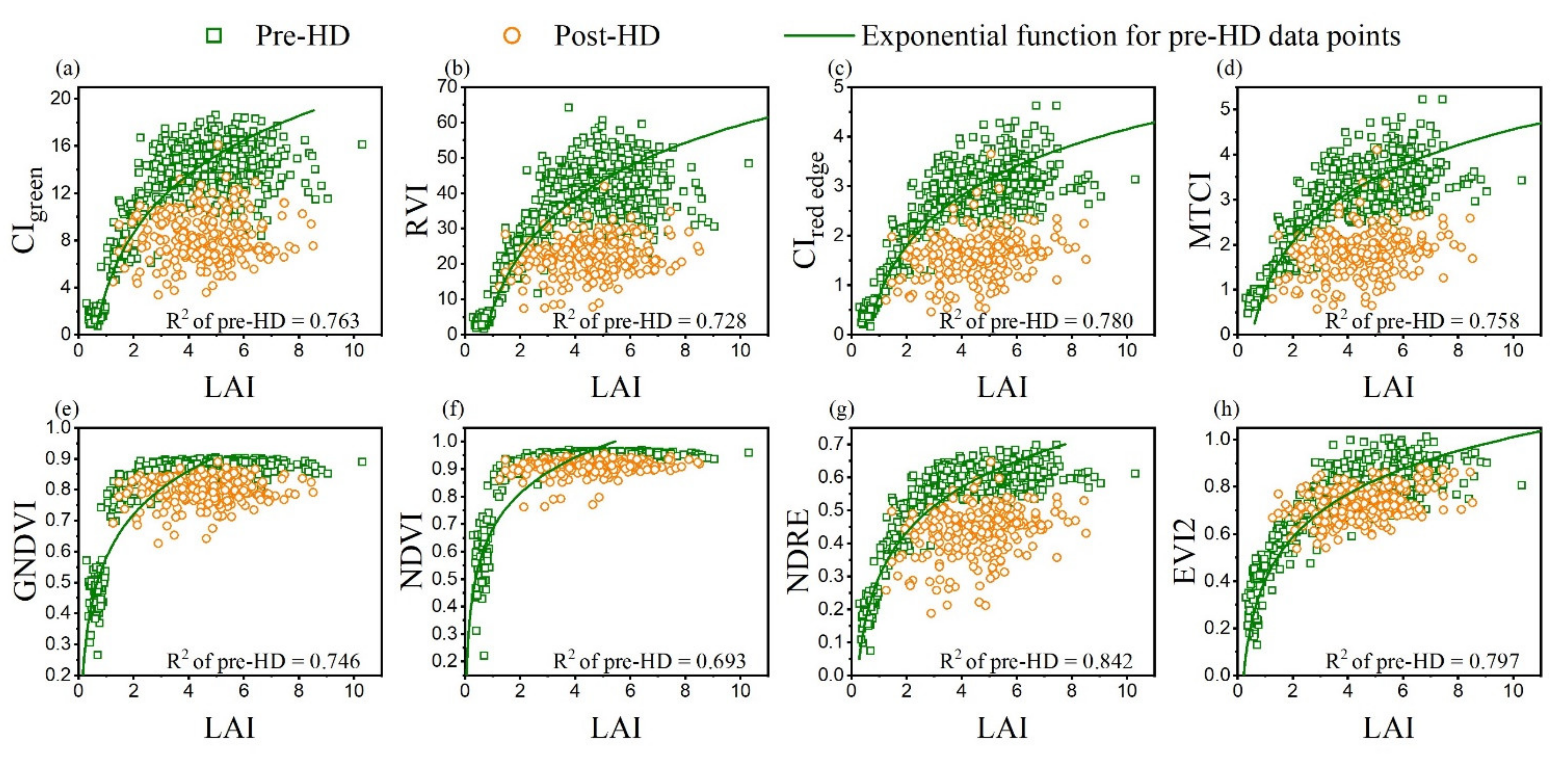
Some studies have proved that the exponential regression model is more suitable for fitting LAI and VI [34,37,82]. The R2 of the exponential regression model of ten VIs and the measured LAI throughout the entire growing season are shown in Table 4, of which MTCI was the lowest and EVI2 was the highest, though their scatter fitting results before heading were similar with R2 over 0.75 (Figure 5a,h). In addition, the R2 of ratio indices (CIred edge, CIgreen, and RVI) with similar scatter fitting results before heading were also generally low (R2 < 0.5), while the normalized indices (NDRE, GNDVI, and NDVI) were slightly higher (R2 > 0.5). The scattered points before heading and after heading of ratio indices and MTCI were more severely separated (Figure 5a–d), while those of normalized indices and EVI2 were slightly weaker (Figure 5e–h). The hysteresis effect could significantly decrease the R2 of LAI vs. VI fitting throughout the entire growing season.
As shown in Figure 5, all indices tended to reach saturation rapidly in moderate-to-high LAI variation before heading. The phenomenon of ratio indices was not as obvious as normalized indices. For normalized indices, the saturation of NDRE was not as obvious as GNDVI and NDVI. Comparing the R2 before heading, it is obvious that the saturation effect decreased the fitting accuracy of the pre-heading stage.

3.2. Rice LAI Estimation Combined with Texture Features

The changes of rice in different growth stages could be reflected by texture. At the vegetative stage, rice was planted in a stripe shape and the width of the stripe becomes wider as the rice grows [37]. When the leaves occluded most of the background, the wide stripes combined with each other to form a flat area covering the entire field. As the rice continued to grow, panicles began to emerge in the canopy, appearing as little dots in the image and breaking the flat texture. Therefore, the difference and complementarity of spectrum and texture in different growth stages could be utilized to assist VI in LAI estimation.

3.2.1. Variation of LBP and VAR in Pre-Heading Stages and Post-Heading Stages

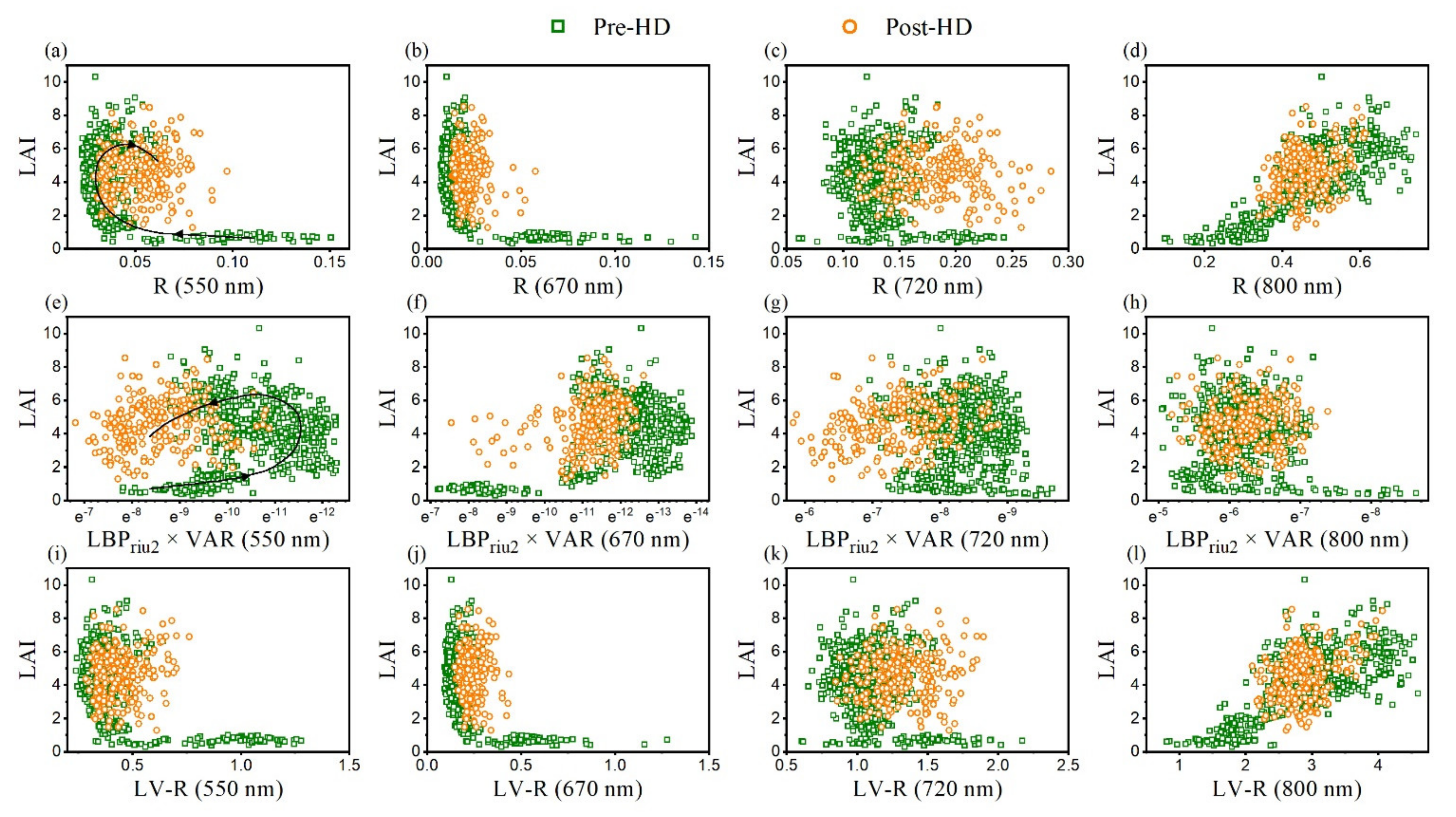
The relationships between LAI vs. plot-level reflectance (Figure 6a–d) and LAI vs. plot-level LBPriu2 × VAR (Figure 6e–h) are shown in Figure 6. Due to the difference in reflectivity and distribution of various objects shown in Figure 2, the results of texture varied in different wavebands (Figure 6e–h). The trends of time series changes of scatter distribution were opposite. In the scatter plot of LAI vs. reflectance, the time series bands of 550 nm, 670 nm, and 720 nm showed a counterclockwise distribution, while the same bands presented a clockwise distribution in LAI vs. LBPriu2 × VAR scatter plots. This made it possible to improve LAI estimation by combining the two indices. At the same time, with LAI increasing to a medium-high level before heading, the value of LBPriu2 × VAR was less saturated in the 550 nm and 670 nm bands, which made it beneficial for saturation reduction to combine the two indices. The relationships between the combined index LV-R and LAI are shown in Figure 6i–l. The hysteresis effects of LV-R at 550 nm, 670 nm, and 720 nm were obviously weakened, and the saturation effects at 550 nm and 670 nm were also slightly reduced.

3.2.2. Rice LAI Estimation Based on Remotely Sensed VI and LV-VI

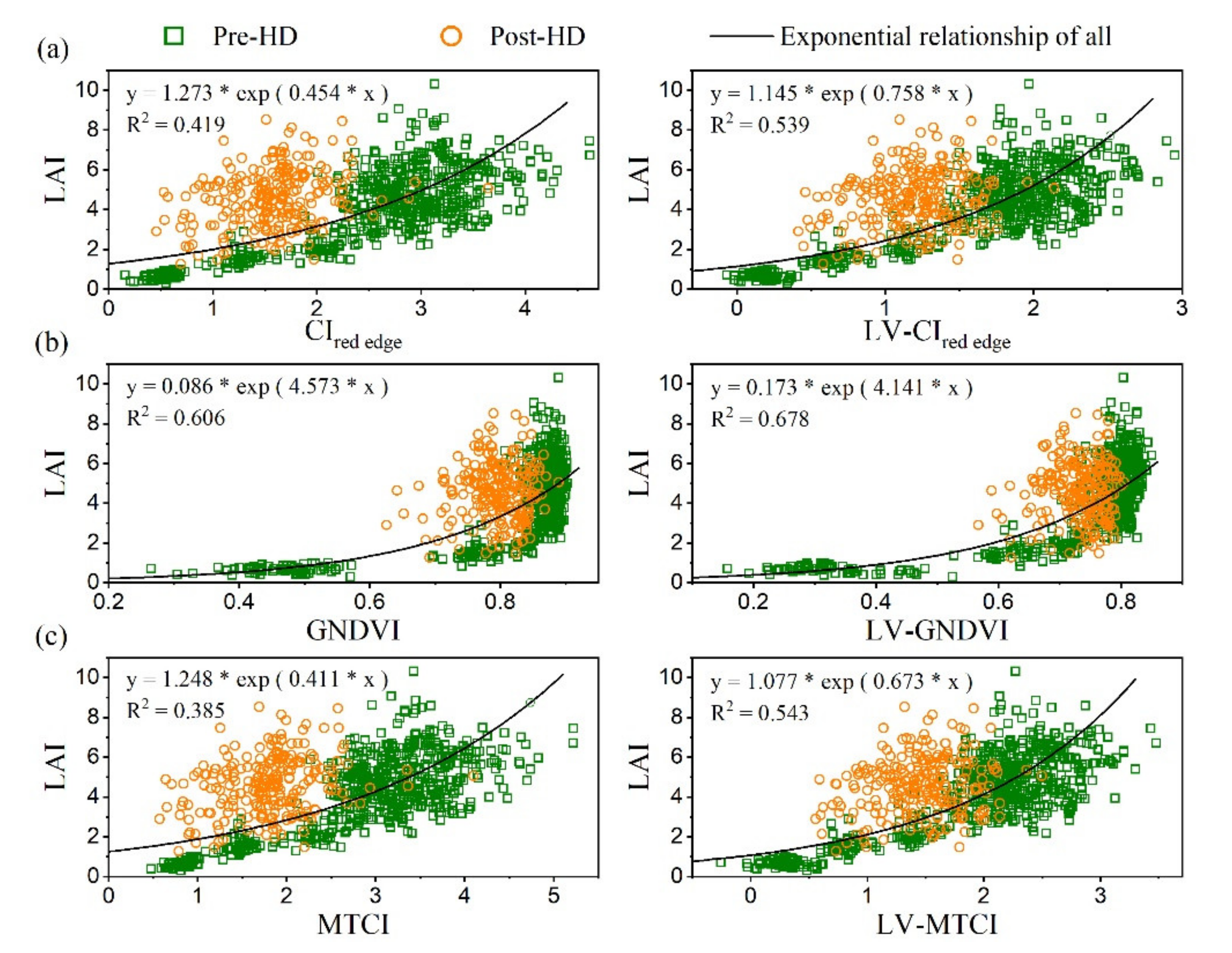
Figure 7 shows the comparable results of using textures to improve VIs. For all VIs, the scattered points after heading in LV-VIs were closer to the fitting curve of the whole growth stage than those in initial VIs, and the saturation effects before heading of all indices were also weakened. The saturation of the ratio indices was less obviously decreased than that of the normalized indices.
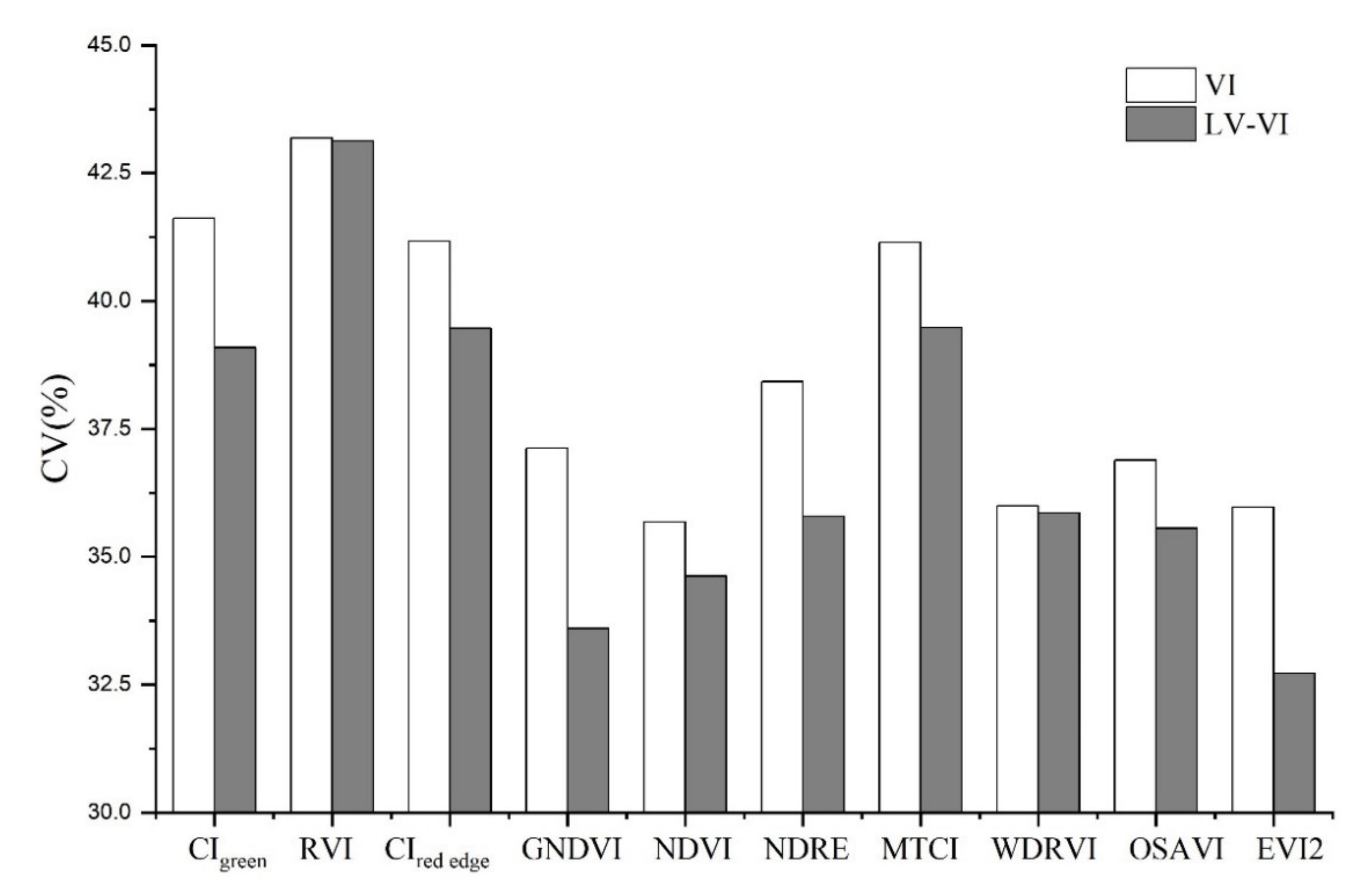
To verify the reliability of the model, R2 and RMSE statistics of VI and LV-VI after 10-fold cross-validation are shown in Table 5. All LV-VIs that combined with textures have improved the effect of using solely VIs to estimate LAI. Moreover, the improvement showed low dependence on the type of VIs used, including ratio, normalized, and modified indices. R2 increased by more than 0.13 (CIgreen, CIred edge, NDRE, and MTCI) and RMSE decreased by more than 0.1 (CIgreen, GNDVI, NDRE, EVI2). The inclusion of LBP and VAR features significantly improved the accuracy of the model for those containing the index of the 550 nm band (CIgreen and GNDVI), with CV decreased by more than 2.5%. There was also a notable improvement in the model containing the index of the 720 nm band (CIred edge, NDRE, MTCI, and OSAVI), with CV decreased more than 1.3% (Figure 8). However, for the model containing the index of the 670 nm band, the effect of accuracy improvement was uncertain. CV was decreased more than 3.2% for EVI2, while the improvements of others (RVI, WDRVI, and NDVI) were restricted.
The relationships between estimated LAI and measured LAI of some LV-VIs are shown in Figure 9. Considering the distribution and saturation of scattered points and values of R2 and RMSE, LV-CIgreen, LV-EVI2, and LV-NDRE were the best estimation models of rice LAI throughout the entire growing season in green, red, and red edge bands, respectively.

4. Discussion

In this study, we tested 10 commonly used VIs (CIgreen, RVI, CIred edge, GNDVI, NDVI, NDRE, MTCI, OSAVI, and EVI2) that had been widely applied in the estimation of LAI [19,78], biomass [61,83], and yield of crops [60,81]. When LAI reached a moderate-to-high variation, VIs were rapidly saturated, especially for the normalized VIs such as GNDVI, NDVI, and NDRE (Figure 5e–g). Considering only the period before heading, although these VIs were saturated with limited transitional zones, R2 could still reach above 0.65 (Figure 5). However, when the LAI of rice was estimated for the entire growing season, R2 was significantly reduced, and the decrease for MTCI was even more than 0.4 (Table 4).
The hysteresis effect after heading is a core issue that affects the accuracy of LAI estimation during the whole growing season of rice. Substantial hysteresis of the reflectance and canopy chlorophyll content had been discovered between the vegetative and reproductive stages in maize and soybean [84]. However, unlike the crops above, the hysteresis of rice was more exaggerated due to the complexity of the canopy structure. Rice leaves are more bent and crisscross with each other. The panicle is small and slender and varies with the growing period, so the complexity of the canopy increases [85,86]. The scattered points after heading in VI vs. LAI were clearly far away from those of the LAI vs. VI relationship before heading (Figure 5).
It is unrealistic, however, to establish a model before and after heading. The heading time of rice depends greatly on cultivars and environments, and recording the heading dates requires significant time and manpower, especially for breeding studies. Therefore, it is necessary to set an LAI estimation model for the entire growing season.
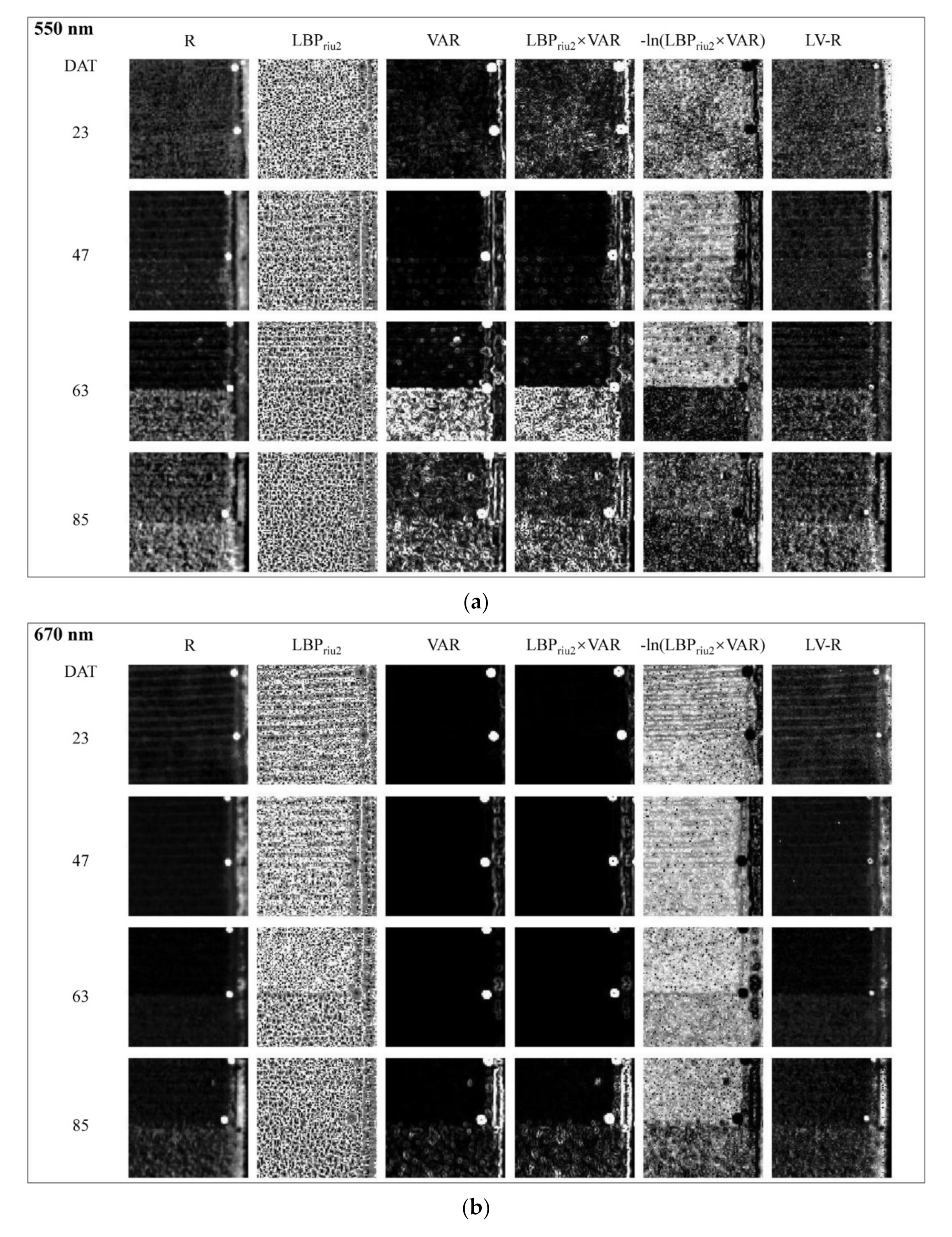
This study introduced the texture feature LBP and VAR to improve the VI model and to minimize the effect of saturation and hysteresis over the entire rice growing season. The spectral curves of typical features are very different before and after heading (Figure 2). Before heading, the field is mainly composed of leaves and soil background. Taking the tillering stage as an example, leaves are more reflective than soil in green bands due to the weak absorption of chlorophyll, while the reflectance of soil is slightly higher in the red and blue main absorption bands of chlorophyll [24]. As the rice grows, the soil background is gradually occluded by leaves and the appearance of panicles. At this time, only leaves and panicles are visible in the image. In the visible light band, panicles absorb less, mainly because they have a lower chlorophyll content than leaves [32]. In the NIR band, which is mainly affected by the structure of canopy, the area with the most panicles reflects more because of its higher canopy thickness [60]. Thus, in the pre-heading reflectance images in Figure 10 (DAT 23 and 47), the bright lines in the 550 nm, 720 nm, and 800 nm images are the leaves, while in 670 nm, the slightly bright lines are the soil background. In the post-heading reflectance images in Figure 10 (DAT 63 and 85), for the visible light bands such as 550 nm and 670 nm, the panicles are embedded in the leaves like stars. In the 720 nm and 800 nm reflectance images after heading, the bright lines represent the dense, thick canopies of panicles, and the dark lines are the thin canopies with leaves.
Based on the above analysis of the reflectivity and distribution of different objects, the texture extraction results of different bands are shown in Figure 10 (LBPriu2, VAR, LBP × VAR, −ln(LBP × VAR)).
The LBPriu2 and VAR of each individual pixel in the reflectance images were calculated separately, depicting local texture information (Figure 10). LBPriu2 only gave integer values between 0 and 9, as shown in Figure 3, which could distinguish bright spot features (with a value of 0), line or edge features (with values of 3–5), dark spot or flat features (with a value of 8), and so on. These features were related to the distribution of different objects in a rice field. As shown in Figure 10, in the first few days after transplanting (DAT 23), lines could be recognized in LBPriu2 images of any band due to the ridges in the field. As the rice grew, leaves gradually occluded soil background and continuous edges broke so that bright spots and flat areas increased simultaneously, and the entire brightness changed slightly and inconsistently. After rice heading, with panicles exerting, bright spots could be distinguished and the LBPriu2 image darkened (Figure 10). VAR calculated the variance of surrounding pixels and provided contrast information. Homogeneous areas have smaller values. As leaves gradually covered the background before heading, VAR values decreased and the image turned slightly darker. When panicles exserted after heading, these high reflected objects decreased the homogeneity and thus the brightness of the VAR images increased drastically (Figure 10). The edges of objects were usually fuzzy in VAR images, but these were much clearer under the specific values of LBPriu2.
The combination of LBPriu2 × VAR characteristics continued to follow the trend of VAR but showed more obvious differences between objects. In particular, the edges between leaves and soil background were thinned before heading, and the spots of panicles shrank after heading, both of which better represented the truth on the ground (Figure 10).
In terms of the image, the texture features of −ln(LBPriu2 × VAR) enhanced the differences in detail between the background and leaves before heading (Figure 10, DAT 23 and 47). At the same time, the gray values of the panicles in these images after heading were very low. In the LV-R image obtained by multiplying the texture image and the reflectance image, the influence of panicles was obviously suppressed (Figure 10, DAT 63 and 85) and thus LV-R indices were more suitable for constructing VIs throughout the entire growing season.
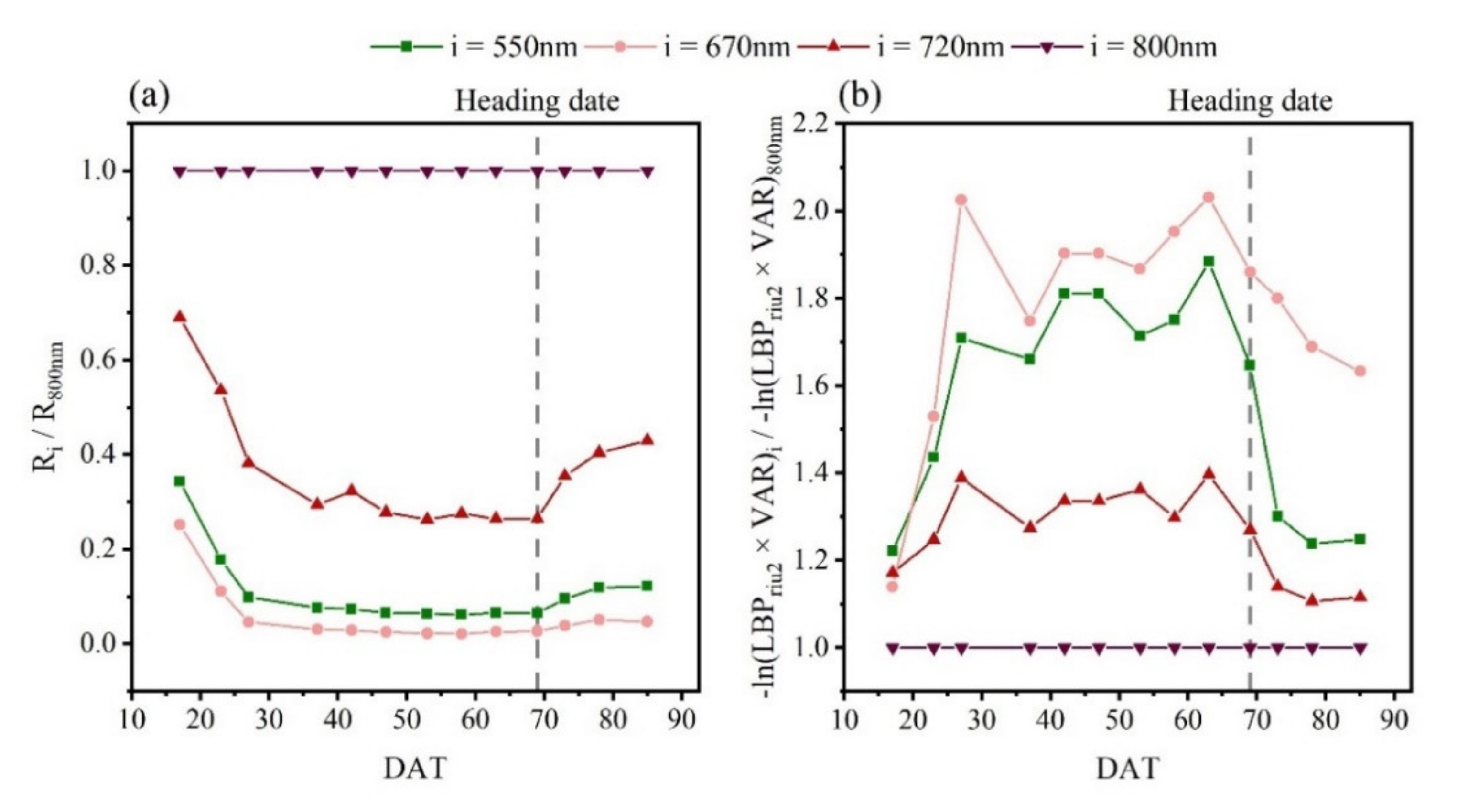
VIs presented the difference in reflectance between visible light and NIR [87]. In the tillering stage, this difference suddenly widened to a high level (Figure 11a), which led to saturation in VI vs. LAI (Figure 5). In contrast, the difference narrowed after heading (Figure 11a) which caused hysteresis (Figure 5). As a result of the time variation of LBPriu2 and VAR, the combination indices decreased slightly before heading and, remarkably, increased after heading in visible bands (Figure 10). Being unabsorbed by plants, VAR at 800 nm was not as sensitive to the variation of growth stages as those in visible bands (Figure 10), and so LBPriu2 × VAR with its negative logarithm changed less at 800 nm, meaning the difference between the visible and NIR bands narrowed after heading. As shown in Figure 11b, −ln(LBPriu2 × VAR) displayed the opposite trend to R. The relatively high value of logarithm index could narrow the difference in reflectance in the tillering stage, while the low value after heading could widen it and thus reduce the saturation and hysteresis effects. At the 670 nm band, however, −ln(LBPriu2 × VAR) had a relatively high value after heading and a weaker counterclockwise trend on the scatter plot with LAI (Figure 6). LV-VIs with dependence on indices at this band had less of an advantage than the others.
Comparing the LV-VI model with VI, as displayed in the scatter plot of Figure 7, reveals that the yellow part (after heading) data after processing are clearly similar to the green part (before heading) data. The slope of the turning point of the green part data also slowed down. By introducing texture features, the R2 of all tested VIs increased significantly, while RMSE and CV decreased significantly (Figure 8, Table 5). The method developed in our study is very simple for estimating rice LAI. It combines texture information with spectral information to effectively reduce saturation and hysteresis which emerges at certain stages. Compared with the physical model, the proposed model requires fewer parameters, thus avoiding the uncertainty of multiple rice cultivars and LAI estimation based on assumptions. The algorithms used in this study are exponential regressions that work rapidly and efficiently, meaning there was no need for sophisticated algorithms (e.g., machine learning method) requiring large-scale computation. This method only requires the use of reflectance images to estimate rice LAI during the entire growing season, and it is not necessary to establish a model before and after heading. Since VI, LBP, and VAR can be obtained by one UAV platform at a low cost, and can be simply and rapidly calculated from reflectance images, our method can be widely used in paddy field management and precision agriculture, especially in fields containing many cultivars for breeding.

5. Conclusions

In our study, we combined LBP and VAR with reflectance to construct new LV-VI parameters and applied them to LAI estimation. Compared with the corresponding VIs tested in this study, the fitting accuracy of all LV-VIs has been improved, R2 has been improved by up to 0.166 (MTCI), and RMSE and CV were 0.147 and 3.5% lower (GNDVI), respectively. The RMSE and CV of exponential fitting of LV-EVI2 were down to 1.367 and 32.7%, respectively. Considering the revealing effect of texture on different growth stages, LAI can be estimated more accurately by combining texture with spectrum. The combination of textural features enhances the contrast between crops and soil background in the image and weakens it between pixels with and without panicles. Moreover, it further adjusts the influence of reflectance given by the change of ground feature types in different growth stages. Therefore, in the LAI vs. VI scatters, the saturation before heading and the hysteresis effect after heading are obviously weakened. Since the LV-VI can be calculated simply and rapidly from a UAV reflectance image, our method provides a simple, low-cost option for crop growth monitoring and the progress of paddy field management, especially for rice breeding studies in fields containing a variety of cultivars. Future investigations are necessary to provide comparisons with different methods for estimating rice LAI, and to consider the underlying mechanisms of different textures throughout the entire growing season.

Author Contributions

All authors have made significant contributions to this manuscript. Y.G. and K.Y. designed the experiment and K.Y. performed the main experiments; B.D. and Y.P. gave important experimental guidance; K.Y. and N.Y. processed the data; S.F. and R.Z. provided the equipment and environment; X.W. and R.Z. offered advice based on agronomic perspectives; K.Y. and Y.G. wrote this manuscript together. All authors have read and agreed to the published version of the manuscript.

Funding

This research was supported by the advanced research project of civil space technology, National Natural Science Foundation of China (41771381), Key R & D projects in Hubei Province (2020BBB058), and National Key R&D Program of China (2016YFD0101105).

Institutional Review Board Statement

Not applicable.

Informed Consent Statement

Not applicable.

Acknowledgments

We thank the Lab for Remote Sensing of Crop Phenotyping Institute, School of Remote Sensing and Information Engineering, and College of Life Sciences, Wuhan University, China for providing the equipment and the use of the facilities. We are also grateful to the groups directed by Renshan Zhu and Shenghui Fang who worked hard in the field and in the lab to provide us with valuable data.

Conflicts of Interest

The authors declare that the research was conducted in the absence of any commercial or financial relationships that could be construed as a potential conflict of interest.

References

  1. Sesma, A.; Osbourn, A.E. The rice leaf blast pathogen undergoes developmental processes typical of root-infecting fungi. Nature 2004, 431, 582–586. [Google Scholar] [CrossRef]
  2. Yuan, L. Development of hybrid rice to ensure food security. Rice Sci. 2014, 21, 1–2. [Google Scholar] [CrossRef]
  3. Xu, X.Q.; Lu, J.S.; Zhang, N.; Yang, T.C.; He, J.Y.; Yao, X.; Cheng, T.; Zhu, Y.; Cao, W.X.; Tian, Y.C. Inversion of rice canopy chlorophyll content and leaf area index based on coupling of radiative transfer and Bayesian network models. ISPRS J. Photogramm. Remote Sens. 2019, 150, 185–196. [Google Scholar] [CrossRef]
  4. Watson, D.J. Comparative physiological studies on the growth of field crops: I. Variation in net assimilation rate and leaf area between species and varieties, and within and between years. Ann. Bot. 1947, 11, 41–76. [Google Scholar] [CrossRef]
  5. Yan, G.; Hu, R.; Luo, J.; Weiss, M.; Jiang, H.; Mu, X.; Xie, D.; Zhang, W. Review of indirect optical measurements of leaf area index: Recent advances, challenges, and perspectives. Agric. For. Meteorol. 2019, 265, 390–411. [Google Scholar] [CrossRef]
  6. Weiss, M.; Jacob, F.; Duveiller, G. Remote sensing for agricultural applications: A meta-review. Remote Sens. Environ. 2020, 236, 111402. [Google Scholar] [CrossRef]
  7. Goude, M.; Nilsson, U.; Holmström, E. Comparing direct and indirect leaf area measurements for Scots pine and Norway spruce plantations in Sweden. Eur. J. For. Res. 2019, 138, 1033–1047. [Google Scholar] [CrossRef] [Green Version]
  8. Qiao, K.; Zhu, W.; Xie, Z.; Li, P. Estimating the seasonal dynamics of the leaf area index using piecewise LAI-VI relationships based on phenophases. Remote Sens. 2019, 11, 689. [Google Scholar] [CrossRef] [Green Version]
  9. Liu, X.; Jin, J.; Herbert, S.J.; Zhang, Q.; Wang, G. Yield components, dry matter, LAI and LAD of soybeans in Northeast China. Field Crops Res. 2005, 93, 85–93. [Google Scholar] [CrossRef]
  10. Zhou, X.; Zheng, H.B.; Xu, X.Q.; He, J.Y.; Ge, X.K.; Yao, X.; Cheng, T.; Zhu, Y.; Cao, W.X.; Tian, Y.C. Predicting grain yield in rice using multi-temporal vegetation indices from UAV-based multispectral and digital imagery. ISPRS J. Photogramm. Remote Sens. 2017, 130, 246–255. [Google Scholar] [CrossRef]
  11. Fang, H.; Baret, F.; Plummer, S.; Schaepman-Strub, G. An overview of global leaf area index (LAI): Methods, products, validation, and applications. Rev. Geophys. 2019, 57, 739–799. [Google Scholar] [CrossRef]
  12. Asner, G.P.; Braswell, B.H.; Schimel, D.S.; Wessman, C.A. Ecological research needs from multiangle remote sensing data. Remote Sens. Environ. 1998, 63, 155–165. [Google Scholar] [CrossRef]
  13. Zheng, G.; Moskal, L.M. Retrieving leaf area index (LAI) using remote sensing: Theories, methods and sensors. Sensors 2009, 9, 2719–2745. [Google Scholar] [CrossRef] [Green Version]
  14. Boussetta, S.; Balsamo, G.; Beljaars, A.; Kral, T.; Jarlan, L. Impact of a satellite-derived leaf area index monthly climatology in a global numerical weather prediction model. Int. J. Remote Sens. 2012, 34, 3520–3542. [Google Scholar] [CrossRef]
  15. Breda, N.J. Ground-based measurements of leaf area index: A review of methods, instruments and current controversies. J. Exp. Bot. 2003, 54, 2403–2417. [Google Scholar] [CrossRef]
  16. Casanova, D.; Epema, G.F.; Goudriaan, J. Monitoring rice reflectance at field level for estimating biomass and LAI. Field Crops Res. 1998, 55, 83–92. [Google Scholar] [CrossRef]
  17. Yao, X.; Wang, N.; Liu, Y.; Cheng, T.; Tian, Y.; Chen, Q.; Zhu, Y. Estimation of wheat LAI at middle to high levels using unmanned aerial vehicle narrowband multispectral imagery. Remote Sens. 2017, 9, 7624. [Google Scholar] [CrossRef] [Green Version]
  18. Wang, L.; Chang, Q.; Yang, J.; Zhang, X.; Li, F. Estimation of paddy rice leaf area index using machine learning methods based on hyperspectral data from multi-year experiments. PLoS ONE 2018, 13, e0207624. [Google Scholar] [CrossRef] [PubMed] [Green Version]
  19. Dong, T.; Liu, J.; Shang, J.; Qian, B.; Ma, B.; Kovacs, J.M.; Walters, D.; Jiao, X.; Geng, X.; Shi, Y. Assessment of red-edge vegetation indices for crop leaf area index estimation. Remote Sens. Environ. 2019, 222, 133–143. [Google Scholar] [CrossRef]
  20. Darvishzadeh, R.; Skidmore, A.; Schlerf, M.; Atzberger, C. Inversion of a radiative transfer model for estimating vegetation LAI and chlorophyll in a heterogeneous grassland. Remote Sens. Environ. 2008, 112, 2592–2604. [Google Scholar] [CrossRef]
  21. Richter, K.; Atzberger, C.; Vuolo, F.; D’Urso, G. Evaluation of Sentinel-2 spectral sampling for radiative transfer model based LAI estimation of wheat, sugar beet, and maize. IEEE J. Sel. Top. Appl. Earth Obs. Remote Sens. 2011, 4, 458–464. [Google Scholar] [CrossRef]
  22. Atzberger, C.; Richter, K. Spatially constrained inversion of radiative transfer models for improved LAI mapping from future Sentinel-2 imagery. Remote Sens. Environ. 2012, 120, 208–218. [Google Scholar] [CrossRef]
  23. Campos-Taberner, M.; García-Haro, F.J.; Camps-Valls, G.; Grau-Muedra, G.; Nutini, F.; Crema, A.; Boschetti, M. Multitemporal and multiresolution leaf area index retrieval for operational local rice crop monitoring. Remote Sens. Environ. 2016, 187, 102–118. [Google Scholar] [CrossRef]
  24. Li, D.; Chen, J.M.; Zhang, X.; Yan, Y.; Zhu, J.; Zheng, H.; Zhou, K.; Yao, X.; Tian, Y.; Zhu, Y.; et al. Improved estimation of leaf chlorophyll content of row crops from canopy reflectance spectra through minimizing canopy structural effects and optimizing off-noon observation time. Remote Sens. Environ. 2020, 248, 111985. [Google Scholar] [CrossRef]
  25. Jay, S.; Maupas, F.; Bendoula, R.; Gorretta, N. Retrieving LAI, chlorophyll and nitrogen contents in sugar beet crops from multi-angular optical remote sensing: Comparison of vegetation indices and PROSAIL inversion for field phenotyping. Field Crops Res. 2017, 210, 33–46. [Google Scholar] [CrossRef] [Green Version]
  26. Liu, J.; Pattey, E.; Jégo, G. Assessment of vegetation indices for regional crop green LAI estimation from Landsat images over multiple growing seasons. Remote Sens. Environ. 2012, 123, 347–358. [Google Scholar] [CrossRef]
  27. Houborg, R.; Anderson, M.; Daughtry, C. Utility of an image-based canopy reflectance modeling tool for remote estimation of LAI and leaf chlorophyll content at the field scale. Remote Sens. Environ. 2009, 113, 259–274. [Google Scholar] [CrossRef]
  28. Rouse, J.W.; Haas, R.H.; Schell, J.A.; Deering, D.W. Monitoring vegetation systems in the great plains with ERTS. In NASA SP-351 Third ERTS-1 Symposium; Fraden, S.C., Marcanti, E.P., Becker, M.A., Eds.; Scientific and Technical Information Office, National Aeronautics and Space Administration: Washington, DC, USA, 1974; pp. 309–317. [Google Scholar]
  29. Viña, A.; Gitelson, A.A.; Nguy-Robertson, A.L.; Peng, Y. Comparison of different vegetation indices for the remote assessment of green leaf area index of crops. Remote Sens. Environ. 2011, 115, 3468–3478. [Google Scholar] [CrossRef]
  30. Yoshida, S. Fundamentals of Rice Crop Science; International Rice Research Institute: Los Baños, Philippines, 1981; pp. 1–61. [Google Scholar]
  31. Moldenhauer, K.; Counce, P.; Hardke, J. Rice Growth and Development. In Arkansas Rice Production Handbook; Hardke, J.T., Ed.; University of Arkansas Division of Agriculture Cooperative Extension Service: Little Rock, AR, USA, 2013; pp. 9–20. [Google Scholar]
  32. He, J.; Zhang, N.; Su, X.; Lu, J.; Yao, X.; Cheng, T.; Zhu, Y.; Cao, W.; Tian, Y. Estimating leaf area index with a new vegetation index considering the influence of rice panicles. Remote Sens. 2019, 11, 1809. [Google Scholar] [CrossRef] [Green Version]
  33. Sakamoto, T.; Shibayama, M.; Kimura, A.; Takada, E. Assessment of digital camera-derived vegetation indices in quantitative monitoring of seasonal rice growth. ISPRS J. Photogramm. Remote Sens. 2011, 66, 872–882. [Google Scholar] [CrossRef]
  34. Wang, Y.; Zhang, K.; Tang, C.; Cao, Q.; Tian, Y.; Zhu, Y.; Cao, W.; Liu, X. Estimation of rice growth parameters based on linear mixed-effect model using multispectral images from fixed-wing unmanned aerial vehicles. Remote Sens. 2019, 11, 1371. [Google Scholar] [CrossRef] [Green Version]
  35. Li, S.; Yuan, F.; Ata-Ui-Karim, S.T.; Zheng, H.; Cheng, T.; Liu, X.; Tian, Y.; Zhu, Y.; Cao, W.; Cao, Q. Combining color indices and textures of UAV-based digital imagery for rice lai estimation. Remote Sens. 2019, 11, 1793. [Google Scholar] [CrossRef] [Green Version]
  36. Ma, Y.; Jiang, Q.; Wu, X.; Zhu, R.; Gong, Y.; Peng, Y.; Duan, B.; Fang, S. Monitoring hybrid rice phenology at initial heading stage based on low-altitude remote sensing data. Remote Sens. 2020, 13, 86. [Google Scholar] [CrossRef]
  37. Duan, B.; Liu, Y.; Gong, Y.; Peng, Y.; Wu, X.; Zhu, R.; Fang, S. Remote estimation of rice LAI based on Fourier spectrum texture from UAV image. Plant Methods 2019, 15, 124. [Google Scholar] [CrossRef] [PubMed] [Green Version]
  38. Zhang, C.; Xie, Z. Combining object-based texture measures with a neural network for vegetation mapping in the Everglades from hyperspectral imagery. Remote Sens. Environ. 2012, 124, 310–320. [Google Scholar] [CrossRef]
  39. Lu, D. Aboveground biomass estimation using Landsat TM data in the Brazilian Amazon. Int. J. Remote Sens. 2007, 26, 2509–2525. [Google Scholar] [CrossRef]
  40. Zhou, J.; Guo, R.; Sun, M.; Di, T.T.; Wang, S.; Zhai, J.; Zhao, Z. The effects of GLCM parameters on LAI estimation using texture values from Quickbird satellite imagery. Sci. Rep. 2017, 7. [Google Scholar] [CrossRef] [PubMed]
  41. Ojala, T.; Pietikainen, M.; Harwood, D. A comparative study of texture measures with classification based on feature distributions. Pattern Recogn. 1996, 29, 51–59. [Google Scholar] [CrossRef]
  42. Song, X.; Chen, Y.; Feng, Z.; Hu, G.; Zhang, T.; Wu, X. Collaborative representation based face classification exploiting block weighted LBP and analysis dictionary learning. Pattern Recogn. 2019, 88, 127–138. [Google Scholar] [CrossRef]
  43. Liu, L.; Fieguth, P.; Guo, Y.; Wang, X.; Pietikäinen, M. Local binary features for texture classification: Taxonomy and experimental study. Pattern Recogn. 2017, 62, 135–160. [Google Scholar] [CrossRef] [Green Version]
  44. Heikkilä, M.; Pietikäinen, M.; Schmid, C. Description of interest regions with local binary patterns. Pattern Recogn. 2009, 42, 425–436. [Google Scholar] [CrossRef] [Green Version]
  45. Guo, Z.; Zhang, L.; Zhang, D. A completed modeling of local binary pattern operator for texture classification. IEEE Trans. Image Process. 2010, 19, 1657–1663. [Google Scholar] [CrossRef] [Green Version]
  46. Ji, L.; Ren, Y.; Liu, G.; Pu, X. Training-based gradient LBP feature models for multiresolution texture classification. IEEE Trans. Cybern. 2018, 48, 2683–2696. [Google Scholar] [CrossRef]
  47. Garg, M.; Dhiman, G. A novel content-based image retrieval approach for classification using GLCM features and texture fused LBP variants. Neural Comput. Appl. 2020. [Google Scholar] [CrossRef]
  48. Ma, Z.; Ding, Y.; Li, B.; Yuan, X. Deep CNNs with robust LBP guiding pooling for face recognition. Sensors 2018, 18, 3876. [Google Scholar] [CrossRef] [PubMed] [Green Version]
  49. Karanwal, S.; Diwakar, M. OD-LBP: Orthogonal difference-local binary pattern for face recognition. Digit. Signal Process. 2021, 110, 102948. [Google Scholar] [CrossRef]
  50. Nanni, L.; Lumini, A.; Brahnam, S. Local binary patterns variants as texture descriptors for medical image analysis. Artif. Intell. Med. 2010, 49, 117–125. [Google Scholar] [CrossRef]
  51. Yurdakul, O.C.; Subathra, M.S.P.; George, S.T. Detection of parkinson’s disease from gait using neighborhood representation local binary patterns. Biomed. Signal Process. 2020, 62, 102070. [Google Scholar] [CrossRef]
  52. Yazid, M.; Abdur Rahman, M. Variable step dynamic threshold local binary pattern for classification of atrial fibrillation. Artif. Intell. Med. 2020, 108, 101932. [Google Scholar] [CrossRef]
  53. Vilbig, J.M.; Sagan, V.; Bodine, C. Archaeological surveying with airborne LiDAR and UAV photogrammetry: A comparative analysis at Cahokia Mounds. J. Archaeol. Sci. Rep. 2020, 33, 102509. [Google Scholar] [CrossRef]
  54. Hamouchene, I.; Aouat, S.; Lacheheb, H. Texture Segmentation and Matching Using LBP Operator and GLCM Matrix. In Intelligent Systems for Science and Information. Studies in Computational Intelligence; Chen, L., Kapoor, S., Bhatia, R., Eds.; Springer: Cham, Switzerland, 2014; Volume 542. [Google Scholar]
  55. Peuna, A.; Thevenot, J.; Saarakkala, S.; Nieminen, M.T.; Lammentausta, E. Machine learning classification on texture analyzed T2 maps of osteoarthritic cartilage: Oulu knee osteoarthritis study. Osteoarthr. Cartil. 2021, 29, 859–869. [Google Scholar] [CrossRef]
  56. Ojala, T.; Pietikäinen, M.; Mäenpää, T. Gray Scale and Rotation Invariant Texture Classification with Local Binary Patterns. In Proceedings of the 6th European Conference on Computer Vision, Dublin, Ireland, 26 June–1 July 2000; pp. 404–420. [Google Scholar]
  57. Guo, Z.; Zhang, L.; Zhang, D. Rotation invariant texture classification using LBP variance (LBPV) with global matching. Pattern Recogn. 2010, 43, 706–719. [Google Scholar] [CrossRef]
  58. Wang, F.-m.; Huang, J.-f.; Tang, Y.-l.; Wang, X.-z. New vegetation index and its application in estimating leaf area index of rice. Rice Sci. 2007, 14, 195–203. [Google Scholar] [CrossRef]
  59. Jiang, Q.; Fang, S.; Peng, Y.; Gong, Y.; Zhu, R.; Wu, X.; Ma, Y.; Duan, B.; Liu, J. UAV-based biomass estimation for rice-combining spectral, Tin-based structural and meteorological features. Remote Sens. 2019, 11, 890. [Google Scholar] [CrossRef] [Green Version]
  60. Duan, B.; Fang, S.; Zhu, R.; Wu, X.; Wang, S.; Gong, Y.; Peng, Y. Remote estimation of rice yield with unmanned aerial vehicle (UAV) data and spectral mixture analysis. Front. Plant Sci. 2019, 10, 204. [Google Scholar] [CrossRef] [Green Version]
  61. Zheng, H.; Cheng, T.; Zhou, M.; Li, D.; Yao, X.; Tian, Y.; Cao, W.; Zhu, Y. Improved estimation of rice aboveground biomass combining textural and spectral analysis of UAV imagery. Precis. Agric. 2018, 20, 611–629. [Google Scholar] [CrossRef]
  62. Yuan, N.; Gong, Y.; Fang, S.; Liu, Y.; Duan, B.; Yang, K.; Wu, X.; Zhu, R. UAV remote sensing estimation of rice yield based on adaptive spectral endmembers and bilinear mixing model. Remote Sens. 2021, 13, 2190. [Google Scholar] [CrossRef]
  63. Zheng, H.; Cheng, T.; Li, D.; Yao, X.; Tian, Y.; Cao, W.; Zhu, Y. Combining unmanned aerial vehicle (UAV)-based multispectral imagery and ground-based hyperspectral data for plant nitrogen concentration estimation in rice. Front. Plant Sci. 2018, 9, 936. [Google Scholar] [CrossRef] [PubMed]
  64. Smith, G.M.; Milton, E.J. The use of the empirical line method to calibrate remotely sensed data to reflectance. Int. J. Remote Sens. 2010, 20, 2653–2662. [Google Scholar] [CrossRef]
  65. Laliberte, A.S.; Goforth, M.A.; Steele, C.M.; Rango, A. Multispectral Remote Sensing from Unmanned Aircraft: Image Processing Workflows and Applications for Rangeland Environments. Remote Sens. 2011, 3, 2529–2551. [Google Scholar] [CrossRef] [Green Version]
  66. Baugh, W.M.; Groeneveld, D.P. Empirical proof of the empirical line. Int. J. Remote Sens. 2007, 29, 665–672. [Google Scholar] [CrossRef]
  67. Gitelson, A.A.; Gritz, Y.; Merzlyak, M.N. Relationships between leaf chlorophyll content and spectral reflectance and algorithms for non-destructive chlorophyll assessment in higher plant leaves. J. Plant Physiol. 2003, 160, 271–282. [Google Scholar] [CrossRef] [PubMed]
  68. Gitelson, A.A.; Kaufman, Y.J.; Merzlyak, M.N. Use of a green channel in remote sensing of global vegetation from EOS-MODIS. Remote Sens. Environ. 1996, 58, 289–298. [Google Scholar] [CrossRef]
  69. Rouse, J.W.; Haas, R.H.; Schell, J.A.; Deering, D.W. Monitoring the Vernal Advancement and Retrogradation (Greenwave Effect) of Natural Vegetation; NASA/GSFC Type III Final Report; NASA/GSFC: Greenbelt, MD, USA, 1974. [Google Scholar]
  70. Fitzgerald, G.; Rodriguez, D.; O’Leary, G. Measuring and predicting canopy nitrogen nutrition in wheat using a spectral index—The canopy chlorophyll content index (CCCI). Field Crops Res. 2010, 116, 318–324. [Google Scholar] [CrossRef]
  71. Dash, J.; Curran, P.J. The MERIS terrestrial chlorophyll index. Int. J. Remote Sens. 2004, 25, 5403–5413. [Google Scholar] [CrossRef]
  72. Gitelson, A.A. Wide dynamic range vegetation index for remote quantification of biophysical characteristics of vegetation. J. Plant Physiol. 2004, 161, 165–173. [Google Scholar] [CrossRef] [Green Version]
  73. Rondeaux, G.; Steven, M.; Baret, F. Optimization of soil-adjusted vegetation indices. Remote Sens. Environ. 1996, 55, 95–107. [Google Scholar] [CrossRef]
  74. Jiang, Z.; Huete, A.; Didan, K.; Miura, T. Development of a two-band enhanced vegetation index without a blue band. Remote Sens. Environ. 2008, 112, 3833–3845. [Google Scholar] [CrossRef]
  75. Wang, A.; Wang, S.; Lucieer, A. Segmentation of multispectral high-resolution satellite imagery based on integrated feature distributions. Int. J. Remote Sens. 2010, 31, 1471–1483. [Google Scholar] [CrossRef]
  76. Lucieer, A.; Stein, A.; Fisher, P. Multivariate texture-based segmentation of remotely sensed imagery for extraction of objects and their uncertainty. Int. J. Remote Sens. 2005, 26, 2917–2936. [Google Scholar] [CrossRef]
  77. Kohavi, R. A Study of Cross-Validation and Bootstrap for Accuracy Estimation and Model Selection. In Proceedings of the International Joint Conference on Articial Intelligence, Montreal, QC, Canada, 20–25 August 1995; pp. 1137–1145. [Google Scholar]
  78. Nguy-Robertson, A.; Gitelson, A.; Peng, Y.; Viña, A.; Arkebauer, T.; Rundquist, D. Green leaf area index estimation in maize and soybean: Combining vegetation indices to achieve maximal sensitivity. Agron. J. 2012, 104, 1336–1347. [Google Scholar] [CrossRef] [Green Version]
  79. Kira, O.; Nguy-Robertson, A.L.; Arkebauer, T.J.; Linker, R.; Gitelson, A.A. Toward generic models for green LAI estimation in maize and soybean: Satellite observations. Remote Sens. 2017, 9, 318. [Google Scholar] [CrossRef] [Green Version]
  80. Asrola, M.; Papilob, P.; Gunawan, F.E. Support Vector Machine with K-fold Validation to Improve the Industry’s Sustainability Performance Classification. Procedia Comput. Sci. 2021, 179, 854–862. [Google Scholar] [CrossRef]
  81. Peng, Y.; Zhu, T.; Li, Y.; Dai, C.; Fang, S.; Gong, Y.; Wu, X.; Zhu, R.; Liu, K. Remote prediction of yield based on LAI estimation in oilseed rape under different planting methods and nitrogen fertilizer applications. Agric. For. Meteorol. 2019, 271, 116–125. [Google Scholar] [CrossRef]
  82. Baret, F.; Guyot, G. Potentials and limits of vegetation indices for LAI and APAR assessment. Remote Sens. Environ. 1991, 35, 161–173. [Google Scholar] [CrossRef]
  83. Yue, J.; Yang, G.; Tian, Q.; Feng, H.; Xu, K.; Zhou, C. Estimate of winter-wheat above-ground biomass based on UAV ultrahighground-resolution image textures and vegetation indices. ISPRS J. Photogramm. Remote Sens. 2019, 150, 226–244. [Google Scholar] [CrossRef]
  84. Peng, Y.; Nguy-Robertson, A.; Arkebauer, T.; Gitelson, A. Assessment of canopy chlorophyll content retrieval in maize and soybean: Implications of hysteresis on the development of generic algorithms. Remote Sens. 2017, 9, 226. [Google Scholar] [CrossRef] [Green Version]
  85. Reza, M.N.; Na, I.S.; Baek, S.W.; Lee, K.-H. Rice yield estimation based on K-means clustering with graph-cut segmentation using low-altitude UAV images. Biosyst. Eng. 2019, 177, 109–121. [Google Scholar] [CrossRef]
  86. Zha, H.; Miao, Y.; Wang, T.; Li, Y.; Zhang, J.; Sun, W.; Feng, Z.; Kusnierek, K. Improving unmanned aerial vehicle remote sensing-based rice nitrogen nutrition index prediction with machine learning. Remote Sens. 2020, 12, 215. [Google Scholar] [CrossRef] [Green Version]
  87. Bannari, A.; Morin, D.; Bonn, F.; Huete, A.R. A review of vegetation indices. Remote Sens. Rev. 1995, 13, 95–120. [Google Scholar] [CrossRef]
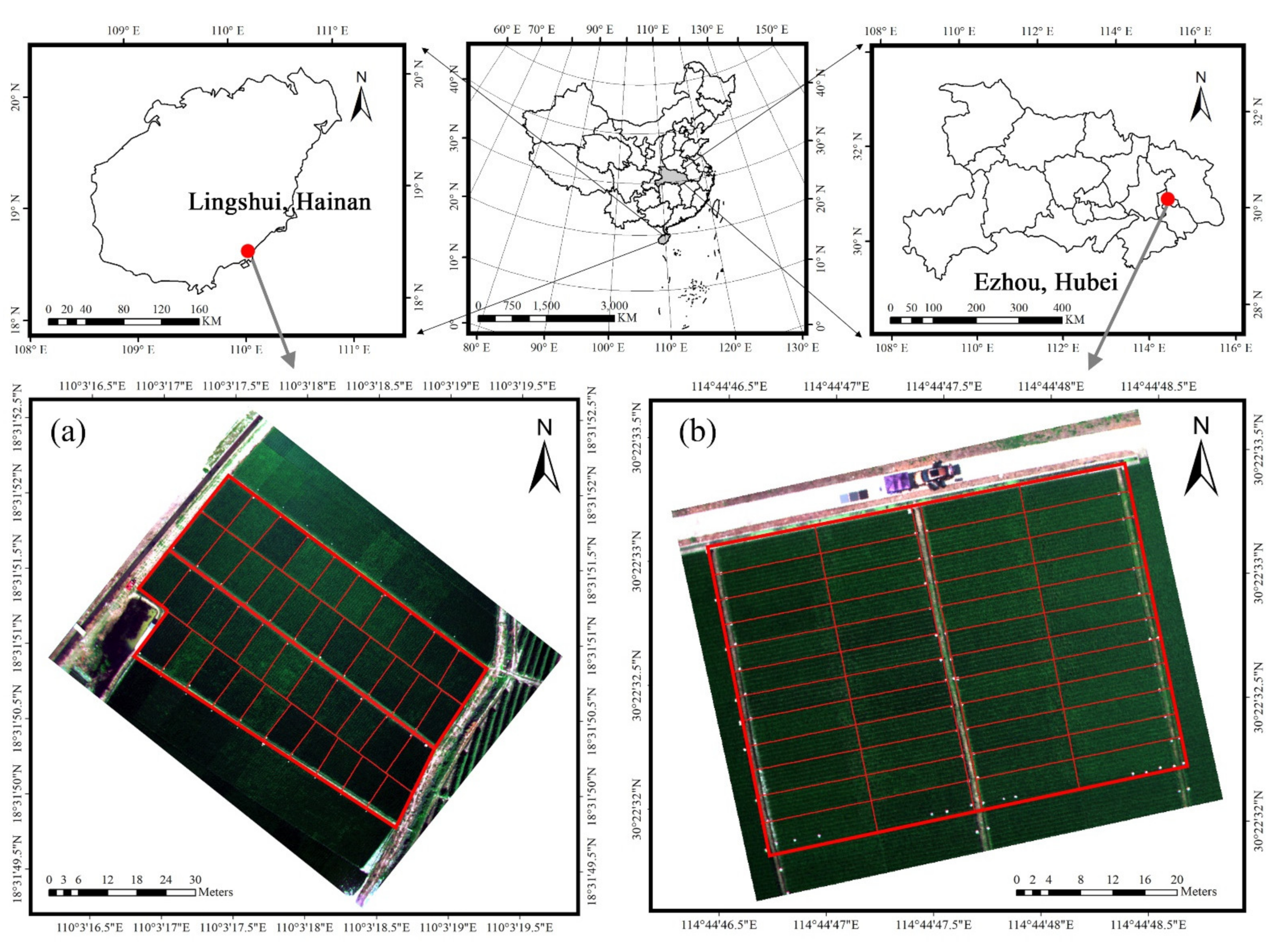
Figure 1. Study Area. (a) is the study area of Experiment 1 conducted in Hainan in 2018. (b) is the study area of Experiment 2 conducted in Hubei in 2019.
Remotesensing 13 03001 g001
Figure 2. Reflectance variation of different objects extracted on the reflectance image. (a) is the reflectance of leaf and soil before heading. (b) is the reflectance of leaf and panicle after heading.
Remotesensing 13 03001 g002
Figure 3. LBP patterns representing local features of spot, line, edge, and flat.
Remotesensing 13 03001 g003
Figure 4. Image processing for calculating LV-VIs. R represents reflectance.
Remotesensing 13 03001 g004
Figure 5. The variation of LAI plotted against vegetation indices: (a) CIgreen, (b) RVI, (c) CIred edge, (d) MTCI, (e) GNDVI, (f) NDVI, (g) NDRE and (h) EVI2 during the entire growing season. Pre-HD and Post-HD denote pre-heading stages and post-heading stages, respectively. For all tested indices, the samples after heading were deviated from the LAI vs. VI relationship before heading.
Remotesensing 13 03001 g005
Figure 6. Rice LAI plotted against the reflectance of (a) 550 nm, (b) 670 nm, (c) 720 nm, (d) 800 nm, the LBPriu2 × VAR calculated based on the bands of (e) 550 nm, (f) 670 nm, (g) 720 nm, (h) 800 nm, and the LV-R of (i) 550 nm, (j) 670 nm, (k) 720 nm, (l) 800 nm during the entire growth season. When the horizontal axis of LBPriu2 × VAR was expressed in exponential form, it was the opposite of the trend of LAI vs. reflectance. The LV-R index combining R and LBPriu2 × VAR had a smaller separation than R between pre-heading stages (Pre-HD) and post-heading stages (Post-HD).
Remotesensing 13 03001 g006
Figure 7. Two models of VI and LV-VI were tested for rice LAI estimation throughout the entire growing season on (a) CIred edge, (b) GNDVI, and (c) MTCI.
Remotesensing 13 03001 g007
Figure 8. The coefficients of variance (CV) for LAI estimation using VI and LV-VI, respectively.
Remotesensing 13 03001 g008
Figure 9. The relationship between Estimated LAI and Measured LAI based on (a) LV-CIgreen, (b) LV-EVI2, and (c) LV-NDRE.
Remotesensing 13 03001 g009
Figure 10. Image reflectance and texture changes of two plots at (a) 550 nm, (b) 670 nm, (c) 720 nm, and (d) 800 nm on the 23rd, 47th, 63rd, and 85th days after transplanting (DAT). R represents reflectance image. LBPriu2, VAR, LBPriu2 × VAR, −ln(LBPriu2 × VAR), and LV-R represent the corresponding images calculated by these methods.
Remotesensing 13 03001 g010aRemotesensing 13 03001 g010b
Figure 11. Temporal behaviors of (a) the reflectance ratio of visible and NIR and (b) the −ln(LBPriu2 × VAR) ratio of visible and NIR during the entire rice growing season. −ln(LBPriu2 × VAR) showed the opposite trend to R. The relatively high value of the logarithm index could narrow the difference of reflectance in the tillering stage, while the low value after heading could widen it instead, thus reducing the saturation and hysteresis effects.
Remotesensing 13 03001 g011
Table 1. Data acquisition time, date of transplanting (DAT), and corresponding growth stages of two experiments.
Growth StageExperiment 1: HainanExperiment 2: Ezhou
UAV ImagesLAI SamplingDATUAV ImagesLAI SamplingDAT
Tillering---26 June 201926 June 201917
---2 July 20192 July 201923
2 February 20184 February 2018276 July 20196 July 201927
---14 July 201916 July 201937
---22 July 201921 July 201942
26 February 201825 February 20184827 July 201926 July 201947
Jointing---1 August 20191 August 201953
11 March 20189 March 2018606 August 20196 August 201958
Booting and heading---11 August 201911 August 201963
18 March 201819 March 20187016 August 201917 August 201969
Ripening---22 August 201921 August 201973
---29 August 201926 August 201978
1 April 201831 March 2018823 September 20192 September 201985
15 April 201817 April 201899---
Note: ‘-’ means lack of data corresponding to the other experiment.
Table 2. Center wavelength and band width of each spectral band of the customized 12-lens Mini-MCA camera.
Center Wavelength (nm) Band Width(nm)Center Wavelength (nm)Band Width (nm)
490 10 700 10
520 10 720 10
550 10 800 10
570 10 850 10
670 10 900 20
680 10 950 40
Table 3. The vegetation indices that were tested in the study.
VIFormulaReference
Ratio
Indices
Green Chlorophyll Index (CIgreen) R 800 nm / R 550 nm 1 [67]
Ratio Vegetation Index (RVI) R 800 nm / R 670 nm [28]
Red-edge Chlorophyll Index (CIred edge) R 800 nm / R 720 nm 1 [67]
Normalized IndicesGreen Normalized Difference Vegetation Index (GNDVI) ( R 800 nm R 550 nm ) / ( R 800 nm + R 550 nm ) [68]
Normalized Difference Vegetation Index (NDVI) ( R 800 nm R 670 nm ) / ( R 800 nm + R 670 nm ) [69]
Normalized Difference Red-edge Vegetation Index (NDRE) ( R 800 nm R 720 nm ) / ( R 800 nm + R 720 nm ) [70]
Modified
Indices
MERIS Terrestrial Chlorophyll Index (MTCI) ( R 800 nm R 720 nm ) / ( R 720 nm R 670 nm ) [71]
Wide Dynamic Range Vegetation Index (WDRVI) ( α × R 800 nm R 670 nm ) / ( α × R 800 nm + R 670 nm ) , α = 0.2 [72]
Optimized Soil-Adjusted Vegetation Index (OSAVI)(1+0.16) × ( R 800 nm R 720 nm ) / ( R 800 nm + R 720 nm + 0.16 ) [73]
Two-band Enhanced Vegetation Index (EVI2) 2.5 × ( R 800 nm R 670 nm ) / ( 1 + R 800 nm + 2.4 × R 670 nm ) [74]
Table 4. Exponential regression of rice LAI with VIs during the entire growing season.
VIMTCICIred edgeCIgreenRVINDREOSAVIGNDVINDVIWDRVIEVI2
R20.3850.4190.4260.430.5250.580.6060.6180.6450.704
Table 5. Performance of the VI and LV-VI models based on 10-fold cross-validation.
VILV-VI
R2RMSER2RMSE
CIgreen0.400 1.738 0.552 1.633
RVI0.368 1.804 0.422 1.802
CIred edge0.394 1.720 0.527 1.648
GNDVI0.592 1.551 0.644 1.403
NDVI0.574 1.490 0.633 1.446
NDRE0.485 1.605 0.617 1.495
MTCI0.373 1.719 0.539 1.649
WDRVI0.608 1.504 0.643 1.498
OSAVI0.553 1.541 0.631 1.485
EVI20.675 1.503 0.719 1.367
Publisher’s Note: MDPI stays neutral with regard to jurisdictional claims in published maps and institutional affiliations.