A Novel Modeling Strategy of Weighted Mean Temperature in China Using RNN and LSTM

Abstract

In the meteorology of Global Navigation Satellite System, the weighted mean temperature (Tm) is a key parameter in the process of converting the zenith wetness delay into precipitable water vapor, and it plays an important role in water vapor monitoring. In this research, two deep learning algorithms, namely, recurrent neural network (RNN) and long short-term memory neural network (LSTM), were used to build a high-precision weighted mean temperature model for China using their excellent time series memory capability. The model needs site location information and measured surface temperature to predict the weighted mean temperature. We used data from 118 stations in and around China provided by the Integrated Global Radiosonde Archive from 2010 to 2015 to train the model and data from 2016 for model testing. The root mean square error (RMSE) of the RNN_Tm and LSTM_Tm models were 3.01 K and 2.89 K, respectively. Compared with the values calculated by the empirical GPT3 model, the accuracy was improved by 31.1% (RNN_Tm) and 33.9% (LSTM_Tm). In addition, we selected another 10 evenly distributed stations in China and used the constructed model to test the prediction capability of the weighted mean temperature from 2010 to 2016. The RMSE values were 2.95 K and 2.86 K, which proved that the model also exhibits high generalization in non-modeling sites in China. In general, the RNN_Tm and LSTM_Tm models have a good performance in weighted mean temperature prediction.

1. Introduction

The water vapor in the earth’s atmosphere is mainly concentrated in the troposphere, which plays an important role in climate change and energy transmission. Compared with traditionally used water vapor radiometers, radiosondes, and other methods, global navigation and positioning systems have numerous advantages, such as low cost and high temporal and spatial resolution, in water vapor detection applications. The weighted mean temperature is an important branch of Global Navigation Satellite System (GNSS) meteorology. This parameter is important for the conversion of tropospheric zenith wetness delay into precipitable water vapor (PWV). The concept of Tm was first proposed in [1]. In [2], the use of GPS to invert PWV was proposed, and the relationship between PWV, ZWD, and Tm was derived. Therefore, obtaining high-precision Tm data is important for GNSS water vapor inversion. The most accurate Tm value is obtained by using a radiosonde to acquire the atmospheric profile, measure meteorological parameters accurately, and integrate the temperature and water vapor pressure profile values in the vertical direction. However, this method is costly, and obtaining Tm data at any position is difficult. The model method is currently the primary way of obtaining Tm. The first kind of model is based on the measured meteorological parameters, and it is usually constructed by analyzing the relationship between meteorological data and the Tm value. In [3], 13 radiosonde stations distributed in the United States were used to fit the liner relationship between Tm and Ts to construct a Tm prediction model called Bevis Tm model (BTm), and the root mean square error (RMSE) was about 4.7 K. The BTm model is widely used; however, given that this model is constructed using U.S. sounding data, its accuracy in other regions is limited. In [4], the linear relationship between Tm and Ts was also used, but the latitude was divided into 12 regions; the coefficient values were calculated, and the global Tm model (GTm) was constructed. Through this modeling idea, numerous scholars have constructed the precise Tm model of the region; in [5], the data of 109 sounding stations in the European region were used to construct a Tm model suitable for Europe. The second kind model is empirical model with no meteorological parameters. These models can obtain an estimated value of Tm without the input of meteorological parameters. In [6,7,8], global weighted mean temperature (GWMT), global Tm model II (GTm-II), and global Tm model III (GTm-III) models were constructed. In [9,10], the global pressure and temperature 2w (GPT_2W) and global pressure and temperature 3 (GPT3) models, which can provide high-precision Tm experience value through grid data, were constructed. The Gtrop model was constructed in [11], which proposed an empirical model covering the ground surface to an altitude of 10 km. In addition, various empirical models of Tm have been established [12,13,14,15,16,17,18].

The above models are used by the majority of users due to their ease of use. However, regardless of whether there is the input of meteorological parameters, the accuracy of these two types of models is limited. The development of machine learning algorithms has greatly promoted the development of various fields. Such algorithms have excellent capability to fit complex nonlinear relationships. With the accumulation of more meteorological data sets, a Tm model can be possibly built with machine learning methods. In [19], they used the back propagation neural network (BPNN) to establish the first application of machine learning to Tm modeling and constructed the NN model to estimate the Tm value; the RMSE of the model was 3.3 K. In [20], the NN-II model was built on the basis of NN model; thus, the estimated Tm data covered the surface to the top of troposphere. In [21], an improved atmospheric Tm modeling method that uses sparse kernel learning to obtain high-precision and high-time resolution Tm data was proposed. In [22] random forest, BPNN, and generalized regression BPNN network to apply Tm modeling and obtain high-precision Tm estimates was used.

Machine learning algorithm has excellent modeling ability, so it also has many applications in hydrology and estimating climate parameters, such as soil moisture, wind speed, temperature, precipitation, water flow and so on. In [23], support vector machine (SVM) method is used to predict soil moisture. In [24], the extreme learning machine is applied to the prediction of wind speed to fit the relationship between wind speeds at different heights. In [25], two methods of random forest and neural network are used to construct an improved IMERG precipitation product. In [26], enhanced extreme learning machine is used to predict water flow. In [27], quantile regression and parameter regression technique are used for flood frequency analysis. In [28], 511 GR4J hydrological models in the United States were post-processing simulated by ensemble learning, stacked quantile regression and quantile regression forest. In [29], the method of combining LSTM and PERSIANN is used to forecast short-term precipitation. In [30], LSTM network is used to predict sea surface temperature.

In this article, we applied deep learning methods to Tm modeling and selected two deep learning methods, namely, recurrent neural network (RNN) and long short-term memory neural network (LSTM), to predict Tm. Given that Tm has a good time series correlation, these algorithms support multi-parameter input for modeling and have good time series memory and predictive capabilities. We can build the model by simulating the characteristics of Tm value and input data time series. The main modeling idea of this paper is the consideration of the space-time information, temperature, and prior value provided by the GP3 model as the input and the high-precision Tm value obtained by the layered integration of radiosonde data as the output to simulate complex nonlinear relationships and obtain high-precision Tm prediction values. We attempted to provide a new idea for weighted mean temperature modeling. Two modeling methods of deep learning were introduced in Section 2, then the modeling process of new models were presented in Section 3. In Section 4, we introduced the methods of model evaluation. In Section 5, we discussed the prediction performance of the two deep learning models at modeling and no-modeling stations respectively. The last section is the conclusion.

2. Methods

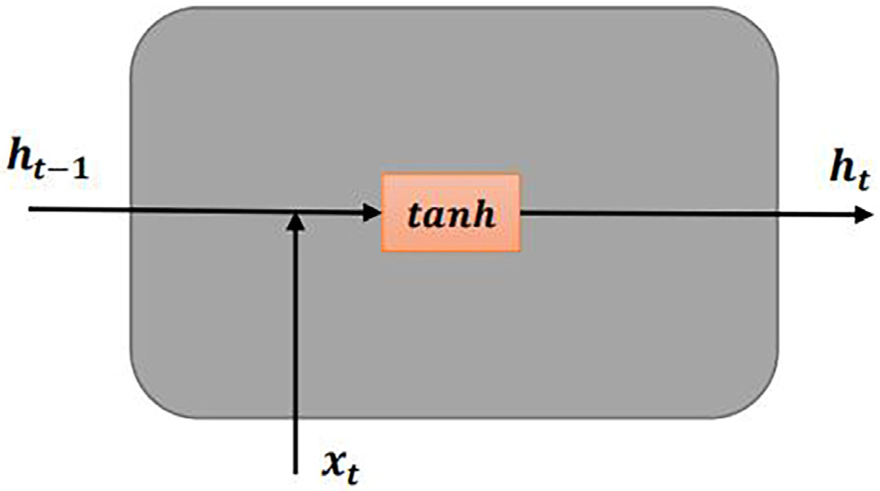
2.1. Recurrent Neural Network (RNN)

Different from BPNN, RNN has a good memory capability of time series and is superior to ordinary neural network in nonlinear relationship fitting of time series data. Therefore, RNN has a good modeling capability in weather prediction, stock prediction, etc. Figure 1 shows the structural unit of the RNN. Traditional neural networks, such as BPNN, can only strictly transfer information from one layer to another in one direction. In RNN, the current state of the model will be affected by its previous state. Its basic unit is a memory cell, and each cell has a number of memory units. The state information h_t at each moment is stored in the memory units and is updated at all times. The update process is shown in the following equation:

$$h_t=tanh\left(x_t·w_{xh}+h_{t-1}·w_{hh}+b_h\right)$$

(1)

where w_xh and w_hh are the weight matrices, b_h is the bias, x_t is the input feature at the current moment, h_t is the status information at the current moment, h_t-1 is the status information at the previous moment, and the function tanh is the hyperbolic function, which is shown in the following equation:

$$f\left(x\right)=\frac{1-e^{-2x}}{1+e^{-2x}}$$

(2)

The output of the current memory cell is as follows:

$$y=h_t·w_{hy}+b_y$$

(3)

where w_hy is the weight matrix, b_y is the bias matrix, which is equivalent to a fully connected layer, and y is the output.

In the RNN, only the number of memory units needs to be set, and it determines the dimension of the weight matrix w_hh. When the number of memory units is specified, and the dimensions of input and output are known, the weight matrices to be trained and the bias dimensions are also determined. During forward propagation, the state information $h_t$ in the memory units is refreshed at every moment. The three weight matrices w_xh, w_hh, and w_hy and the two biases matrix b_h and b_y will not be refreshed. In back propagation, the five matrices to be trained will be updated by gradient descent method.

The disadvantage of RNN is that it cannot solve the long-span dependency problem and can only recall the most recent information, that is, the information perception capability of the previous time node with a large span is insufficient. Therefore, its disadvantage is that it has a short memory time and easily causes gradient explosion and disappearance after multi-stage back propagation. Thus, we attempted to use LSTM to overcome this problem to obtain a more accurate model.

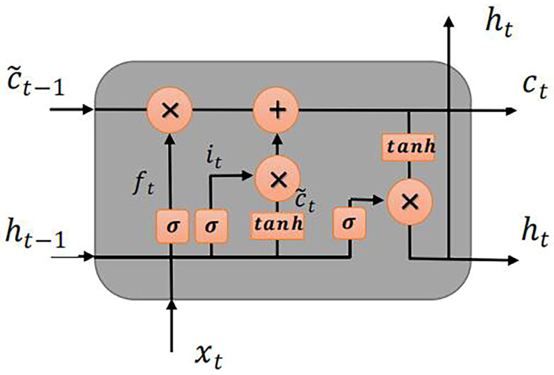
2.2. Long Short-Term Memory (LSTM)

In [31], LSTM, which can learn long-term dependent information, was constructed to solve the gradient explosion and disappearance problems of the traditional RNN. The LSTM unit was composed of input, forget, update, and output gates. The structure of the loop kernel of LSTM can be found in Figure 2, where “×” and “+” represent the multiplication and addition operations of the matrix, respectively, and σ and tanh are the activation functions.

The input gate processes the input of the current sequence position and determines how much information about the input value flows into the current calculation. The input gate i_t is expressed as Equation (4), and the cell information ${\tilde{c}}_t$ is obtained through the tanh activation function, which is expressed as Equation (5). This information may be updated in the cell information in the future.

$$i_t=\sigma \left(w_i·\left[h_{t-1},x_t\right]+b_i\right)$$

(4)

$${\tilde{c}}_t=\tan \mathrm{h}\left(w_c·\left[h_{t-1},x_t\right]+b_c\right)$$

(5)

The forget gate decides whether to forget the state of the upper layer with a certain probability, decides the information to keep, and controls how much information in the historical information flows into the current calculation. The forget gate formula is expressed as the following equation:

$$f_t=\sigma \left(w_f·\left[h_{t-1},x_t\right]+b_f\right)$$

(6)

The principle of the update gate is to forget a part of the old cell information through the forget gate and add cell information ${\tilde{c}}_t$ through the input gate, thereby updating the old cell information ${\tilde{c}}_{t-1}$ to ${\tilde{c}}_t$. The update gate is expressed as the following equation:

$$c_t=f_t·c_{t-1}+i_t·{\tilde{c}}_t$$

(7)

The output gate generates a new long-term memory and calculates the output of the current state. The output gate is expressed as the following equations:

$$o_t=\sigma \left(w_o·\left[h_{t-1},x_t\right]+b_o\right)$$

(8)

$$h_t=o_t·\tanh \left(c_t\right)$$

(9)

Through the interaction of these four steps, the long-term and short-term memories are updated. Thus, the model has the learning capability for time nodes with a large time span. Thus, we can think of the LSTM as an improved algorithm of the RNN. Except for the internal structure of the cell unit, the rest of the operations are the same as those of the RNN. Its appearance was used to improve the model accuracy.

3. Model Establishment

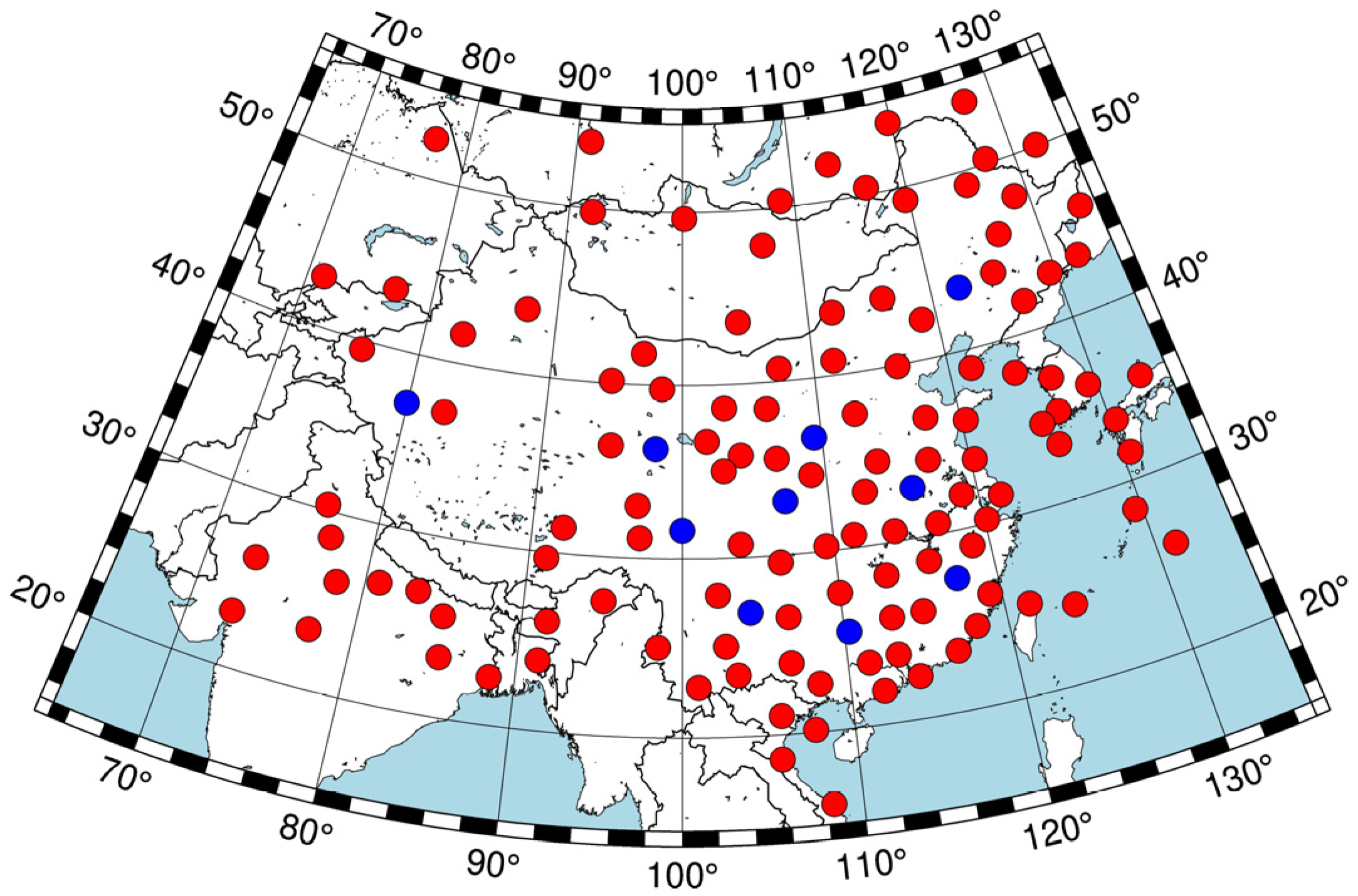
3.1. Data Preparation

To construct the weighted mean temperature model of China, we selected 128 radiosonde stations in China and surrounding areas in the 15° N–55° N and 70° E–135° E regions. Figure 3 shows the specific locations. The red dots are the stations used to train the model and test the prediction performance at modeling stations, and the blue ones are the non-modeling sites, which were used to test the prediction performance at non-modeling stations. Section 5 provides the specific analysis. Meteorological observation data for all stations can be obtained from the Integrated Global Radiosonde Archive (IGRA). We collected 587,893 sets of data for all available weather profiles from 2010 to 2016 to build the model and verified the model accuracy. The Tm value obtained by the radiosonde data integration method was used as the true value and calculated using the following equation:

$$T_m=\frac{{\int }_h^{\infty }\frac{e}{T}dh}{{\int }_h^{\infty }\frac{e}{T^2}dh}$$

(10)

where T is temperature (K), which can be obtained from the sounding data, and e is partial pressure of water vapour (hPa), which is calculated from the relative humidity, and h is the height of the WGS84 ellipsoid, which can be converted from the geopotential height H provided by the sounding data [32,33]. The conversion equations are as follows.

$$\{\begin{array}{c}h=\frac{R\left(\phi \right)·H}{\frac{{\gamma }_s\left(\phi \right)}{{\gamma }_{45}}·R\left(\phi \right)-H}\\ {\gamma }_s\left(\phi \right)={\gamma }_e·\left(\frac{1+ksi{n}^2\phi }{\sqrt{1-e^{2}si{n}^2\phi }}\right)\\ R\left(\phi \right)=\frac{a}{1+f+m-2fsi{n}^2\phi }\end{array}$$

(11)

where h and H are the orthometric height (m) and geopotential height (m) respectively, γ_s(φ) is the acceleration of gravity at latitude φ, and R(φ) is the radius of curvature of the earth at latitude φ. The remaining constants are as follows: a = 6378.137 km; f = 1/298.257223563; m = 0.00344978650684; k = 0.00193185265241; γ_e = 9.7803253359 m/s²; γ₄₅ = 9.80665 m/s²; e² = 6.69437999014 × 10⁻³. The geoid undulation was further calculated by the gravity field model, and the orthometric height was converted into the ellipsoidal height.

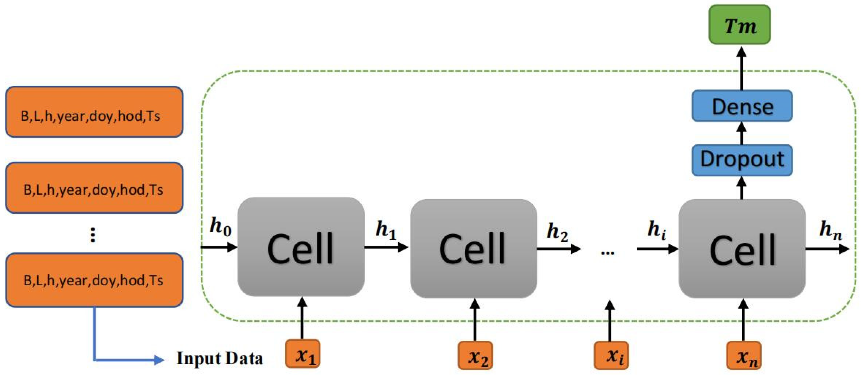
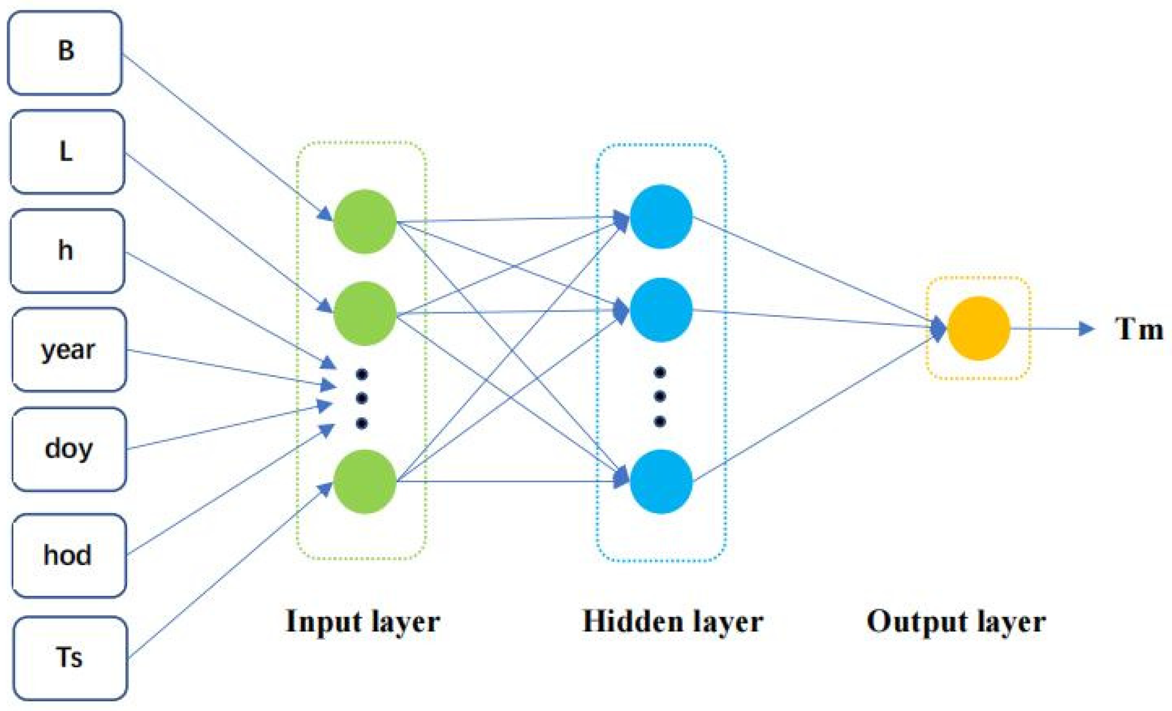
3.2. Input and Output of the Model

Tm has a strong correlation with temperature and water vapor pressure, but the water vapor pressure is often inconvenient to obtain in actual measurement. Therefore, we considered only the meteorological element temperature (Ts) as a part of the input value of the model to enable users to use the model in actual measurements. In addition, for the model to have a high spatial and temporal resolution, we added time information (year, day of year (doy), and hour of day (hod)) and spatial information (latitude, longitude, and altitude). The output of the model selects the high-precision Tm value obtained by the numerical integration of radiosonde data. Through deep learning algorithms, the complex linear relationship between the input and output was simulated and constructed. The relationship between the input variables and output Tm of the model can be written as:

$$Tm=f\left(lat, lon, h, year, doy, hod, Ts\right)$$

(12)

Figure 4 shows the model structure, and the model input was the x_i value passed into the cell module, where x_i = (latitude, longitude, altitude, year, doy, hod, Ts). The cell module is the memory cell units of RNN and LSTM mentioned in Section 2. Variable h_i stores the memory information of each moment and connects each cell unit. Finally, the predicted value was the output obtained through a dropout layer and a dense layer. The dropout layer sparses w_hy in Equation (3), thereby alleviating overfitting. In this model, the time step was 4, that is, n = 4. Dropout = 0.2, which means that 20% of the matrix elements were randomly returned to 0. The dense layer is equivalent to a fully connected layer of the BPNN. Given that the model output has one Tm value, it was set to 1 to output the final predicted value.

3.3. Data Normalization

Multi-parameter input models usually have different dimensions and orders of magnitude given the varied nature of various inputs. When the magnitude of each input differs greatly, direct modeling with the original data will highlight the role of indicators with high values in modeling. Therefore, the original data must be standardized to ensure the accuracy of results. The following equation shows the maximum and minimum normalization strategy used in this article:

$$X_N=\frac{2\left(X-X_{min}\right)}{X_{max}-X_{min}}-1$$

(13)

where X_N is the value after normalization, X is the original value, and X_min and X_max are the minimum and maximum values, respectively. After the above formula calculation, the original value can be normalized to values between −1 and +1.

3.4. Determination of Model Hyperparameters

The scripts were written based on tensorflow2.1 package of Python (3.7), and the Adam gradient descent algorithm was used to update the parameters. Adam optimization is a stochastic gradient descent method based on the adaptive estimation of first-order and second-order moments [34]. Given its excellent performance, this method has been widely used, and it can adaptively adjust the learning rate to reach the local optimal value of the loss function and iterate based on the training data to update the weights of neural networks.

First, we need to determine the number of memory units of two models. This step is equivalent to determining the number of neurons in the hidden layer. The number of experimental memory units ranged from 5 to 100, and the step length was 5. We recorded the RMSE value of each experiment and plotted the relationship between the number of experimental memory units and RMSE in Figure 5. The best performance was obtained when the number of memory units of the RNN_Tm and LSTM_Tm models were 30 and 75, respectively.

After we got the best memory numbers for the two models, in order for the models to have better performance, we need to further adjust the hyperparameters. There are many methods for gradient descent. We finally chose the Adam algorithm as the optimizer of the model, because the Adam algorithm can make it more convenient for us to adjust the hyperparameters, and only need to set the initial learning rate instead of setting the learning rate decay rate. It can adaptively adjust the learning rate to find the local minimum of the loss function. Experiments have also proved that using Adam can quickly find the optimal value after fewer epochs. We set the initial learning rate ranged from 0.001 to 0.01, and the step length is 0.001, hoping to find the best initial learning rate through detailed experiments. At the same time, in order to alleviate overfitting, we use the “Dropout” method, which can sparse the weight matrix by a certain ratio. We set dropout ranged from 0.1 to 0.5, with a step length of 0.1, and find the best dropout value through experiments. Both models are set to epochs = 100, and the optimal number of epochs is determined by accessing the optimal model. We recorded the final hyperparameters in

Table 1. Optimal hyperparameters of the two models.

Model	Memory Unit Number	Learning Rate	Dropout	Epochs
RNN_Tm	30	0.001	0.2	43
LSTM_Tm	75	0.005	0.2	27

. The best RMSE values of the RNN_Tm model and LSTM_Tm model are 3.01 K and 2.89 K, respectively.

4. Model Evaluation

4.1. Model for Comparison

4.1.1. BTm Model

To verify its accuracy, we compared the constructed model with the BTm and GPT3 models. The BTm model showed the linear relationship between Tm and the temperature (T_s) of the station, as observed by Bevis et al. [3] through 8718 radiosonde profiles at 13 sounding stations distributed in the United States. The expression is shown in the following equation:

$$Tm=70.2+0.72·T_s$$

(14)

4.1.2. GPT3 Model

The GPT3 model is an empirical model that provides grid data of 5° × 5° and 1° × 1°. In addition to providing meteorological data, such as temperature, pressure, and water vapor pressure, it can also be used to calculate the Tm value. The data used in this paper were 1° × 1° grid data. The GPT3 model considers the characteristics of annual and semi-annual cycles, and its formula is shown in the following equation:

$$\begin{array}{c}X=A_0+A_1·\cos \left(\frac{doy}{365.25}2\pi \right)+B_1\sin \left(\frac{doy}{365.25}2\pi \right)+\\ A_2·\cos \left(\frac{doy}{365.25}4\pi \right)+B_2\sin \left(\frac{doy}{365.25}4\pi \right)\end{array}$$

(15)

where X is the meteorological parameter, doy is the day of year, $A_0$ is the average value, $A_1$ and $B_1$ are the annual amplitudes, and $A_2$ and $B_2$ are the half-year amplitudes.

4.1.3. BPNN Model

The BPNN model is one of the most commonly used machine learning algorithms. At present, more weighted average temperature and machine learning combined modeling often use this method. It consists of three parts: input layer, hidden layer, and output layer. BPNN uses a gradient descent method to update the connection weights between layers to find the local optimal value of the loss function.

The structure of BPNN is shown in Figure 6. We use the same modeling strategy as in Section 3 to build the BPNN model, using the Adam optimizer as the gradient descent method. After experimentation, we choose the initial learning rate to be 0.001, the number of hidden layers to be 15, and the best epoch number to be 90.

4.2. Model Evaluation Index

In this article, the performance of the model is evaluated by calculating the root mean square error (RMSE), mean absolute error (MAE), bias, and correlation coefficient (R). The formulas are shown in the following equations:

$$RMSE=\sqrt{\frac{1}{N}{\displaystyle \sum }_{i=1}^N{\left(T_{m_i}^{model}-T_{m_i}^{real}\right)}^2}$$

(16)

$$MAE=\frac{1}{N}{\displaystyle \sum }_{i=1}^N\left|T_{m_i}^{model}-T_{m_i}^{real}\right|$$

(17)

$$Bias=\frac{1}{N}{\displaystyle \sum }_{i=1}^N\left(T_{m_i}^{model}-T_{m_i}^{real}\right)$$

(18)

$$R=\frac{{\displaystyle \sum _{i=1}^N(T_{m,i}^{model}-\overline{T_{m,i}^{model}})(T_{m,i}^{real}-\overline{T_{m,i}^{real}})}}{\sqrt{{\displaystyle \sum _{i=1}^N{}_i{(T_{m,i}^{model}-\overline{T_{m,i}^{model}})}^2{\displaystyle \sum _{i=1}^N{}_i{(T_{m,i}^{real}-\overline{T_{m,i}^{real}})}^2}}}}$$

(19)

$$KGE=1-\sqrt{{\left(R-1\right)}^2+{\left(\frac{{\sigma }_{model}}{{\sigma }_{real}}-1\right)}^2+{\left(\frac{{\mu }_{model}}{{\mu }_{real}}-1\right)}^2}$$

(20)

where N is the total number of samples, $T_{m_i}^{model}$ is the Tm value calculated by the model, and $T_{m_i}^{real}$ is the high-precision Tm value calculated by the radiosonde data using numerical integration, σ_real is the standard deviation in observations, σ_model is the standard deviation in simulations, µ_model is the simulation mean, µ_real is the observation mean.

4.3. Computational Performance of the Model

In addition to verifying the accuracy of machine learning performance, another important factor is the evaluation of the model’s computational performance, that is, the model complexity. The experiment was implemented on a Spyder interpreter. In the experiment, we attempted to use Nvidia’s CUDA for GPU acceleration, but the effect was not evident. Thus, the CPU was used to run the entire program. The computer CPU was configured with Core i7-7700HQ at 2.8 GHz. We recorded the time consumption and predicted time consumption of the entire training phase of the model and recorded the number of model parameters.

Table 2. Training and prediction times and the number of parameters of the different models.

Model	Training Time	Prediction Time	Parameter Numbers
RNN_Tm	11′54″	0′02″	1171
LSTM_Tm	15′35”	0′04″	24,976
BPNN	25″49	0′02″	135
GPT3	-	0′03″	324,000

records the computational performance of the RNN_Tm, LSTM_Tm, BPNN, and GPT3models.

Table 2 shows the long training time of the two deep learning algorithms (10–20 min) resulting from the extremely large total number of input samples, including 537,893 sets of data, in the model training stage. The training process involved considerable calculation and parameter updating processes. However, the prediction times of the two models were notably short. RNN_Tm and LSTM_Tm required 2 and 4 s to predict the results, respectively, because only simple forward calculations were needed to predict the results after the optimal parameters were obtained by model training. At the same time, we found that the parameters of the BPNN model are the least because of its simpler model structure. Since GPT3 is a grid model, the number of its parameters is very huge. Comparing the two models, the LSTM_Tm model required more training and prediction time, and the number of parameters was greater than that of RNN_Tm due to the difference in the structure of the memory cell of the two neural networks. The RNN has a simple structure, whereas the memory cell of LSTM is more complex, including update, input, forget, and output gates. The model precision of the LSTM was improved through these gate control units.

5. Results

5.1. Predictive Performance of the Model at Modeling Stations

In this paper, the deep learning methods RNN and LSTM were used to build two models using the data set of 118 sounding stations provided by the IGRA. The data from 2010 to 2015 were used to train the model, and the data from 2016 were used to test the prediction performance of the models at modeling stations.

Table 3. Performance evaluation index of different models.

Model	RMSE	Bias	MAE	R	KGE
BTm	4.34	0.57	3.35	0.935	0.806
GPT3	4.37	−0.88	3.38	0.932	0.892
BPNN	3.48	0.34	2.57	0.921	0.924
RNN_Tm	3.01	−0.13	2.33	0.967	0.942
LSTM_Tm	2.89	0.14	2.23	0.970	0.954

shows the performance comparison between the obtained three models and the BTm model, the GPT3 model and BPNN model. Table 3 also reveals that the bias of the two newly constructed models is close to 0, which is a good calibration of the system deviation of the traditional model. Compared with the GPT3 model, the RMSE values of the RNN_Tm and LSTM_Tm models were reduced by 31.1% and 33.9%, respectively. Both deep learning methods greatly reduced the RMSE of the model. The correlation coefficient of the newly constructed model was also higher than that of the traditional method, reaching about 0.97, which also reflects that compared with traditional modeling ideas, the deep learning modeling method can better fit the complex nonlinear relationship within the model. The KGE value integrates the correlation coefficient R, bias, and a measure of relative variability to evaluate the overall performance of the model. The results also show that the two newly constructed models have better accuracy than the BPNN model. The KGE values of the two newly constructed models were 0.942 and 0.954, respectively. Compared with the two traditional models, the overall performance of the model has been greatly improved. The accuracy of the LSTM_Tm model was significantly better than that of the RNN_Tm model because the LSTM method solves the shortcomings of the RNN method, including the insufficient information perception capability for the previous time nodes with a large span, and has a naturally better model performance than the RNN model.

We used the constructed RNN_Tm model, LSTM_Tm model, and two empirical models for comparison to calculate the 2016 Tm data and the respective RMSE of 118 sounding stations. Figure 7 shows the plotted RMSE values of each station. In the comparison of the four models, the LSTM_Tm and RNN_Tm models showed better performance than the GPT3 and BTm models, with the LSTM_Tm model exhibiting the best effect. In addition, the RMSE value distributions of the four models all showed that the RMSE of low-latitude areas was generally better than that of high-latitude areas because the Tm of high-latitude areas has stronger seasonal changes. Thus, the modeling accuracy was lower than that of low-latitude areas. We observed that the accuracy of the GPT3 and BTm models was high at low latitudes, which is equivalent to the accuracy of the RNN_Tm and LSTM_Tm models. However, the two empirical models showed poor accuracy in areas with latitudes greater than 30°. By analyzing Figure 7a,b, we discovered that although the two deep learning models (RNN_Tm and LSTM_Tm) presented a poor high-latitude accuracy, compared with the GPT3 and BTm models, the RMSE value distribution of the two newly constructed models was more uniform, indicating that the generalization of deep learning models is better than that of the traditional empirical models.

We also analyzed the performance of the models between different latitude zones and calculated the RMSE values of the four models every 5° (

Table 4. RMSE of Various Models in Different Latitude Zones [K].

Latitude	BTm	GPT3	RNN_Tm	LSTM_Tm
15° N–20° N	3.74	2.75	2.33	2.13
20° N–25° N	3.47	2.96	2.23	2.21
25° N–30° N	3.71	3.56	2.60	2.53
30° N–35° N	3.97	4.37	2.91	2.79
35° N–40° N	4.45	4.67	3.28	3.11
40° N–45° N	4.80	5.09	3.45	3.25
45° N–50° N	4.61	4.85	3.31	3.20
50° N–55° N	5.61	5.20	3.71	3.59

and Figure 8). As the latitude increased, the RMSE values of all the models also increased due to the strong seasonal changes in high-latitude areas and large changes in water vapor. However, the RNN_Tm and LSTM_Tm models were less affected by the latitude factor. In all latitude zones, the RMSE was smaller than that of the GPT3 and BTm models. Training proved that through with a large amount of data, the two models can alleviate the poor modeling accuracy of weighted mean temperature in high-latitude areas due to seasonal factors. In addition, the accuracy of the LSTM_Tm model was slightly better than that of the RNN_Tm model because LSTM is an improved algorithm of the RNN model, and the LSTM_Tm model has a better predictive capability.

By analyzing Figure 8, we determined that compared with the GPT3 and BTm models, the RMSE values of the two deep learning models varied more uniformly with latitude. Table 4 shows that the RMSE values of the GPT3 and BTm models ranged from 2.75 K to 5.20 K and from 3.75 K to 5.61 K, respectively. The RMSE ranges of the deep learning RNN_Tm and LSTM_Tm models were 2.32 K to 3.75 K and 2.11 K to 3.50 K, respectively. Thus, the deep learning algorithm and the method of using the station coordinate information as the input to train the model can ensure the uniform high-precision prediction ability of the model in each latitude interval.

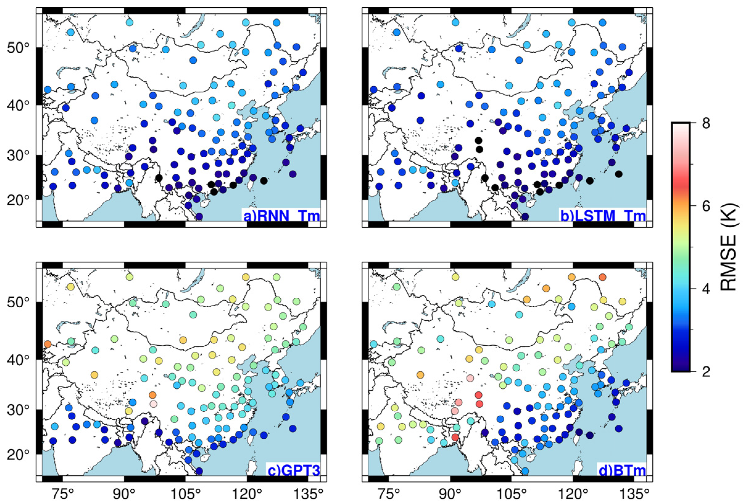
5.2. Predictive Performance of Model at Non-Modeling Stations

In Section 5.1, we analyzed the prediction performance of the 2016 data of 118 stations where the model was established and concluded that the model has a good performance at modeling stations. Then, we considered whether other sites in the Chinese region have good generalization in addition to these sites for model construction. In this part, we selected 10 evenly distributed sites in China, which are different from the 118 modeling sites, and used the built deep learning models (RNN_Tm and LSTM_Tm) to predict their Tm values from 2010 to 2016. Two traditional models were used to calculate Tm values for comparison, and their respective RMSE values were counted (

Table 5. RMSE of four models at different stations [K].

Station	Latitude(°)	Longitude(°)	H(m)	BTm	GPT3	RNN_Tm	LSTM_Tm
57957	25.33	110.30	166	2.79	3.50	2.30	2.45
56691	26.87	104.28	2236	2.51	4.02	2.58	2.97
58725	27.33	117.47	219	3.06	3.49	2.47	2.28
56146	31.62	100.00	3394	6.02	4.05	2.29	2.29
58203	32.87	115.73	33	3.59	4.36	3.25	3.25
57127	33.07	107.03	509	3.10	5.47	2.93	2.72
52836	36.30	98.10	3190	7.75	3.79	2.67	2.64
53845	36.57	109.45	959	4.52	4.39	3.67	3.23
51828	37.14	79.93	1375	6.17	4.27	3.10	2.86
54135	43.60	122.27	180	5.34	5.36	3.80	3.71
Mean	-	-	-	4.49	4.27	2.91	2.84

and Figure 9).

Table 5 shows that the performance of the two deep learning models at non-modeling points was better than that of the traditional models overall. For the 10 test sites, the average RMSE of the traditional BTm and GPT3 models were 4.49 K and 4.27 K, respectively. The average RMSEs of the RNN and LSTM based on deep learning were 2.91 K and 2.84 K, respectively. Figure 9 shows that the accuracy of the BTm and GPT3 models was uneven at different stations. The accuracy of the BTm model in seven stations was higher than that of the GPT3 model, whereas that of the other three stations was significantly lower than that of the GPT3 model. Thus, the generalization of the two comparative models was low, and the TM prediction capability in different locations varied greatly. By contrast, the RMSE values of the RNN_Tm and LSTM_Tm models varied more evenly at these 10 stations. In general, the new models retain a good prediction performance at non-modeling stations.

To further analyze the model performance, we plotted the RMSE values of the four models of these 10 sites (Figure 10). The findings were the same as the results presented in Section 5.1. The RNN_Tm and LSTM_Tm models overcome the shortcomings of poor generalization of traditional empirical model due to high latitude and seasonal changes and maintain a good TM prediction performance in the whole region of China.

As shown Figure 11, we selected station 57127, compared the Tm value calculated by the BTm, GPT3, RNN, and LSTM models with the high-precision Tm value obtained based on the numerical integration of radiosonde data, and plotted the Tm time series diagram from 2010 to 2016. The BTm model was fitted based on the relationship between the Tm value and temperature, and it showed a certain degree of reliability. However, in general, the prediction performance of the BTm model in winter in China was poorer than that in summer because it only fits the linear relationship between the Tm value and temperature and disregards the influence of geographical location on Tm. Although the empirical GPT3 model considers the location factors of the station and simulates the seasonal Tm changes well, the Tm changes have a strong correlation with meteorological factors. Reflecting deep Tm and complex meteorological factors through the GPT3 model was difficult, which led to its low accuracy in China. The two newly constructed deep learning models (RNN_Tm and LSTM_Tm), by constructing the relationship between Tm, space-time information, and temperature T, can fit the complex nonlinear relationship well, which is one of the reasons for their high accuracy.

We selected four stations and analyzed the residual time series diagrams of the four models from 2010 to 2016 (Figure 12). The residuals of the BTm and GPT3m models showed a seasonal change. In general, the deviation value in winter was larger, which is also consistent with the above analysis. In addition, the predicted value of the BTm model generally showed a large positive residual (Figure 12a,b). The reason was analyzed because the elevation values of these two stations were relatively large, at 3190 and 3394 m respectively. The BTm model showed a large positive residual in high-altitude areas because it disregards the station location. Furthermore, the BTm model only considers the relationship between the Tm and temperature, while high-altitude areas have less water vapor, leading to a large Tm estimate. For the GPT3 model, the four stations showed a certain degree of negative residual, which indicates that the global-experience GPT3 model has a systematic deviation in China.

In addition, we counted the distribution of all the residual values of four stations from 2010 to 2016 and observed that the proportions of the residual values of the BTm, GPT3, RNN_Tm, and LSTM_Tm models between (−5 K, 5 K) were 56%, 75%, 93%, and 95%, respectively. Most of the residual values of the RNN and LSTM models were within (−5 K, 5 K), which indicates the notably high prediction accuracy of the RNN_Tm and LSTM_Tm models. Figure 12 shows that the residual changes in the RNN_Tm and LSTM_Tm models were relatively stable. Thus, both models were not affected by location altitude and seasonal changes because we added the time and coordinate information as the input values of the model in model training. Through multiple training epochs, the RNN_Tm and LSTM_Tm models fitted well the complex nonlinear relationship between the input and Tm values. Therefore, the overall residual of two deep learning models was small, which is difficult to achieve by the traditional empirical model.

6. Conclusions

In this research, we applied deep learning modeling to Tm modeling and proposed a novel modeling strategy based on RNN and LSTM to build high-precision Tm models. We used data from 118 radiosonde stations in and around China from 2010 to 2015 to train the model and used the 2016 data from these stations to test the model’s Tm prediction performance at modeling stations. The RMSE values of the RNN and LSTM models were 3.01 K and 2.89 K, respectively. Compared with the widely used global-experience GPT3 model, the prediction accuracy was improved by 31.1% and 33.9%. By comparing the accuracy of the models in different latitude zones, we observed that deep learning models are better than traditional empirical models in overcoming the large Tm estimation error caused by high-latitude factors. In addition, to verify the prediction performance of the two models at non-modeled points in China, we selected the data of another 10 radiosonde stations from 2010 to 2016 to test their accuracy, and the RMSE values obtained were 2.95 K and 2.86 K, respectively. The applicability and accuracy of the model in all positions in the modeling area were guaranteed. We analyzed the residual time series diagrams of two traditional empirical models (BTm and GPT3 models) and two deep learning models (RNN_Tm and LSTM_Tm models), and compared with the traditional model, the deep learning models alleviated the effect of altitude and seasonal changes on the model accuracy. Since the two newly constructed models also have good generalization in non-modeling sites, the models have good transferability.

The application of deep learning to Tm modeling is highly advantageous. The reason can be explained by the use of multi-parameter input to build the model. Longitude, latitude, elevation, time parameters, temperature were all used to simulate the relationship with the output Tm value. Through the training of a large amount of data, the model fitted the complex nonlinear relationship between the input and output. Thus, the model has a good Tm prediction capability. Another advantage of the model is that it only needs to measure the temperature of the site as a meteorological element to obtain a high-precision Tm prediction value, which is convenient for users. China was considered the research area in this article. In future work, we will use deep learning algorithms to model global data and will not be limited to the Tm prediction on the surface of the research site.

References

1. Davis, J.L.; Herring, T.A.; Shapiro, I.I.; Rogers, A.E.E.; Elgered, G. Geodesy by radio interferometry: Effects of atmospheric modeling errors on estimates of baseline length. Radio Sci. 1985, 20, 1593–1607. [Google Scholar] [CrossRef]
2. Bevis, M.; Businger, S.; Herring, T.A.; Rocken, C.; Anthes, R.A.; Ware, R.H. GPS meteorology: Remote sensing of atmospheric water vapor using the global positioning system. J. Geophys. Res. Atmos. 1992, 97, 15787–15801. [Google Scholar] [CrossRef]
3. Bevis, M.; Businger, S.; Chiswell, S.; Herring, T.A.; Ware, R.H. GPS Meteorology: Mapping Zenith Wet Delays onto Precipitable Water. J. Appl. Meteorol. 1994, 33, 379–386. [Google Scholar] [CrossRef]
4. Yao, Y.; Zhang, B.; Xu, C.; Chen, J. Analysis of the global Tm–Ts correlation and establishment of the latitude-related linear model. Chin. Sci. Bull. 2014, 59, 2340–2347. [Google Scholar] [CrossRef]
5. Baldysz, Z.; Nykiel, G. Improved Empirical Coefficients for Estimating Water Vapor Weighted Mean Temperature over Europe for GNSS Applications. Remote Sens. 2019, 11, 1995. [Google Scholar] [CrossRef] [Green Version]
6. Yao, Y.; Zhu, S.; Yue, S. A globally applicable, season-specific model for estimating the weighted mean temperature of the atmosphere. J. Geod. 2012, 86, 1125–1135. [Google Scholar] [CrossRef]
7. Yao, Y.; Zhang, B.; Yue, S.; Chao, Q.; Wen, F. Global empirical model for mapping zenith wet delays onto precipitable water. J. Geod. 2013, 87, 439–448. [Google Scholar] [CrossRef]
8. Yao, Y.; Xu, C.; Zhang, B.; Cao, N. GTm-III: A new global empirical model for mapping zenith wet delays onto precipitable water vapour. Geophys. J. Int. 2018, 197, 202–212. [Google Scholar] [CrossRef] [Green Version]
9. Bhm, J.; Mller, G.; Schindelegger, M.; Pain, G.; Weber, R. Development of an improved empirical model for slant delays in the troposphere (GPT2w). GPS Solut. 2015, 19, 433–441. [Google Scholar] [CrossRef] [Green Version]
10. Landskron, D.; Boehm, J. VMF3/GPT3: Refined discrete and empirical troposphere mapping functions. J. Geod. 2018, 92, 349–360. [Google Scholar] [CrossRef]
11. Sun, Z.; Zhang, B.; Yao, Y. A Global Model for Estimating Tropospheric Delay and Weighted Mean Temperature Developed with Atmospheric Reanalysis Data from 1979 to 2017. Remote Sens. 2019, 11, 1893. [Google Scholar] [CrossRef] [Green Version]
12. Chen, P.; Yao, W.; Zhu, X. Realization of global empirical model for mapping zenith wet delays onto precipitable water using NCEP re-analysis data. Geophys. J. Int. 2014, 198, 1748–1757. [Google Scholar] [CrossRef] [Green Version]
13. Zhang, H.; Yuan, Y.; Li, W.; Ou, J.; Li, Y.; Zhang, B. GPS PPP-derived precipitable water vapor retrieval based on Tm/Ps from multiple sources of meteorological data sets in China. J. Geophys. Res. 2017, 122, 4165–4183. [Google Scholar] [CrossRef]
14. Balidakis, K.; Nilsson, T.; Zus, F.; Glaser, S.; Heinkelmann, R.; Deng, Z.; Schuh, H. Estimating Integrated Water Vapor Trends From VLBI, GPS, and Numerical Weather Models: Sensitivity to Tropospheric Parameterization. J. Geophys. Res. Atmos. 2018, 123, 6356–6372. [Google Scholar] [CrossRef] [Green Version]
15. Li, Q.; Chen, P.; Sun, L.; Ma, X. A global weighted mean temperature model based on empirical orthogonal function analysis. Adv. Space Res. 2018, 61, 1398–1411. [Google Scholar] [CrossRef]
16. Huang, L.; Jiang, W.; Liu, L.; Chen, H.; Ye, S. A new global grid model for the determination of atmospheric weighted mean temperature in GPS precipitable water vapor. J. Geod. 2019, 93, 159–176. [Google Scholar] [CrossRef]
17. Huang, L.; Liu, L.; Chen, H.; Jiang, W. An improved atmospheric weighted mean temperature model and its impact on GNSS precipitable water vapor estimates for China. GPS Solut. 2019, 23, 51. [Google Scholar] [CrossRef]
18. Li, Q.; Yuan, L.; Chen, P.; Jiang, Z. Global grid-based Tm model with vertical adjustment for GNSS precipitable water retrieval. GPS Solut. 2020, 24, 73. [Google Scholar] [CrossRef]
19. Ding, M. A neural network model for predicting weighted mean temperature. J. Geod. 2018, 92, 1187–1198. [Google Scholar] [CrossRef]
20. Ding, M. A second generation of the neural network model for predicting weighted mean temperature. GPS Solut. 2020, 24, 61. [Google Scholar] [CrossRef]
21. Yang, L.; Chang, G.; Qian, N.; Gao, J. Improved atmospheric weighted mean temperature modeling using sparse kernel learning. GPS Solut. 2021, 25, 28. [Google Scholar] [CrossRef]
22. Sun, Z.; Zhang, B.; Yao, Y. Improving the Estimation of Weighted Mean Temperature in China Using Machine Learning Methods. Remote Sens. 2021, 13, 1016. [Google Scholar] [CrossRef]
23. Gill, M.K.; Asefa, T.; Kemblowski, M.W.; Mckee, M. Soil moisture prediction using support vector machines. JAWRA J. Am. Water Resour. Assoc. 2006, 42, 1033–1046. [Google Scholar] [CrossRef]
24. Lv, H.; Chen, G. Research on Wind Speed Vertical Extrapolation Based on Extreme Learning Machine; Springer: Singapore, 2017; pp. 3–11. [Google Scholar] [CrossRef]
25. Bhuiyan, A.E.; Yang, F.; Biswas, N.K.; Rahat, S.H.; Neelam, T.J. Machine Learning-Based Error Modeling to Improve GPM IMERG Precipitation Product over the Brahmaputra River Basin. Forecasting 2020, 2, 248–266. [Google Scholar] [CrossRef]
26. Yaseen, Z.M.; Sulaiman, S.O.; Deo, R.C.; Chau, K.W. An enhanced extreme learning machine model for river flow forecasting: State-of-the-art, practical applications in water resource engineering area and future research direction. J. Hydrol. 2019, 569, 387–408. [Google Scholar] [CrossRef]
27. Ahn, K.H.; Palmer, R. Regional flood frequency analysis using spatial proximity and basin characteristics: Quantile regression vs. parameter regression technique. J. Hydrol. 2016, 540, 515–526. [Google Scholar] [CrossRef]
28. Tyralis, H.; Papacharalampous, G.; Burnetas, A.; Langousis, A. Hydrological post-processing using stacked generalization of quantile regression algorithms: Large-scale application over CONUS. J. Hydrol. 2019, 577, 123957. [Google Scholar] [CrossRef]
29. Asanjan, A.A.; Yang, T.T.; Hsu, K.L.; Sorooshian, S.; Lin, J.Q.; Peng, Q.D. Short-Term Precipitation Forecast Based on the PERSIANN System and LSTM Recurrent Neural NetworksN. J. Geophys. Res. Atmos. 2018, 123, 12543–12563. [Google Scholar] [CrossRef]
30. Zhang, Q.; Wang, H.; Dong, J.Y.; Zhong, G.Q.; Sun, X. Prediction of Sea Surface Temperature Using Long Short-Term Memory. IEEE Geosci. Remote Sens. Lett. 2017, 14, 1745–1749. [Google Scholar] [CrossRef] [Green Version]
31. Hochreiter, S.; Schmidhuber, J. Long Short-Term Memory. Neural Comput. 1997, 9, 1735–1780. [Google Scholar] [CrossRef]
32. Dousa, J.; Elias, M. An improved model for calculating tropospheric wet delay. Geophys. Res. Lett. 2014, 41, 4389–4397. [Google Scholar] [CrossRef]
33. Wang, X.; Zhang, K.; Wu, S.; Fan, S.; Cheng, Y. Water vapor-weighted mean temperature and its impact on the determination of precipitable water vapor and its linear trend. J. Geophys. Res. Atmos. 2016, 121, 833–852. [Google Scholar] [CrossRef]
34. Kingma, D.; Ba, J. Adam: A Method for Stochastic Optimization. arXiv 2014, arXiv:1412.6980. [Google Scholar]
Figure 1. The structure of Simple Recurrent Neural Network (RNN) cell.
Remotesensing 13 03004 g001
Figure 2. The structure of Long-Short Term Memory (LSTM) cell.
Remotesensing 13 03004 g002
Figure 3. Distribution of radiosonde stations in China. The dots denote the positions of the stations.
Remotesensing 13 03004 g003
Figure 4. The structure of RNN and LSTM models.
Remotesensing 13 03004 g004
Figure 5. Relationship between the RMSE of the two models and the number of memory units in the model. (a) LSTM model, (b) RNN model.
Remotesensing 13 03004 g005
Figure 6. The structure of BPNN model.
Remotesensing 13 03004 g006
Figure 7. RMSE distribution of the four models at each radiosonde station. (a) RNN_Tm, (b) LSTM_Tm, (c) GPT3, and (d) BTm models.
Remotesensing 13 03004 g007
Figure 8. RMSE of various models in different latitude zones.
Remotesensing 13 03004 g008
Figure 9. RMSEs of different models at 10 stations (K).
Remotesensing 13 03004 g009
Figure 10. Distribution of the RMSEs of the four models at 10 non-modeling stations. (a) RNN_Tm, (b) LSTM_Tm, (c) GPT3, and (d) BTm models.
Remotesensing 13 03004 g010
Figure 11. Tm time series calculated from four models and radiosonde observations at station 57127.
Remotesensing 13 03004 g011
Figure 12. Residuals of the LSTM_Tm (red), RNN_Tm (yellow), BTm (green), and GPT3 (blue) models of four radiosonde stations in China from 2010 to 2016. (a) 52386, (b) 56146, (c) 57127, and (d) 51828 stations.
Remotesensing 13 03004 g012