RSPD: A Novel Remote Sensing Index of Plant Biodiversity Combining Spectral Variation Hypothesis and Productivity Hypothesis

Abstract

Plant diversity (PD) plays an important role in maintaining the healthy function of an ecosystem through affecting the productivity, stability, and nutrient utilization of a terrestrial ecosystem. Remote sensing is a vital way to monitor the status and changes of PD. Most of the existing methods rely on a field botany survey to construct a statistical relationship between PD and remote sensing observations. However, a field botany survey is too costly to be applied widely. In this study, we constructed a new remote sensing index of PD (RSPD), combining the spectral variation hypothesis and productivity hypothesis. Concretely, the RSPD integrated the multi-band spectral reflectance and several spectral greenness, moisture, and red-edge vegetation indices with the principles of Shannon information entropy and Euclidean distance. The RSPD was evaluated by comparing the classical coefficient of variation (CV) method and the Shannon and Simpson diversity indices based on vegetation classification results. Two cases were selected, where Case I was in Beijing and Case II was located in part of Huai’an, China. Sentinel-2 data in three years of 2016, 2018, and 2020 and higher-resolution Pléiades-1 data in 2018 were also utilized. The results demonstrate that: (1) the RSPD is basically consistent with the CV in spatiotemporal variation; (2) the RSPD outperforms the CV as compared with Shannon and Simpson diversity indices that are based on vegetation classification results with Sentinel-2 and Pléiades-1 data; (3) the RSPD outperforms the CV as compared with visual interpretations with Google Earth image. The suggested index can reflect the richness and evenness of plant species, which is inherent in its calculation formula. Moreover, it has a great potential for large-scale regional and long-term series monitoring.

1. Introduction

Plant biodiversity chiefly refers to the species richness and abundance of plants in a measurement area. Plant biodiversity plays a critical role in maintaining healthy ecosystem function because of its influences on ecosystem productivity, community and ecosystem stability, invasibility, and nutrient use and retention [1,2]. Currently, biodiversity has become an important social and scientific issue with widespread international concern. For example, about 196 nations have ratified the Convention on Biological Diversity, an international legal instrument for the conservation of biological diversity. However, with rapid urbanization and population growth, some human activities destroyed the natural environment, caused the loss of species and habitats, and brought serious threats to the protection of biodiversity [3]. Therefore, biodiversity has become an issue of widespread international concern. In order to effectively protect biodiversity, it is necessary to monitor its status and changes in a timely, spatial continuous, and dynamic manner.

Field surveying of plant biodiversity is almost infeasible for every study area at the landscape scale, regional scale or even the global scale [4,5]. Since the 1990s, remote sensing technology has been widely utilized for plant biodiversity, because of the inherent technical characteristics of wide coverage, and consistent and repeatable measurement in an efficient and cost-effective way [2,6,7,8]. Wang and Gamon [2] reviewed the remote sensing of terrestrial plant biodiversity and classified the studies into four categories: (1) mapping distributions of species or functional types, (2) estimating biodiversity through plant functional traits, (3) estimating biodiversity through habitat mapping, and (4) estimating biodiversity through spectral diversity. The first way is a direct method that requires fine spectral and spatial resolutions for direct species mapping. However, most satellite data are too coarse to map the distributions of species directly. Plant functional traits can be defined as quantifiable morpho-physio-chemical-phenological traits of individual organisms that present a response to the variation of environment and its effects on growth, reproduction, organism survival, and ecosystem processes [9]. Typical functional traits include leaf area, leaf nitrogen concentration, leaf dry matter content, plant maximum height, canopy shape index, and phenology (peak fruiting), etc. [10]. Although remote sensing has been applied to detect plant functional traits, there are still many challenges in detection, such as the adverse effect of soil reflectance, seasonal change, and high variability of plant traits [2]. Habitat mapping methods are generally based on a hypothesis that habitat heterogeneity positively correlates with biodiversity [11,12,13]. In this way, remote sensing often provides environmental indicators related to climate and habitat structure, geology and topography, such as temperature [14], fractional vegetation coverage, or spectral vegetation indices [15,16,17,18], net primary productivity [19], and land cover types [20]. However, habitat mapping is highly scale-dependent and is affected by the characteristics of the species involved. Moreover, this approach usually ignores within-habitat variability and the distribution of rare species or species that are not specific to particular habitats [2]. The spectral diversity approach is based on the spectral variation hypothesis (SVH), which posits that the spatial heterogeneity of spectral information positively correlates with environmental heterogeneity, a proxy of species biodiversity [21,22]. It has been summarized that the SVH links ecological resource theory to fundamental physical principles to provide a rapid and accurate approach to measure biodiversity via optical patterns [2,23]. Moreover, this spectral diversity approach has been validated in various regions [22,24,25,26,27,28].

Techniques used for measuring the spectral diversity or heterogeneity have been reviewed in [2,21]. For ease of understanding, we distinguished two basic parts in measuring spectral diversity. The first one is called the representations of ‘spectra’, which can be original spectral reflectance bands, spectral indices through combining the spectral reflectance bands [29] (e.g., NDVI), one principal component transformed from the spectral reflectance [30], or classification results based on the spectral reflectance [31] (e.g., supervised or unsupervised classification), etc. Another part is the expression of ‘diversity’, which can be calculated as the mean, range, standard deviation [25], and first- and second- order texture measurements of spectral bands [32]. For example, in one study, spectral heterogeneity was characterized by the mean and standard deviation of all pixels within the sample plot range of each band or index [33]. These statistical metrics are generally combined with field botanical surveys through varied regression techniques including partial least squares regression (PLSR) [34,35], Random Forest [36], and the regression kriging procedure [32], etc. Subsequently, the trained relationship is applied in remote sensing images to predict and map the plant biodiversity over the whole study area. For example, there was a study recently that utilized Sentinel-2 to infer plant functional diversity [35]. The PLSR was used in this study and the variables used for predicting diversity metrics included band-wise mean and band-wise mean absolute deviation of surface reflectance. In another study that was also based on Sentinel-2, the variables used for predicting diversity included spectral bands, NDVI, and principal component. The regression method included Random Forest, K-Nearest Neighbors, Kernel Ridge Regression, etc. [36]. However, it is very expensive to conduct field botanical surveying in order to obtain enough samples for training regression methods. In most cases, the field botanical surveys are very rare. For the area without field botanical surveys, it is very valuable to create a comprehensive indicator of spectral diversity which can be represented as a measure of the plant biodiversity. The coefficient of variation (CV) is such a typical indicator which has been applied to airborne imaging spectrometry for mapping plant biodiversity in grassland [37].

Although the CV has been used in evaluating and monitoring plant diversity, it has several significant limitations: (1) firstly, it is expressed as CV = ${\displaystyle {\sum }_{i=1}^n\left({\sigma }_i/{\mu }_i\right)}/n$ where $i$ indicates the spectral band varied from 1 to $n$, ${\sigma }_i$ and ${\mu }_i$ are the standard deviation and mean value of spectral reflectance at the $i$-th band within a sliding window. According to the expression, the CV measures the average dispersion in the spectral reflectance of each band. It cannot be used when the denominator ${\mu }_i$ is zero. Moreover, the CV can approach infinity when the ${\mu }_i$ is close to zero and the CV value is susceptible to small changes in the ${\mu }_i$. (2) Additionally, there is no fixed range for the CV which can be less than 1 for low variance distribution and higher than 1 for high variance distribution. (3) Besides, only spectral reflectance is considered in the calculation of the CV. Varied spectral vegetation indices are excluded in spite of their ability to highlight the features of vegetation. Considering the benefits and drawbacks of the CV method, a new remote sensing index of plant diversity (RSPD for short) is suggested in this study. The RSPD is expected to keep the advantages of the CV that they do not depend on a botanical survey and circumvent the above-mentioned disadvantages. Specific calculation details of this new method and its evaluation and application analysis are depicted in the following sections.

2. Methods

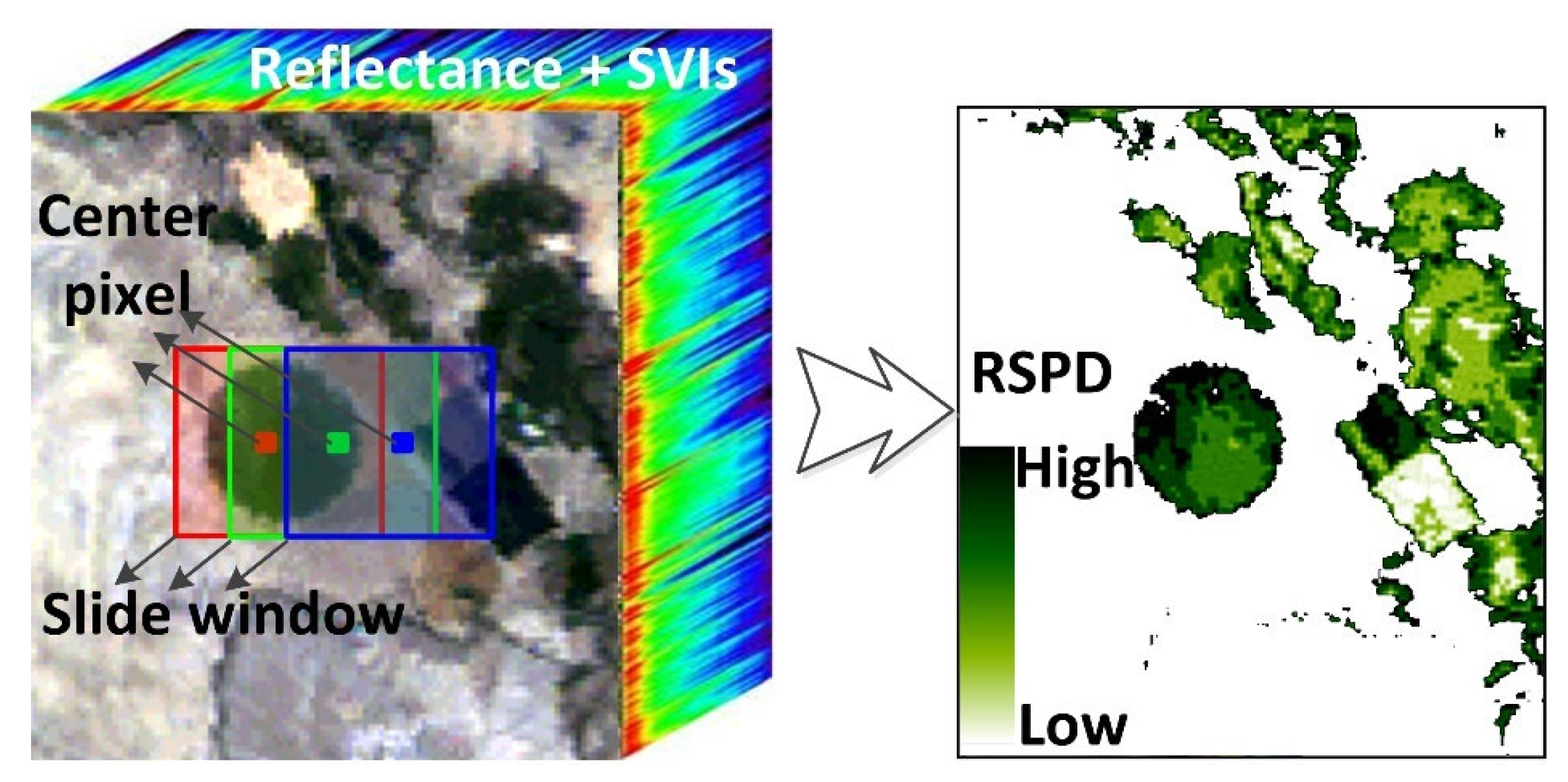
2.1. Calculating the RSPD

Figure 1 shows the conceptual graph of the method for calculating the suggested RSPD. Firstly, the RSPD is expected to be implemented in a local area which can be a plot or study area. Supposing there is a sliding window on the image and the center of the sliding window is vegetated pixel, all vegetated pixels in the sliding window are taken as input for the method and one value of RSPD will be obtained from the method as output. The output value is then assigned to the center pixel of the sliding window, which is considered a measure of plant diversity within the sliding window area.

In addition, the suggested RSPD is expected to operate on a composition of varied reflectance bands and spectral vegetation indices (SVIs). The reflectance has a fixed data range between 0 and 1, while the data range of SVI may vary with the specific calculation technique. In this study, a technique such as the normalized difference vegetation index (NDVI) is suggested to calculate the SVI because it has a fixed range from −1 to +1 and the NDVI has been successfully used in reflecting plant biomass and productivity. The SVI can be expressed as:

$$\mathrm{SVI}=\frac{{\rho }_{b1}-{\rho }_{b2}}{{\rho }_{b1}+{\rho }_{b2}},$$

(1)

where ${\rho }_{b1}$ and ${\rho }_{b2}$ are reflectance at the bands of b1 and b2, respectively. The SVI has a theoretical range between − 1 and 1. In order to keep with the data range of reflectance, the SVI can be normalized by the equation (SVI + 1)/2. Resultantly, varied reflectance bands and normalized SVI data were combined into a multi-band image file. For this file, each vegetated pixel can be represented with a multi-dimensional vector:

$$X_i=\left[v_{i,1},v_{i,2},v_{i,3},\cdots ,v_{i,n}\right],$$

(2)

where $X_i$ is the $i$-th vegetated pixel; ν is the value at each band with a fixed data range of [0,1]; $n$ is the total number of the bands.

Assuming $X_0$ is the central vegetated pixel in a sliding window, the similarity between the other vegetated pixels and the $X_0$ can be expressed as:

$$D_i=\left|X_i-X_0\right|=\sqrt{{\displaystyle {\sum }_{j=1}^n{\left(v_{i,j}-v_{0,j}\right)}^2}},$$

(3)

where $D_i$ is a measure of similarity among varied vegetated pixels. This similarity has a theoretical maximum of $\sqrt{n}$ and a theoretical minimum of 0 because of the data range of $v$ varied from 0 to 1. It is noteworthy here that we employ the $D_i$ to determine if $X_0$ and $X_i$ belong to the same plant species. According to spectral variation hypothesis and productivity hypothesis, the smaller $D_i$ means the greater probability of belonging to the same plant species and vice versa. In order to determine the thresholds for distinguishing different species, we divide the $D_i$ uniformly from theoretical minimum to theoretical maximum into $Q$ segments. The vegetation pixels with similarity falling into the same segment is considered as belonging to the same plant species. Additionally, those falling into different segments were considered to be different plant species. Resultantly, the following equation can be used to calculate the relative abundance of each segment:

$$p_q=C\left(\frac{\left(q-1\right)\times D_{\max }}{Q}\le D<\frac{q\times D_{\max }}{Q}\right)/\mathrm{W},$$

(4)

where $p_q$ is the relative abundance of the $q$-th segment, that is, the proportion of each segment in the window to the total number of pixels in the window; $Q$ is the number of segments (100 in this study); $D_{\max }=\sqrt{n}$; $\frac{D_{\max }}{Q}$ is the length of each segment; $C$ is a function returning the number of vegetated pixels whose similarity $D$ follows the condition that $\frac{\left(q-1\right)\times D_{\max }}{Q}\le D<\frac{q\times D_{\max }}{Q}$; and $\mathrm{W}$ is the total number of vegetated pixels in the sliding window. Finally, the following equation was used to calculate the remote sensing index of plant diversity for this sliding window referring to the Shannon entropy:

$$\mathrm{RSPD}=\frac{-{\displaystyle {\sum }_{q=1}^Q{p}_q\times }\ln \left(p_q\right)}{\ln \left(Q\right)},$$

(5)

where ln( ) is the natural logarithm. The value of RSPD has a fixed range between 0 and 1, where the greater value indicates the greater plant diversity and vice versa.

2.2. Evaluating the RSPD

The RSPD was evaluated by comparing with the typical CV method, which can be expressed as:

$$\mathrm{CV}=\frac{{\displaystyle {\sum }_{\lambda =1}^{\Delta }\left(\frac{std\left({\rho }_{\lambda }\right)}{mean\left({\rho }_{\lambda }\right)}\right)}}{\Delta },$$

(6)

where ${\rho }_{\lambda }$ is spectral reflectance at the band of $\lambda$, $\Delta$ is the total number of spectral bands, $std\left(\right)$ is the function to obtain standard deviation, and $mean\left(\right)$ is the function to obtain average value.

Additionally, we also used a non-supervised classification method to identify as many different plant species as possible. Common unsupervised classification methods include the K-means clustering analysis method and ISODATA. We mainly used the K-means clustering analysis method and set the number of classes to 30 and the maximum iteration to 20. The classification results indicate the plant type of each vegetated pixel. Therefore, we can obtain the richness and abundances of plant species from the classification result. Consequently, the Shannon diversity index (ShDI) and Simpson diversity index (SiDI) were calculated from the classification results using the same method of the sliding window as the RSPD, and the window size was 3 × 3:

$$\{\begin{array}{l}\mathrm{ShDI}=-{\displaystyle {\sum }_{m=1}^M{p}_m\times }\ln \left(p_m\right)\\ \mathrm{SiDI}=1-{\displaystyle {\sum }_{m=1}^M{p}_m^2}\end{array},$$

(7)

where P_m is the ratio of pixel numbers with vegetation type m to the total vegetated pixel numbers within the sliding window.

Using ShDI and SiDI as reference, two quantitative indicators were selected to evaluate the performance of the RSPD. One of them was the Pearson correlation coefficient, which ranges from −1 to 1. The larger the correlation coefficient is, the better the RSPD performance is. Another indicator was image texture difference (ITD), which is defined following the equation provided in Sun et al. (2015) [38]. The ITD is dimensionless, where smaller values correspond to an increasingly similar spatially distributed RSPD and ShDI/SiDI.

$$\mathrm{ITD}=\frac{{\displaystyle \sum _{j=1}^m\sqrt{{\displaystyle \sum _{i=1}^n{(T_{i,j}^{\mathrm{I}}-T_{i,j}^{\mathrm{II}})}^2/n}}}}{m},$$

(8)

where $T_{i,j}^{\mathrm{I}}$ and $T_{i,j}^{\mathrm{II}}$ are the normalized texture measures of the RSPD and ShDI/SiDI images, respectively, where $i$ varies from 1 to $n$ indicating pixel location, and $j$ varies from 1 to $m$ representing various image texture measures. Eight texture measures were computed in this study, including mean, variance, homogeneity, contrast, dissimilarity, entropy, second moment, and correlation.

3. Study Materials and Cases

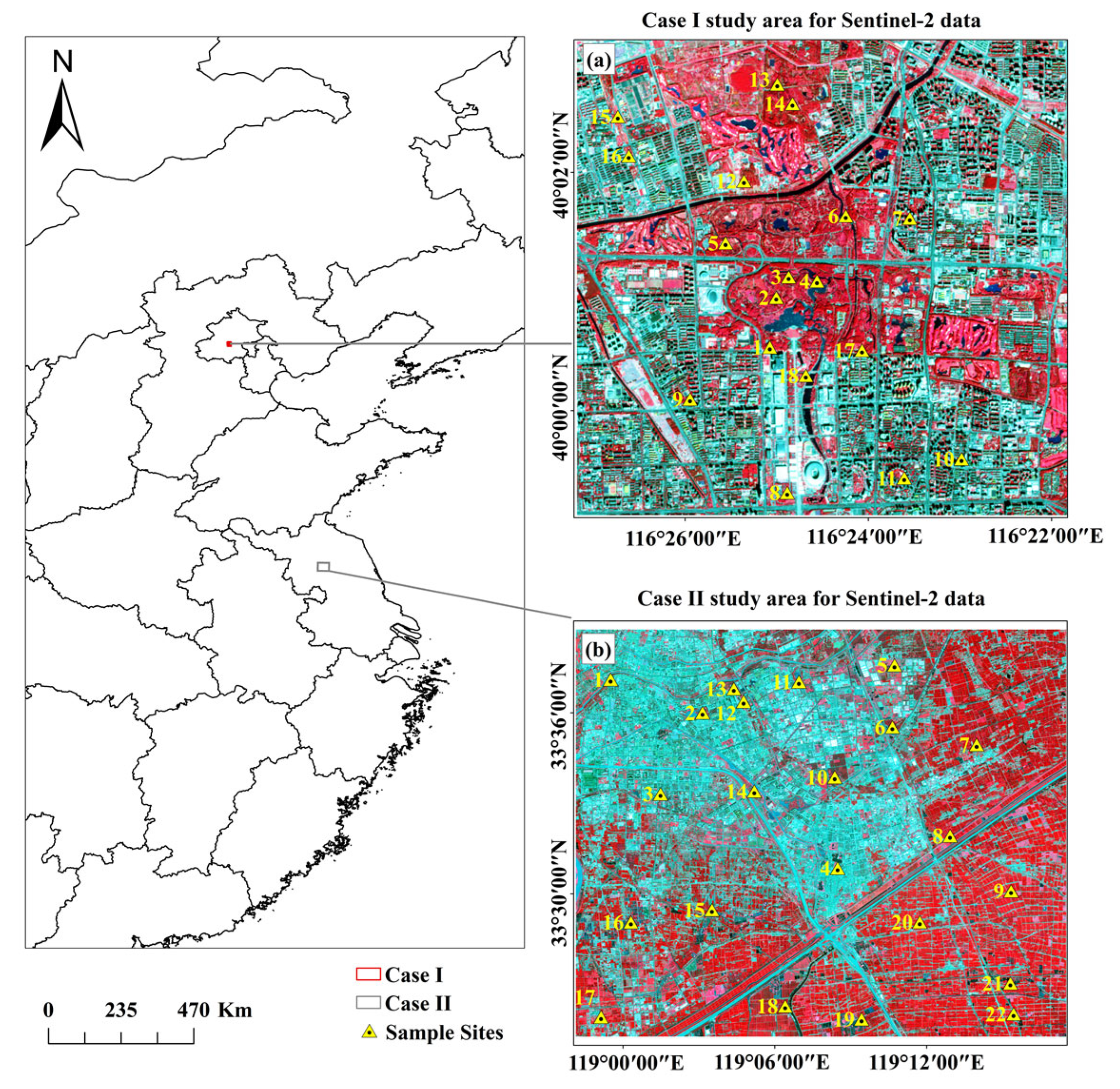
3.1. Study Cases

Two cases were selected in this study; where Case I was located in the megacity, Beijing and Case II was located in part of Huai’an, China. Figure 2 illustrates the spatial distribution of the two study areas. Case I was the area around the Beijing Olympic Forest Park, which covers an area of about 680 hectares, with more than 550,000 trees and shrubs, 280 plant varieties, and a green coverage ratio of about 95.61%. Case II was located in the northeast of the Qingjiangpu District of Huai’an City. The forest coverage rate of Huai’an City is 18.2%. There are 90,700 hectares of forest land and 380,000 hectares of farmland–forest networks in the city, and the forest network rate is 95.9%. Among them, the forest resources are mainly artificial forest and natural forest, and the tree species resources are relatively rich. There are 79 families of woody plants, 410 species of 179 genera, including 328 species of trees, 65 species of shrubs and 17 species of vines in Huai’an. Vegetation in the study area is mainly distributed in the southeast, mainly in farmland and forest network, and in the northwest, mainly in buildings.

3.2. Sentinel-2 Data

The remote sensing data from Copernicus Sentinel-2 mission were used in this study. Specifically, the optical data from MultiSpectral Instrument (MSI), the main instrument of the Sentinel-2 mission, was employed. Images include data on 28 August 2016, 5 September 2018, and 19 September 2020 in Case I, and data on 26 July 2016, 9 September 2018, and 3 September 2020 in Case II.

There are thirteen spectral bands provided by the MSI within the wavelength region from visible to short-wave infrared band. Moreover, there are three spatial resolutions for different spectral bands: 10 m, 20 m, and 60 m.

Table 1. Spectral bands for the Sentinel-2 sensors (S2A&S2B).

Band Number	S2A		S2B		Spatial Resolution (m)
	Central Wavelength (nm)	Bandwidth (nm)	Central Wavelength (nm)	Bandwidth (nm)
1	443.9	27	442.3	45	60
2	496.6	98	492.1	98	10
3	560	45	559	46	10
4	664.5	38	665	39	10
5	703.9	19	703.8	20	20
6	740.2	18	739.1	18	20
7	782.5	28	779.7	28	20
8	835.1	145	833	133	10
8a	864.8	33	864	32	20
9	945	26	943.2	27	60
10	1373.5	75	1376.9	76	60
11	1613.7	143	1610.4	141	20
12	2202.4	242	2185.7	238	20

shows the parameters of each band of Sentinel-2 data. The bands with spatial resolutions of 60 m were excluded in this study because of their coarse resolution. The collected products are at the level of Level-1C which is top-of-atmosphere reflectance in cartographic geometry. Therefore, we first used Sen2cor to implement radiation calibration and atmospheric correction on Level-1C products to generate bottom-of-atmosphere reflectance data (i.e., Level-2A). Secondly, in order to unify the spatial resolution, we re-sampled the spectral bands to a 10 m resolution using the Sentinel series data processing software Sentinel Application Platform (SNAP), provided by ESA. The SNAP is the common architecture of all Sentinel Toolboxes and SMOS Toolbox, which can process Sentinel series data, Landsat series data, SPOT series data and SAR data such as geometric correction, radiometric calibration, filtering, clipping, mosaic, etc. Based on the Level-2A data, we computed the fractional vegetation coverage (FVC) with the tools in SNAP software. In order to implement the RSPD method, non-vegetated pixels should be masked. We identified the vegetated pixels by the conditions that it is a vegetation type classified by the Sen2Cor’s built-in scene classification algorithm [35] and its FVC is greater than 50%.

According to the spectral bands of Sentinel-2 MSI, we calculated the following spectral vegetation indices:

$$\{\begin{array}{l}\mathrm{NDVI}=\left({\rho }_{b8}-{\rho }_{b4}\right)/\left({\rho }_{b8}+{\rho }_{b4}\right)\\ {\mathrm{NDVI}}_{RE1}=\left({\rho }_{b5}-{\rho }_{b4}\right)/\left({\rho }_{b5}+{\rho }_{b4}\right)\\ {\mathrm{NDVI}}_{RE2}=\left({\rho }_{b6}-{\rho }_{b4}\right)/\left({\rho }_{b6}+{\rho }_{b4}\right)\\ {\mathrm{NDVI}}_{RE3}=\left({\rho }_{b7}-{\rho }_{b4}\right)/\left({\rho }_{b7}+{\rho }_{b4}\right)\\ {\mathrm{NDVI}}_{RE4}=\left({\rho }_{b8a}-{\rho }_{b4}\right)/\left({\rho }_{b8a}+{\rho }_{b4}\right)\\ {\mathrm{NDII}}_1=\left({\rho }_{b8}-{\rho }_{b11}\right)/\left({\rho }_{b8}+{\rho }_{b11}\right)\\ {\mathrm{NDII}}_2=\left({\rho }_{b8}-{\rho }_{b12}\right)/\left({\rho }_{b8}+{\rho }_{b12}\right)\end{array},$$

(9)

where $\rho$ represents reflectance, $b4$~$b12$ represent spectral bands of Sentinel-2 MSI. Finally, 10 reflectance bands (b2, b3, b4, b5, b6, b7, b8, b8a, b11, b12) and the above 7 spectral vegetation indices were combined into a file with 17 bands to calculate the suggested RSPD. The unsupervised classification was also conducted on the 17 reflectance bands. The typical CV method was conducted on the 10 reflectance bands according to its original meaning.

3.3. Pléiades-1 Data

Pléiades-1 high-resolution imagery was also utilized in this study. These data were acquired on 23 September 2018, and the spatial coverage was the same with Case II, as shown in Figure 2. These data have a rich texture structure and qualified quality without cloud and snow. Pléiades is the first European very-high-resolution (VHR) satellite system that provides sun synchronous imagery from an orbit height of 674 km with a swath width of 20 km and a daily revisit capability. The sensor can reach a ground resolution of 0.5 m in panchromatic mode and 2 m in multi-spectral mode in the vertical direction. The Pléiades consists of five channels: Panchromatic (470–830 nm), Blue (430–550 nm), Green (500–620 nm), Red (590–710 nm), and Near-infrared (740–940 nm). Since these data have higher spatial resolution than the Sentinel-2, they were utilized as one of the references to evaluate the suggested RSPD.

4. Results

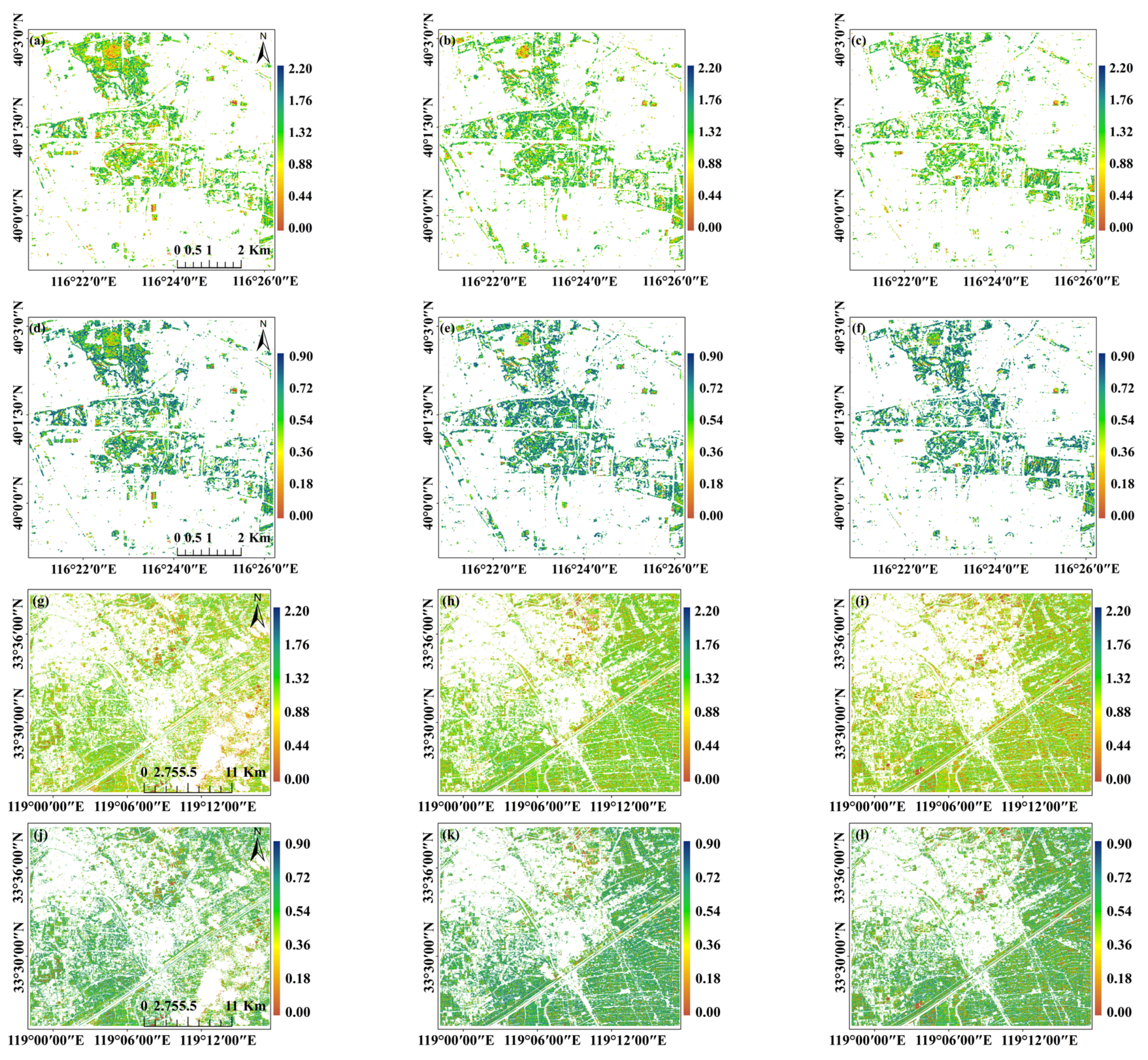
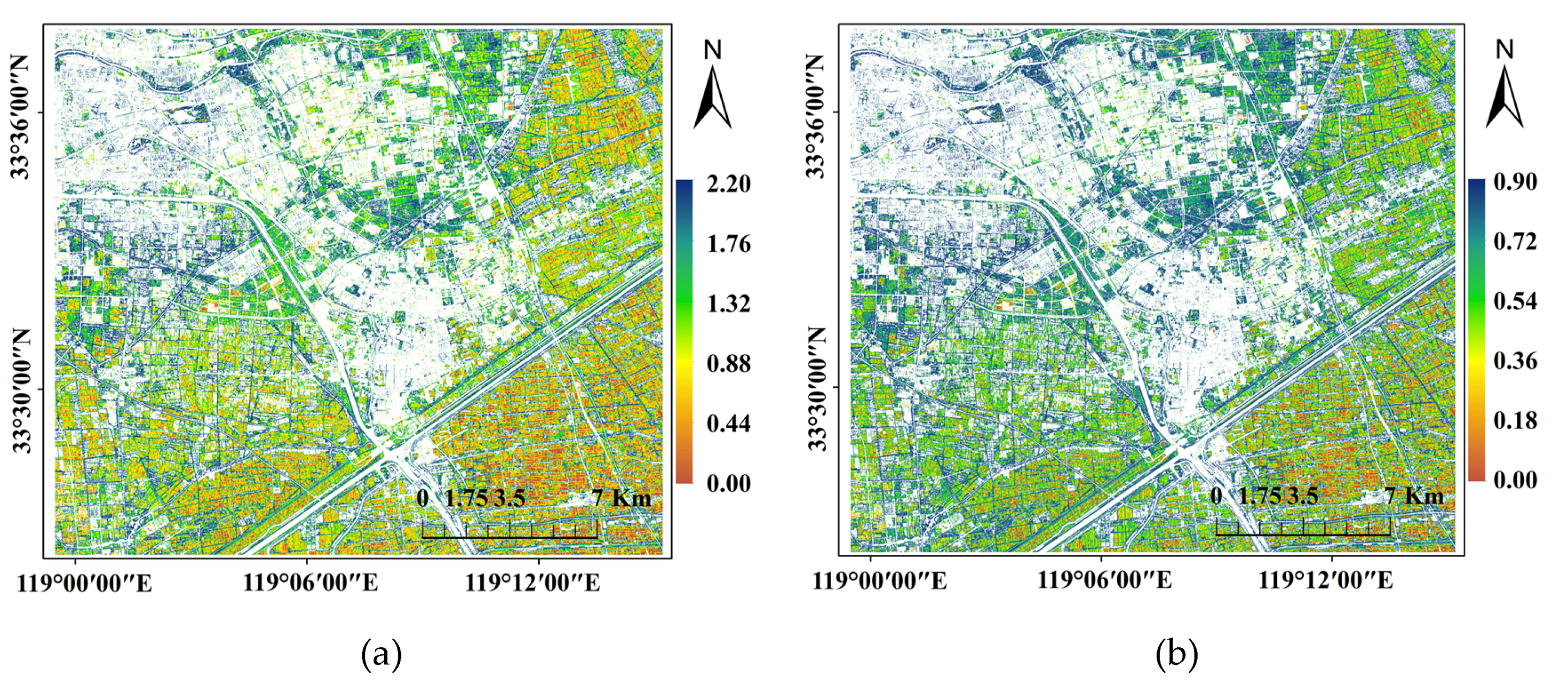
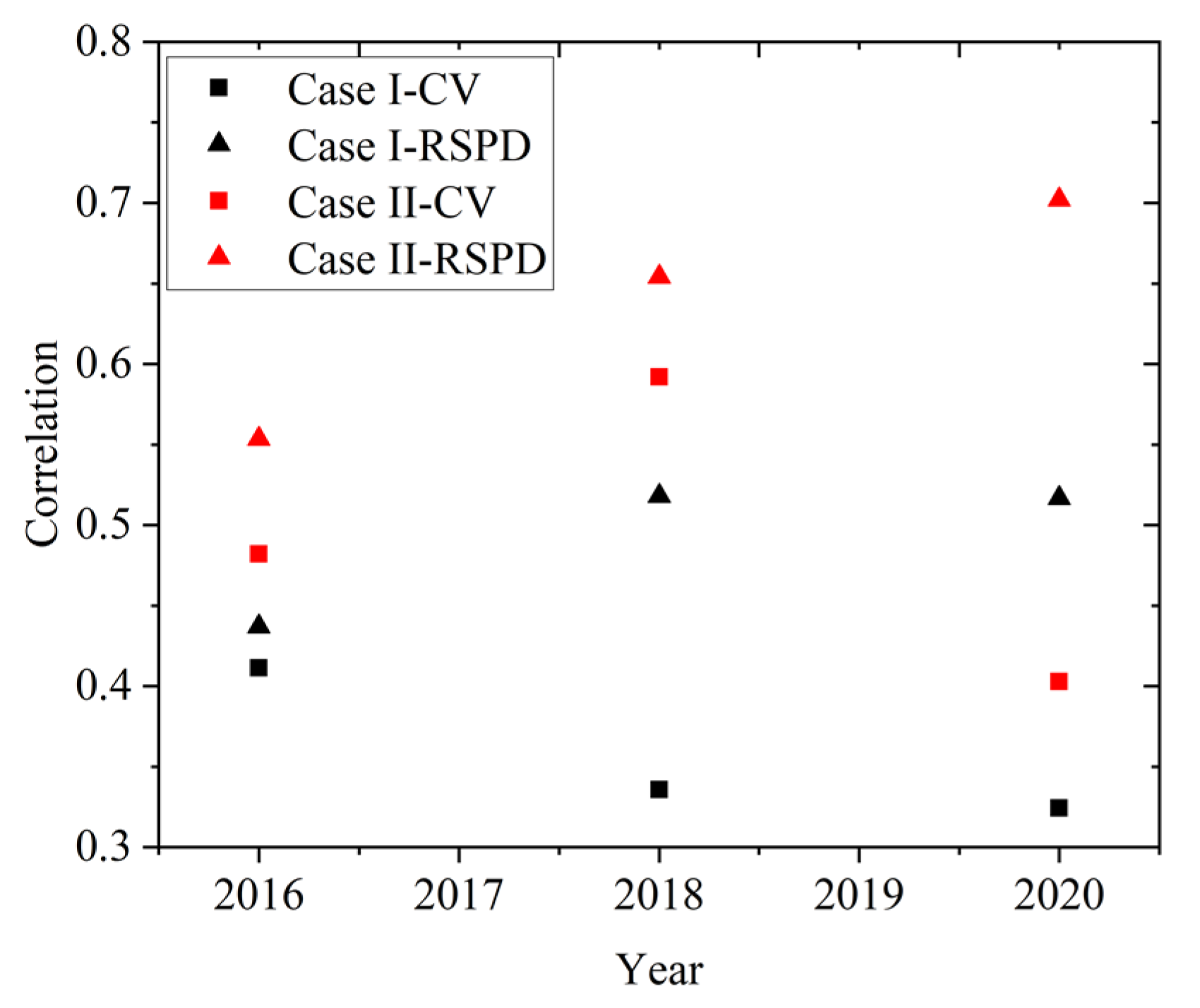
4.1. Spatiotemporal Comparisons between RSPD and CV

Figure 3 shows the results of the RSPD and CV in the Case I and Case II area based on Sentinel-2 data. The first line (a), (b), and (c) are the RSPD results of Case I on August 28, 2016, September 5, 2018, and September 19, 2020, respectively. The second line (d), (e), and (f) are the CV results of Case I on those days. The greater value of the RSPD and CV indicates the greater plant diversity, and vice versa. It can be seen that the spatial distributions of the RSPD and CV are basically consistent in Case I. The central and northern regions have higher plant diversity, which are mainly with medium and high fractional vegetation coverage. The other areas are surrounded by built-up areas, which have lower plant diversity. Figure 3g–l show the distribution of the RSPD and CV in Case II on different days. Once again, the distributions of the RSPD and CV are basically consistent with each other. The RSPD and CV both illustrate that the northwest of Case II has lower plant diversity, while a higher plant diversity is in the southeast of this area.

We conducted statistical analysis on the maximum and mean values of the RSPD and CV, respectively.

Table 2. Statistical analysis of RSPD and CV in Case I.

Case I	Min		Max		Mean
	RSPD	CV	RSPD	CV	RSPD	CV
2016	0	0.001358	0.443673	0.285537	0.215822	0.061429
2018	0	0.001528	0.477121	0.493477	0.237009	0.086106
2020	0	0.003064	0.477121	0.504260	0.253524	0.096511

and

Table 3. Statistical analysis of RSPD and CV in Case II.

Case II	Min		Max		Mean
	RSPD	CV	RSPD	CV	RSPD	CV
2016	0	0.002980	0.477121	0.686903	0.210889	0.083789
2018	0	0.001722	0.477121	0.481739	0.219088	0.092678
2020	0	0.004737	0.477121	0.449763	0.183124	0.078497

are the statistical information of the two study areas, respectively. Additionally, the temporal variations of the RSPD and CV are shown in Figure 4. Overall, the Case I study area shows a trend of an increase in plant biodiversity from 2016 to 2020. The plant diversity in the Case II region shows a tiny upward trend from 2016 to 2018, but a slight downward trend from 2018 to 2020. The variation trend of the RSPD and CV are also basically the same.

In summary, the RSPD and CV are basically consistent with each other in depicting the spatial and temporal variation of plant diversity.

4.2. Evaluating RSPD and CV with Classification Results by Sentinel-2 Data

Figure 5 shows the spatial distribution of ShDI and SiDI for Case I and Case II. First of all, the distribution results are consistent with the spatial patterns and variation trend of the RSPD. Additionally, Figure 6a,b present the correlation coefficients between the ShDI/SiDI and RSPD/CV. The correlation coefficients between the RSPD and ShDI/SiDI are greater than 0.9 with p-value = 0.01.

Figure 6c,d show the ITD between the RSPD/CV and the ShDI/SiDI at various times during 2016–2020. The horizontal axis represents the temporal variation, and the vertical axis indicates the value of the ITD. A greater ITD corresponds to a greater RSPD/CV −ShDI/SiDI spatially distributed difference. It can be seen from Figure 6 that the ITD value between the RSPD and ShDI/SiDI is generally smaller, while the ITD value between the CV and ShDI/SiDI is generally bigger. These results indicate that the diversity indicated by the RSPD is in good agreement with the spatial distribution pattern of ShDI/SiDI. Moreover, the RSPD results outperform the CV in all cases and study periods.

4.3. Evaluating RSPD and CV with Classification Results by Pléiades-1 Data

We also calculated the ShDI and SIDI using high-resolution Pléiades-1 data over the Case II area in 2018. Figure 7 shows the spatial distribution of the ShDI and SiDI results. It can be seen that the spatial patterns are consistent with the distribution of the RSPD in 2018.

Furtherly, we compared the correlation coefficient and ITD between the RSPD/CV based on Sentinel-2 data and ShDI/SiDI based on Pléiades-1 data. Since they have different spatial resolutions, we simply disaggregated the coarse-resolution data into the high-resolution with nearest neighbor resampling. Comparison results are shown in Figure 8. The correlation coefficients between the RSPD/CV and ShDI/SiDI are greater than 0.6 at a significant level of 0.05. ITDs are all less than 0.35. Once again, the RSPD outperforms the CV, as compared with ShDI/SiDI based on Pléiades-1 data.

In summary, the suggested RSPD is basically consistent with the classical CV method. However, the overall performance of the RSPD is better than that of the CV, as compared in spatial details and with vegetation classification results using similar and higher-resolution images.

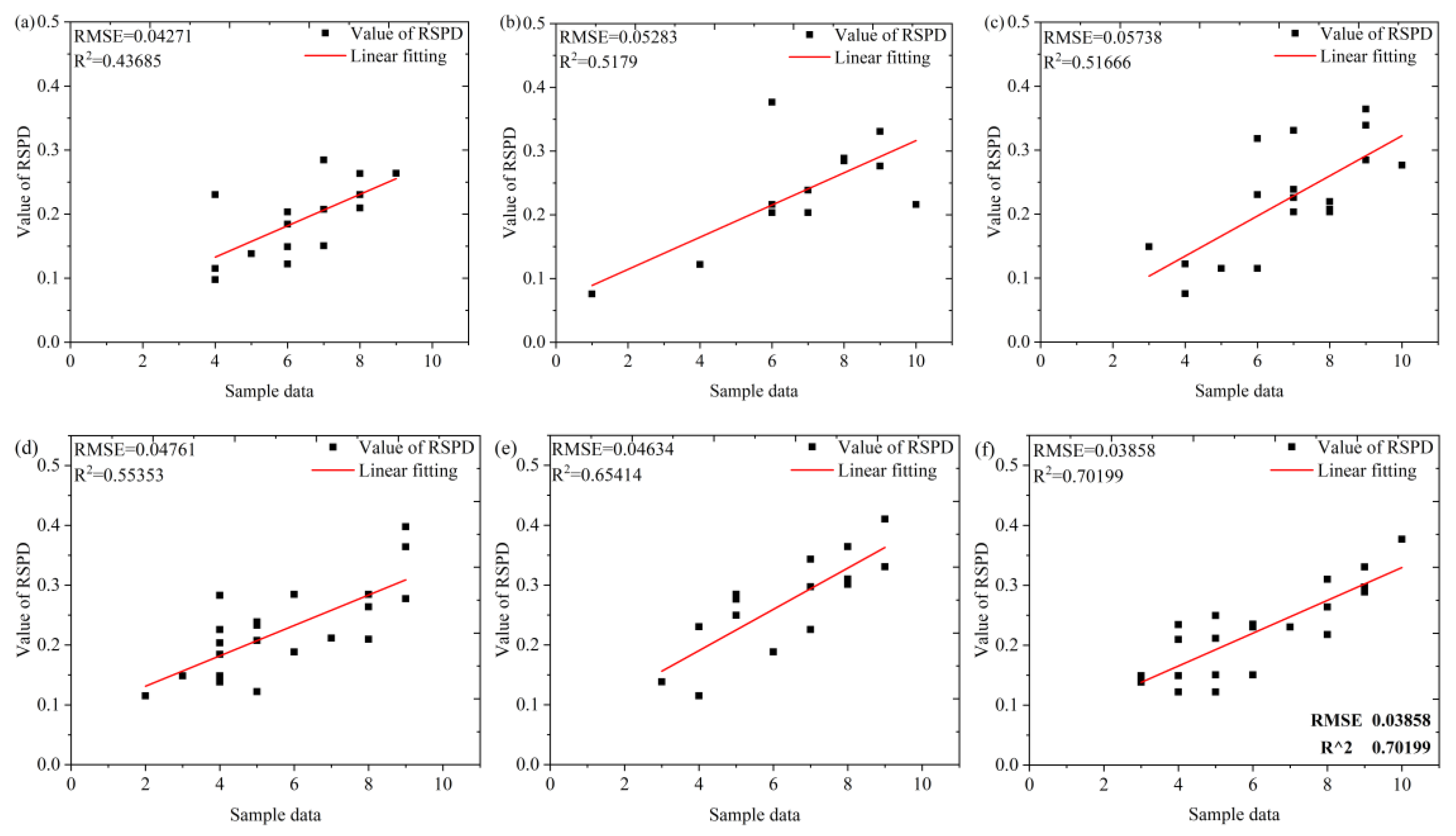
4.4. Evaluating RSPD with Visual Interpretation of Google Earth Image

In addition to the aforementioned evaluations of the RSPD with the CV, ShDI, and SiDI with similar resolution and higher resolution images. Here, we present another evaluation with visual interpretations of Google Earth image.

Firstly, we compared the RSPD and CV in 2020 with Google Earth image and in situ pictures through selecting three targets of forest, forest–grassland mixture, and grassland in Case I as shown in Figure 9. We used the visual interpretation method to compare the distribution of the RSPD/CV and Google Earth images at the targets to judge the performance of the RSPD.

As can be seen from the Google Earth images and in situ pictures, target 1 is located in the forest, mainly distributed with a large number of shrubs, trees and herbs, with rich species and the highest diversity. Target 2 is located in forest–grassland mixture and has less species diversity than the forest target. Target 3 is grassland with single vegetation type and has the lowest species diversity. Figure 9a–f demonstrate that the results of the RSPD and CV at the three targets are consistent with the above visual interpretations, although there are subtle differences between the RSPD and CV.

Secondly, 40 samples in 30m*30m were selected from Google Earth, which include 18 in the Beijing Olympic Forest Park and surrounding areas, and 22 in Huai’an City. The distribution of sample sites is shown in Figure 2. According to the satellite images and panoramas of Google Earth, the vegetation coverage and the number of species in each plot were estimated, and the degree of plant diversity was determined and graded. The classification results are shown in

Table 4. Plant diversity grade of sample sites.

Sample Sites	Case I			Case II
	2016	2018	2020	2016	2018	2020
1	9	10	10	5	//	5
2	8	4	7	4	//	4
3	8	8	9	6	//	6
4	7	8	8	5	//	5
5	//	6	4	8	8	8
6	//	4	4	8	8	8
7	6	8	8	7	8	7
8	4	7	5	9	9	10
9	6	6	7	3	5	4
10	5	//	7	4	//	3
11	7	7	9	4	//	4
12	7	9	9	5	//	5
13	4	//	6	9	9	8
14	6	//	6	4	5	3
15	4	1	3	8	7	9
16	//	//	7	5	7	6
17	8	9	8	6	4	6
18	6	6	6	2	3	3
19	//	//	//	8	7	9
20	//	//	//	4	5	5
21	//	//	//	4	4	4
22	//	//	//	9	6	9

.

Figure 10 show the scatter plots between the RSPD and the level of plant diversity at sample plots in Case I and Case II. The results show that there is a significant correlation between the RSPD and the plant diversity grade of sample sites, with the determination coefficient ranging from 0.4 to 0.55 and 0.55 to 0.75 in Case I and Case II. The results show that the RSDP is effective in describing the plant diversity from the perspective of visual interpretation.

In addition, three sample points were selected in Case I and Case II, respectively. By comparing the 2016–2020 RSPD results with the time variation trend of the sample data, the performance of the RSPD was also evaluated from the time trend. The time variation results are shown in Figure 11, which indicates that the RSPD and sample data have basically the same changing trend in time series.

5. Discussion

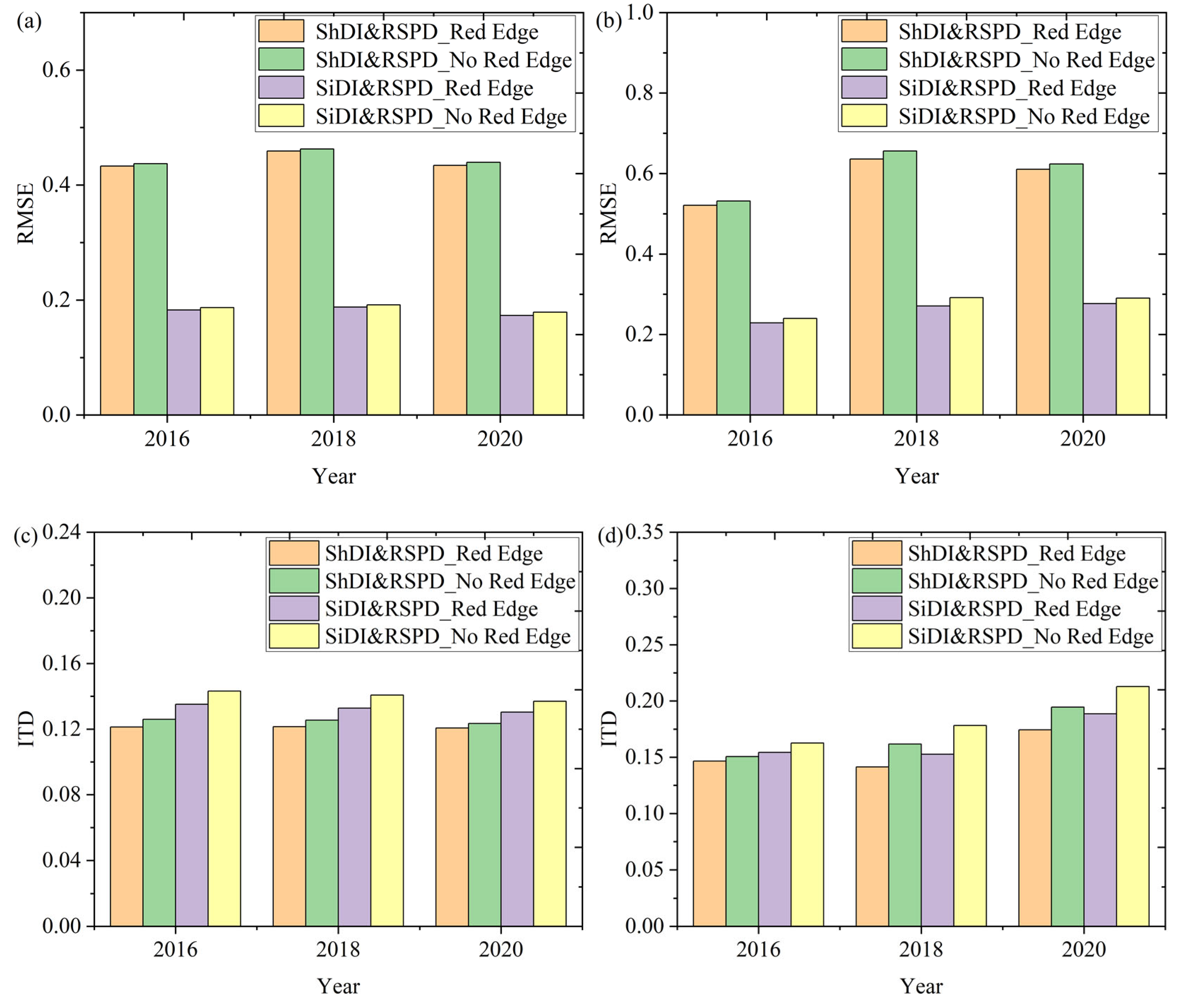
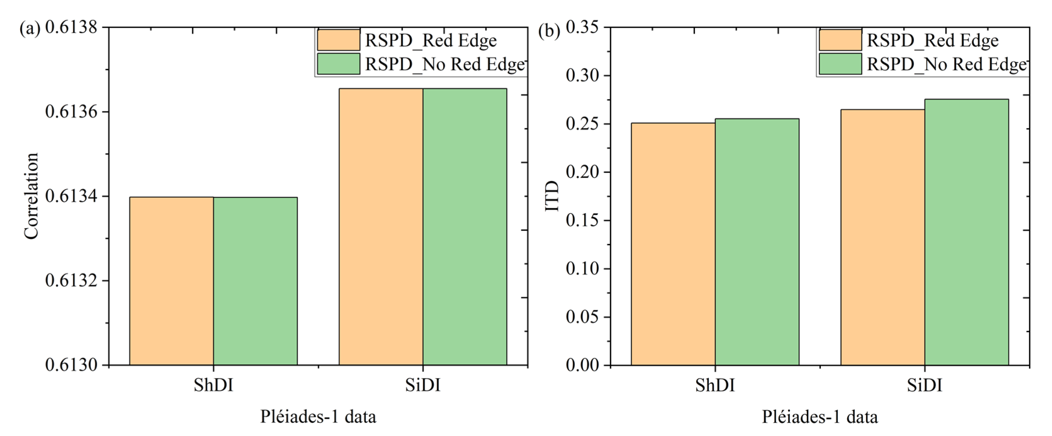
5.1. The Influence of Red-Edge Bands on RSPD

The suggested RSPD in this study is expected to be applied in other satellites not just for Sentinel-2 satellite. One striking feature of Sentinel-2 is in the multiple red-edge bands, which are important spectrum bands to reflect the biophysical status of vegetation. However, these electromagnetic wave bands are not deployed in many other optical satellites. In order to evaluate the influence of red-edge bands on the performance of the RSPD, we analyzed the difference between the RSPD models constructed with and without considering the red-edge bands. Root mean square error (RMSE) and ITD were used to evaluate the difference, and the results are illustrated in Figure 13. In Case I, the RMSE of the RSPD without considering the red-edge is between 0.43 and 0.47, as compared with the ShDI, and between 0.17 and 0.20, as compared with the SiDI. Correspondingly, the RMSE of the RSPD with red-edge is between 0.43 and 0.46 with the ShDI and 0.17 and 0.19 with the SIDI. In Case II, without considering the red-edge, the RMSE of the RSPD is between 0.53 and 0.66 for the ShDI and between 0.23 and 0.30 for the SiDI. In the case of with red-edge, the RMSE of the RSPD is between 0.52 and 0.64 with the ShDI and 0.22 and 0.28 with the SiDI. The results indicate that the difference between that with and without red-edge bands is little, although red-edge bands do help in reducing the difference.

Figure 13c,d show the ITD between the RSPD and ShDI/SiDI with or without red-edge bands at different times from 2016 to 2020. The horizontal axis represents the temporal variation, and the vertical axis indicates the value of the ITD. As can be seen from Figure 13, the ITD value between the RSPD and ShDI/SiDI in the case of red-edge is generally small, while the ITD value between the RSPD and ShDI/SiDI in the case of no red-edge is generally high. In addition, the effect of red-edge bands was also evaluated by Pléiades data-derived ShDI/SiDI. The evaluation results are shown in Figure 14. The correlation between the two RSPDs is basically equal, and the ITD of the RSPD with red-edge bands is a little lower than that without red-edge bands.

In summary, the RMSE and ITD of the RSPD with the red-edge bands are lower than that without the red-edge bands, indicating that the red-edge bands do help in promoting the performance of the RSPD. However, the difference is not very significant, as demonstrated in our study. Thus, we believe that the suggested RSPD can be applied in other optical satellites, not just for Sentinel-2 satellite.

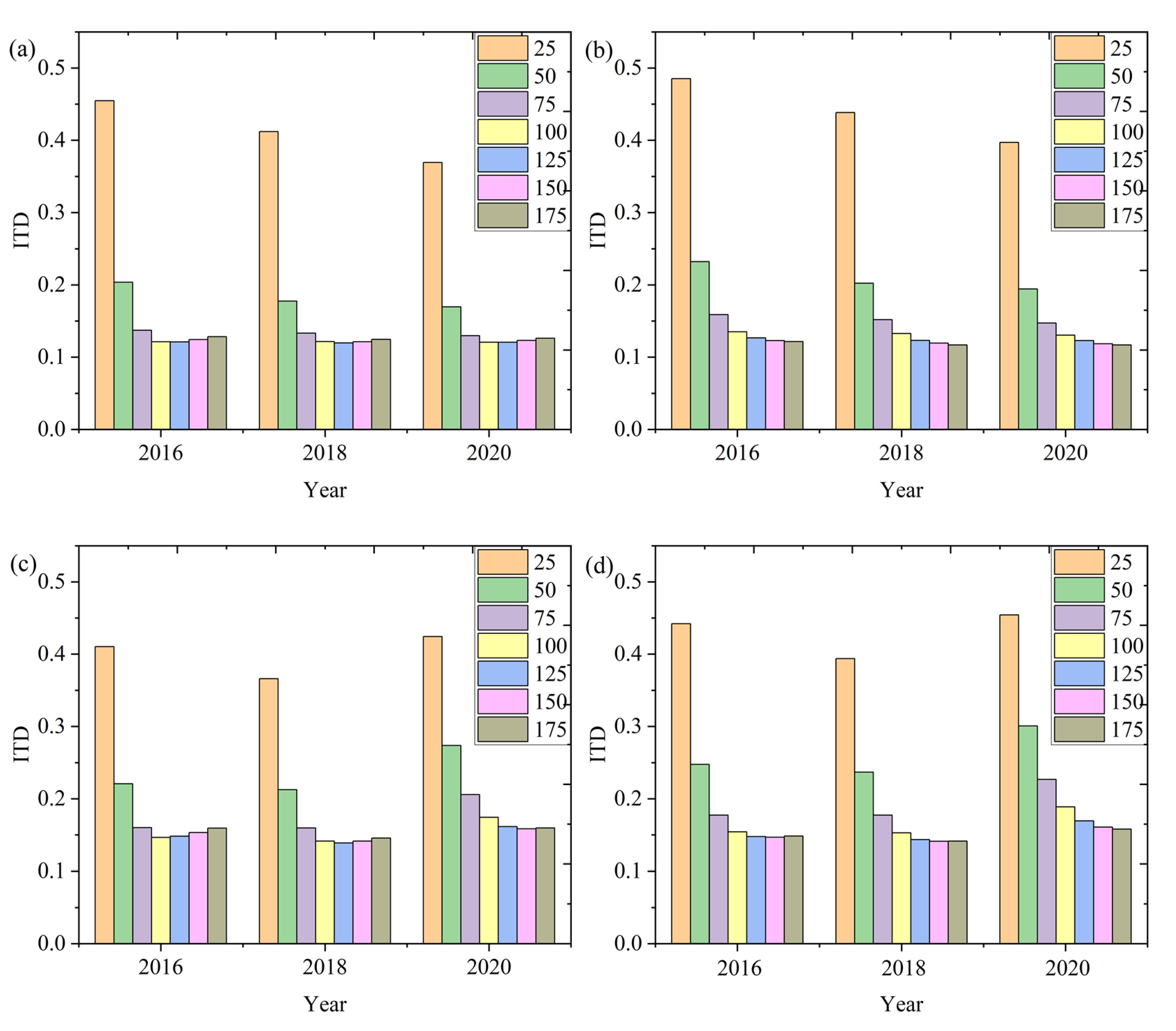
5.2. The Influence of Segment Number on RSPD

In the calculation of RSPD, the number of segments ($Q$) in Equation (4) was set as 100 according to comprehensive experiment analysis. To investigate the influence of $Q$ on the RSPD, we calculated the RSPD with different numbers of $Q$, varying between 25 and 175 in the study areas, Case I and Case II, respectively. The ITD consistency analysis between the RSPD and ShDI/SiDI was carried out to determine the appropriate $Q$. Figure 15 shows the ITD results between the RSPD and ShDI/SiDI. As can be seen from the figure, when the $Q$ changed from 25 to 75, the ITD decreased significantly, implying that the performance of the RSPD would be promoted with the increasement of $Q$. However, when the $Q$ changed from 100 to 175, there was very little variation in the ITD, implying that the effect of promotion by increasing the $Q$ is limited or convergent. Too large a value of the $Q$ would increase burden on the calculation of the RSPD. Consequently, it is appropriate to set $Q$ as 100 in this study.

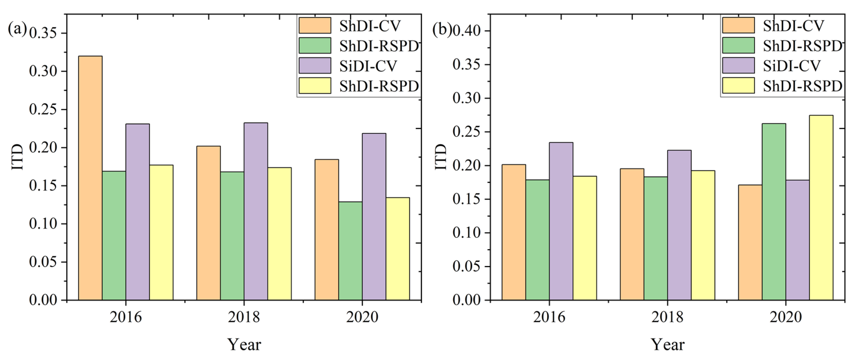
5.3. Different Unsupervised Classification Methods on Evaluating RSPD

In the above-mentioned evaluation of the RSPD with classification results, we mainly used the K-means clustering analysis method. In order to analyze the influence of different unsupervised classification methods on evaluating the RSPD, we also adopted the ISODATA unsupervised classification method, whose parameter settings are the same as the K-means clustering analysis method. Figure 16 shows the ITD between the ShDI/SiDI based on the ISODATA method and the RSPD/CV. It can be seen that the ITD is lower for the comparisons between the RSPD and ShDI/SiDI, while it is higher for the comparisons between the CV and ShDI/SiDI. This phenomenon is consistent with that by the K-means method, as shown in Figure 6. The results demonstrate that no matter which unsupervised classification method is used for evaluation, the performance of the RSPD is better than that of the CV.

5.4. Applicability and Prospects of the RSPD

At present, biodiversity and ecosystem conservation have become hot issues of global concern. Several international treaties have thus been created, such as the United Nations Convention on Biological Diversity, the United Nations Framework Convention on Climate Change, and the Paris Agreement. In the face of global environmental risks and challenges, the conservation of biodiversity has become increasingly urgent. In order to deal with the loss of biological diversity, many biologists, ecologists and other relevant researchers are committed to studying the key issues in biological diversity as well as in plant diversity, such as evaluating the extinction rate and understanding the mechanism of biodiversity loss. Among them, the remote sensing of plant diversity plays a significant role in providing large-scale, long-term, and spatial continuous monitoring data.

The main contribution of this study is constructing a new remote sensing index of plant diversity, i.e., the RSPD. It has several advantages as compared with previous indices.

• The RSPD circumvents the drawbacks of the CV. First, the RSPD has a fixed range of values between 0 and 1, which is conducive to dynamically monitoring plant diversity. However, the CV can be less than 1 for low variance distribution, and greater than 1 for high variance distribution. In other words, there is no fixed range for the CV. Besides, the CV value is very susceptible to small changes in the ${\mu }_i$ and it would approach infinity when the ${\mu }_i$ is close to zero. In contrast, the RSPD can circumvent the limitations of ${\mu }_i$ in CV.
• The RSPD is designed to be implemented on a spectral measurement data set synthesized by spectral reflectance and various spectral vegetation indices (e.g., vegetation greenness index, vegetation moisture index, red-edge vegetation index). The spectral vegetation indices can represent the productivity of plant to some extent. The multi-band vegetation reflectance can describe the spectrum feature of plants. Thus, the suggested RSPD combined the productivity hypothesis with the spectral variation hypothesis to monitor the plant diversity.
• Thirdly, the final calculation form of the RSPD referred to the principle of Shannon information entropy. It should be noted that plant diversity should be determined by both species’ richness and evenness. The Shannon information entropy has the ability to integrate the richness and evenness, which is inherent in its calculation formula. The well-known Shannon Diversity index is also based on the principle of Shannon information entropy. Resultantly, the suggested RSPD realized the comprehensive measurement of species richness and evenness.
• Many remote sensing-based methods for mapping plant diversity rely on a field botany survey. That is because they require a large number of field samples to train a mathematical relationship between plant diversity and remote sensing observations. However, conducting a field botany survey is usually costly, and thus has limited application potential. Actually, many areas do not have the economic and technical conditions to carry out field botanical investigation. The suggested RSPD method is a purely remotely sensed index, which means that it can evaluate and monitor the plant diversity independent of field survey. In other words, the RSPD facilitates large-scale and long time series monitoring of plant diversity.
• The proposed RSPD method is not only applicable for Sentinel-2 data. We distinguished that the multiple red-edge bands have a limited promotion effect on the RSPD, implying that the method can also be utilized in other optical satellites such as Landsat and SPOT. It can also be applied with hyperspectral data such as Hyperion, Chris, and the newly launched Zhuhai-1 hyperspectral satellite.

Certainly, there are some limitations that need to be solved in the future, which are not only for the RSPD but also for most remote sensing methods of plant diversity.

• Firstly, optical remote sensing usually obtains the spectral reflectance from the upper canopy. The understory species are hard to be observed because of the shielding effect. Furtherly, remote sensing has a spatial scale effect, which means that it chiefly reflects the information at the observing scale. With regard to the remote sensing of plant diversity, it can only identify the dominant species at the observing scale. Therefore, we admit that the suggested RSPD and the classical CV methods may not have the capacity to map the diversity of the entire plant community. This study only demonstrates the RSPD’s capacity to map diversity of dominant species. Additionally, due to the existence of mixed pixel, the suggested RSPD and the CV may both be sensitive to habitat heterogeneity. In this study, we have tried our best to mask the non-vegetated pixels. We think this limitation can be reduced with the increasing improvement in spatial resolution of remote sensing technology.
• Secondly, it has been described that while remote sensing indices are closely related to plant diversity, they are also influenced by important factors related to climate, ecosystem type, degree of disturbance, topography, and land cover [39,40]. Therefore, we declare that the suggested RSPD should be implemented in a time scale of a year. The annual RSPD should be the maximum RSPD during a year-long observation, especially the observation during the vegetation growing season. The maximum value composite of RSPD could reduce the effect of seasonal or meteorological variation. On the other hand, due to the expensive cost in conducting field investigating, field survey data were not utilized in this study. However, we believe that the RSPD would work better if it is properly calibrated using field observations, because we have proved that the suggested RSPD is an improvement of the existing CV through the verification with other higher-resolution data.
• The main principle of our model is to reflect plant diversity using spectral variation and productivity hypotheses. If the spectral differences of different vegetation in the ecosystem are very small or the spectra of the same species are significantly different due to environmental factors (i.e., the “different objects with the same spectra” or “same objects with different spectra”), the sensitivity of the model to plant diversity will be reduced. In addition, the sensitivity of the model will also be affected if there is no positive correlation between vegetation productivity and diversity due to the influence of local special conditions. In other words, violations of the assumptions of local conditions or ecosystem characteristics will cause our algorithm to fail. However, compared with the method of only using one hypothesis, our model integrates two hypotheses to reduce the limitations to a certain extent.

In spite of these limitations, the proposed RSPD provides an advanced tool to monitor and evaluate the changes in plant diversity and the ecological restoration quality of the ecosystem. We believe that with the development of remote sensing technology, the improvement of spatiotemporal resolution and spectral resolution will provide more possibilities for the RSPD.

6. Conclusions

In this study, a new remote sensing index of plant diversity named RSPD was suggested through combining the spectral variation hypothesis and productivity hypothesis. Specifically, the RSPD combined the multi-channel spectral reflectance and several spectral vegetation greenness, moisture, and red-edge vegetation indices with the principle of Shannon information entropy and Euclidean distance. The suggested RSPD was evaluated by comparing with the classical CV method, the Shannon and Simpson diversity indices based on vegetation classification results with similar and higher resolution images, and the visual interpretations with higher resolution Google Earth images.

The results demonstrate that: (1) the RSPD is basically consistent with the CV in spatiotemporal variation; (2) the RSPD outperforms the CV as compared with classification results with Sentinel-2 data and Pléiades-1 data; (3) the RSPD outperforms the CV as compared with visual interpretations with Google Earth images. We also analyzed the effect of red-edge bands on the RSPD. The results show that the red-edge bands can improve the performance of the RSPD, but the promotion is limited, which implying that the RSPD has wide application for other optical satellites in addition to the Sentinel-2. The suggested RSPD utilized the principle of Shannon information entropy, which can comprehensively reflect the richness and evenness of plant species, because of the inherent calculation formula. The RSPD has great potential for large-scale and long time series monitoring of plant diversity. The performance of the RSPD can be furtherly improved with the advance in the spatial–temporal–spectral resolution of remote sensing technology, as well as by combining it with field observations.

References

1. Pullaiah, T.; Bahadur, B.; Krishnamurthy, K.V. Plant Biodiversity. In Plant Biology and Biotechnology; Bahadur, B., Rajam, M.V., Sahijram, L., Krishnamurthy, K., Eds.; Springer: New Delhi, India, 2015; pp. 177–195. [Google Scholar] [CrossRef]
2. Wang, R.; Gamon, J.A. Remote sensing of terrestrial plant biodiversity. Remote Sens. Environ. 2019, 231, 111218. [Google Scholar] [CrossRef]
3. Barnosky, A.D.; Matzke, N.; Tomiya, S.; Wogan, G.O.U.; Swartz, B.; Quental, T.B.; Marshall, C.; McGuire, J.L.; Lindsey, E.L.; Maguire, K.C.; et al. Has the Earth’s sixth mass extinction already arrived? Nature 2011, 471, 51–57. [Google Scholar] [CrossRef]
4. Kerr, J.T.; Ostrovsky, M. From space to species: Ecological applications for remote sensing. Trends Ecol. Evol. 2003, 18, 299–305. [Google Scholar] [CrossRef]
5. Lengyel, S.; Kobler, A.; Kutnar, L.; Framstad, E.; Henry, P.Y.; Babij, V.; Gruber, B.; Schmeller, D.; Henle, K. A review and a framework for the integration of biodiversity monitoring at the habitat level. Biodivers. Conserv. 2008, 17, 3341–3356. [Google Scholar] [CrossRef]
6. Stoms, D.M.; Estes, J.E. A remote sensing research agenda for mapping and monitoring biodiversity. Int. J. Remote Sens. 1993, 14, 1839–1860. [Google Scholar] [CrossRef]
7. Roughgarden, J.; Running, S.W.; Matson, P.A. What does remote sensing do for ecology? Ecology 1991, 72, 1918–1922. [Google Scholar] [CrossRef]
8. Broadbent, E.N.; Asner, G.P.; Peña-Claros, M.; Palace, M.; Soriano, M. Spatial partitioning of biomass and diversity in a lowland Bolivian forest: Linking field and remote sensing measurements. For. Ecol. Manag. 2008, 255, 2602–2616. [Google Scholar] [CrossRef]
9. Faucon, M.-P.; Houben, D.; Lambers, H. Plant Functional Traits: Soil and Ecosystem Services. Trends Plant Sci. 2017, 22, 385–394. [Google Scholar] [CrossRef]
10. Kraft, N.J.B.; Godoy, O.; Levine, J.M. Plant functional traits and the multidimensional nature of species coexistence. Proc. Natl. Acad. Sci. USA 2015, 112, 797–802. [Google Scholar] [CrossRef] [Green Version]
11. Stein, A.; Gerstner, K.; Kreft, H. Environmental heterogeneity as a universal driver of species richness across taxa, biomes and spatial scales. Ecol. Lett. 2014, 17, 866–880. [Google Scholar] [CrossRef]
12. Brown, J.H. Two Decades of Homage to Santa Rosalia: Toward a General Theory of Diversity. Am. Zool. 1981, 21, 877–888. [Google Scholar] [CrossRef] [Green Version]
13. Wright, D.H. Species-energy theory: An extension of species-area theory. Oikos 1983, 41, 496–506. [Google Scholar] [CrossRef] [Green Version]
14. Foody, G.M. Mapping the richness and composition of British breeding birds from coarse spatial resolution satellite sensor imagery. Int. J. Remote Sens. 2005, 26, 3943–3956. [Google Scholar] [CrossRef]
15. Costanza, J.K.; Moody, A.; Peet, R.K. Multi-scale environmental heterogeneity as a predictor of plant species richness. Landsc. Ecol. 2011, 26, 851–864. [Google Scholar] [CrossRef]
16. Hurlbert, A.H.; Haskell, J.P. The effect of energy and seasonality on avian species richness and community composition. Am. Nat. 2003, 161, 83–97. [Google Scholar] [CrossRef]
17. Evans, K.L.; James, N.A.; Gaston, K.J. Abundance, species richness and energy availability in the North American avifauna. Glob. Ecol. Biogeogr. 2006, 15, 372–385. [Google Scholar] [CrossRef]
18. Leyequien, E.; Verrelst, J.; Slot, M.; Schaepman-Strub, G.; Heitkönig, I.M.; Skidmore, A. Capturing the fugitive: Applying remote sensing to terrestrial animal distribution and diversity. Int. J. Appl. Earth Obs. Geoinf. 2007, 9, 1–20. [Google Scholar] [CrossRef]
19. Adams, J.M.; Woodward, F.I. Patterns in tree species richness as a test of the glacial extinction hypothesis. Nature 1989, 339, 699–701. [Google Scholar] [CrossRef]
20. Luoto, M.; Kuussaari, M.; Toivonen, T. Modelling butterfly distribution based on remote sensing data. J. Biogeogr. 2002, 29, 1027–1037. [Google Scholar] [CrossRef]
21. Rocchini, D.; Balkenhol, N.; Carter, G.A.; Foody, G.M.; Gillespie, T.W.; He, K.S.; Kark, S.; Levin, N.; Lucas, K.; Luoto, M.; et al. Remotely sensed spectral heterogeneity as a proxy of species diversity: Recent advances and open challenges. Ecol. Inform. 2010, 5, 318–329. [Google Scholar] [CrossRef]
22. Palmer, M.W.; Earls, P.G.; Hoagland, B.W.; White, P.S.; Wohlgemuth, T. Quantitative tools for perfecting species lists. Environmetrics 2002, 13, 121–137. [Google Scholar] [CrossRef]
23. Ustin, S.L.; Gamon, J.A. Remote sensing of plant functional types. New Phytol. 2010, 186, 795–816. [Google Scholar] [CrossRef] [PubMed]
24. Gould, W. Remote sensing of vegetation, plant species richness, and regional biodiversity hotspots. Ecol. Appl. 2000, 10, 1861–1870. [Google Scholar] [CrossRef]
25. Levin, N.; Shmida, A.; Levanoni, O.; Tamari, H.; Kark, S. Predicting mountain plant richness and rarity from space using satellite-derived vegetation indices. Divers. Distrib. 2007, 13, 692–703. [Google Scholar] [CrossRef]
26. Carlson, K.M.; Asner, G.P.; Hughes, R.F.; Ostertag, R.; Martin, R.E. Hyperspectral remote sensing of canopy biodiversity in Hawaiian lowland rainforests. Ecosystems 2007, 10, 536–549. [Google Scholar] [CrossRef]
27. Rocchini, D. Effects of spatial and spectral resolution in estimating ecosystem α-diversity by satellite imagery. Remote Sens. Environ. 2007, 111, 423–434. [Google Scholar] [CrossRef]
28. Foody, G.M.; Cutler, M.E. Mapping the species richness and composition of tropical forests from remotely sensed data with neural networks. Ecol. Model. 2006, 195, 37–42. [Google Scholar] [CrossRef] [Green Version]
29. Gillespie, T.W. Predicting Woody-Plant Species Richness in Tropical Dry Forests: A Case Study from South Florida, USA. Ecol. Appl. 2005, 15, 27–37. [Google Scholar] [CrossRef]
30. Rocchini, D.; McGlinn, D.; Ricotta, C.; Neteler, M.; Wohlgemuth, T. Landscape complexity and spatial scale influence the relationship between remotely sensed spectral diversity and survey-based plant species richness. J. Veg. Sci. 2011, 22, 688–698. [Google Scholar] [CrossRef]
31. Paz-Kagan, T.; Caras, T.; Herrmann, I.; Shachak, M.; Karnieli, A. Multiscale mapping of species diversity under changed land use using imaging spectroscopy. Ecol. Appl. 2017, 27, 1466–1484. [Google Scholar] [CrossRef]
32. Hernández-Stefanoni, J.L.; Gallardo-Cruz, J.A.; Meave, J.A.; Rocchini, D.; Bello-Pineda, J.; López-Martínez, J.O. Modeling α- and β-diversity in a tropical forest from remotely sensed and spatial data. Int. J. Appl. Earth Obs. Geoinf. 2012, 19, 359–368. [Google Scholar] [CrossRef]
33. Nagendra, H.; Rocchini, D.; Ghate, R.; Sharma, B.; Pareeth, S. Assessing Plant Diversity in a Dry Tropical Forest: Comparing the Utility of Landsat and Ikonos Satellite Images. Remote Sens. 2010, 2, 478–496. [Google Scholar] [CrossRef] [Green Version]
34. Fava, F.; Parolo, G.; Colombo, R.; Gusmeroli, F.; Della Marianna, G.; Monteiro, A.T.; Bocchi, S. Fine-scale assessment of hay meadow productivity and plant diversity in the European Alps using field spectrometric data. Agric. Ecosyst. Environ. 2010, 137, 151–157. [Google Scholar] [CrossRef]
35. Ma, X.; Mahecha, M.D.; Migliavacca, M.; van der Plas, F.; Benavides, R.; Ratcliffe, S.; Kattge, J.; Richter, R.; Musavi, T.; Baeten, L.; et al. Inferring plant functional diversity from space: The potential of Sentinel-2. Remote Sens. Environ. 2019, 233, 111368. [Google Scholar] [CrossRef]
36. Fauvel, M.; Lopes, M.; Dubo, T.; Rivers-Moore, J.; Frison, P.-L.; Gross, N.; Ouin, A. Prediction of plant diversity in grasslands using Sentinel-1 and -2 satellite image time series. Remote Sens. Environ. 2020, 237, 111536. [Google Scholar] [CrossRef]
37. Wang, R.; Gamon, J.A.; Emmerton, C.A.; Li, H.T.; Nestola, E.; Pastorello, G.Z.; Menzer, O. Integrated Analysis of Productivity and Biodiversity in a Southern Alberta Prairie. Remote Sens. 2016, 8, 214. [Google Scholar] [CrossRef] [Green Version]
38. Sun, H.; Chen, Y.H.; Zhan, W.F. Comparing surface- and canopy-layer urban heat islands over Beijing using MODIS data. Int. J. Remote Sens. 2015, 36, 5448–5465. [Google Scholar] [CrossRef]
39. Oehri, J.; Schmid, B.; Schaepman-Strub, G.; Niklaus, P.A. Biodiversity promotes primary productivity and growing season lengthening at the landscape scale. Proc. Natl. Acad. Sci. USA 2017, 114, 10160–10165. [Google Scholar] [CrossRef] [Green Version]
40. Wang, R.; Gamon, J.A.; Montgomery, R.A.; Townsend, P.A.; Zygielbaum, A.I.; Bitan, K.; Tilman, D.; Cavender-Bares, J. Seasonal Variation in the NDVI-Species Richness Relationship in a Prairie Grassland Experiment (Cedar Creek). Remote Sens. 2016, 8, 128. [Google Scholar] [CrossRef] [Green Version]
Figure 1. Conceptual graph of the method to calculate RSPD.
Remotesensing 13 03007 g001
Figure 2. Spatial distribution of the study areas where (a) Case I is located in the megacity, Beijing and (b) Case II is located in part of Huai’an, China. The background image is false color composite with Sentinel-2 (RGB: band 8, 4, 3) where vegetation is red, water is dark blue, and cities are blue–gray.
Remotesensing 13 03007 g002
Figure 3. Spatial distributions of the RSPD and CV where (ac) are RSPD in Case I on 28 August 2016, 5 September 2018, and 19 September 2020, respectively; (df) are CV in Case I on those days. (gi) are RSPD in Case II on 26 July 2016, 9 September 2018, and 3 September 2020, respectively; (jl) are CV in Case II on those days.
Remotesensing 13 03007 g003
Figure 4. The temporal change trend of RSPD and CV, where (a) is the result of Case I study area and (b) is the result of Case II study area.
Remotesensing 13 03007 g004
Figure 5. Spatial distribution of ShDI and SiDI based on Sentinel-2 data where (ac) are ShDIs in Case I on 28 August 2016, 5 September 2018, and 19 September 2020, respectively; (df) are SiDIs in Case I on those days; (gi) are ShDIs in Case II on 26 July 2016, 9 September 2018, and 3 September 2020, respectively; (jl) are SiDIs in Case II on those days.
Remotesensing 13 03007 g005
Figure 6. The correlation and image texture difference (ITD) between different methods and ShDI/SiDI ((a) is the correlation result of Case I; (b) is the correlation result of Case II; (c) is the ITD result of Case I; (d) is the ITD result of Case II).
Remotesensing 13 03007 g006aRemotesensing 13 03007 g006b
Figure 7. Spatial distribution of ShDI and SiDI of Pléiades data in Case II region in 2018 ((a) is ShDI, (b) is SiDI).
Remotesensing 13 03007 g007
Figure 8. Correlation and ITD between different methods and Pléiades -ShDI/SiDI, respectively ((a) is the correlation result and (b) is the ITD result).
Remotesensing 13 03007 g008
Figure 9. Details of the Case I study area. (ac) are RSPD results of forest, forest–grassland mixture and grassland, respectively; (df) are the corresponding CV results; (gi) is the corresponding Google Earth image; (jl) are the corresponding in situ pictures.
Remotesensing 13 03007 g009
Figure 10. The correlation between the RSPD and the plant diversity grade of sample sites where (ac) are the results of Case I in 2016, 2018, and 2019, respectively; (df) are the results of Case II in 2016, 2018, and 2019, respectively.
Remotesensing 13 03007 g010
Figure 11. Time series changes of sample data and RSPD results ((ac) are the comparison results at sample points 3, 11 and 17, respectively, in Case I. (df) are the comparison results at sample points 7, 13 and 19, respectively, in Case II).Finally, we compared the RSPD and CV with the visual interpretation samples and the results are shown in Figure 12. It can be intuitively seen from the figure that the correlation coefficients between the RSPD and sample data are usually higher than that of the CV.
Remotesensing 13 03007 g011
Figure 12. Correlation efficient between RSPD/CV and sample data from Google Earth images.
Remotesensing 13 03007 g012
Figure 13. Influence of red-edge bands on RSPD effect ((a,c) are Case I, (b,d) are Case II).
Remotesensing 13 03007 g013
Figure 14. Pléiades—ShDI/SiDI was used to test the effect of red-edge bands on RSPD ((a) is the correlation result and (b) is the ITD result).
Remotesensing 13 03007 g014
Figure 15. The performance of RSPD with different number of segments Q, where (a) is the ITD between RSPD and ShDI in Case I; (b) is the ITD between RSPD and SiDI in Case I; (c) is the ITD between RSPD and ShDI in Case II; and (d) is the ITD between RSPD and SiDI in Case II.
Remotesensing 13 03007 g015
Figure 16. ITD of ShDI/SiDI obtained by the ISODATA method with RSPD/CV. ((a) is the ITD result of Case I; (b) is the ITD result of Case II).
Remotesensing 13 03007 g016