Abstract
Sea surface height can be measured with the delay between reflected and direct global navigation satellite system (GNSS) signals. The arrival time of a feature point, such as the waveform peak, the peak of the derivative waveform, and the fraction of the peak waveform is not the true arrival time of the specular signal; there is a bias between them. This paper aims to analyze and calibrate the bias to improve the accuracy of sea surface height measured by using the reflected signals of GPS CA, Galileo E1b and BeiDou B1I. First, the influencing factors of the delay bias, including the elevation angle, receiver height, wind speed, pseudorandom noise (PRN) code of GPS CA, Galileo E1b and BeiDou B1I, and the down-looking antenna pattern are explored based on the Z-V model. The results show that (1) with increasing elevation angle, receiver height, and wind speed, the delay bias tends to decrease; (2) the impact of the PRN code is uncoupled from the elevation angle, receiver height, and wind speed, so the delay biases of Galileo E1b and BeiDou B1I can be derived from that of GPS CA by multiplication by the constants 0.32 and 0.54, respectively; and (3) the influence of the down-looking antenna pattern on the delay bias is lower than 1 m, which is less than that of other factors; hence, the effect of the down-looking antenna pattern is ignored in this paper. Second, an analytical model and a neural network are proposed based on the assumption that the influence of all factors on the delay bias are uncoupled and coupled, respectively, to calibrate the delay bias. The results of the simulation and experiment show that compared to the meter-level bias before the calibration, the calibrated bias decreases the decimeter level. Based on the fact that the specular points of several satellites are visible to the down-looking antenna, the multi-observation method is proposed to calibrate the bias for the case of unknown wind speed, and the same calibration results can be obtained when the proper combination of satellites is selected.
1. Introduction
Global navigation satellite systems (GNSSs) not only can provide positioning, velocity, and timing for a user but also can be used as sources for remote sensing to explore Earth’s physical parameters. This bi-/multistatic observation is known as GNSS reflectometry and was proposed by Marin-Neira in 1993 to provide a high density of sea surface heights through the simultaneous tracking of several observation points [1]. At present, GNSS reflectometry is demonstrated to be capable of measuring sea surface height [2,3,4], wind speed [5,6,7], sea ice [8,9,10], and soil moisture [11,12,13]. Compared to radar altimeters and scatterometers, GNSS reflectometry uses low power and is lower cost because of the lack of a transmitter and can provide higher spatial-temporal resolution with many GNSS satellites. Detailed illustrations of GNSS reflectometry and its application can be found in [14,15]. The success of the UK TDS-1 [16], CYGNSS [17], and Bufeng [18] missions has indicated the capacity to observe global physical parameters using GNSS reflectometry. However, spaceborne GNSS reflectometry is incapable of exploring nearshore areas because of the interference of land signals. Due to low flexibility, it is also unable to be used in a specific area at scheduled time. Aerial remote sensing is a remedy for spatial observations, so this technique has also received close attention.
As an important geophysical parameter, sea surface height can be measured by estimating the delay between reflected and direct GNSS signals. At present, three GNSS reflectometry modes have been proposed to measure sea surface height. The first mode is the so-called interferometric GNSS reflectometry (iGNSS-R), which cross-correlates direct and reflected GNSS signals and can provide high altimetry performance by using encrypted GNSS signals; however, a high-gain right-handed circularly polarized (RHCP) antenna and a left-handed circularly polarized (LHCP) antenna should be used to receive direct and reflected GNSS signals to separate the different signals from different satellites [19,20]. However, iGNSS-R uses a directional antenna, since in ground-based and airborne iGNSS-R, Doppler difference between the direct and reflected signals is essentially the same, and the delay between them is proportional to the observation height, as the altitude decreases the risk of cross-talk from undesired satellites increases [21]. The second is the use of the oscillated signal-to-noise ratio (SNR), carrier, and code phase outputted by the geodetic receiver [22,23] which showed that the frequency of these oscillations is directly related to the antenna height. Although this technique could provide centimeter-level altimetry precision, only GNSS signals from low elevation angle satellites can be used, so this approach has low temporal resolution and is available only for coastal cases [24]. The third approach is named conventional GNSS-R (cGNSS-R) and can be used in ground-based, airborne, and spaceborne platforms. In this way, the code or carrier phase [25] of the direct and reflected GNSS signals are tracked. For iGNSS-R and cGNSS-R, it is necessary to first produce the delay waveform by cross-correlating the reflected GNSS signals and the direct signals or the local replicas. A detailed comparison of iGNSS-R and cGNSS-R is presented in [19]. Once the delay waveform has been produced, it is important to estimate the delay between the reflected and direct GNSS signals. It is more difficult to estimate the arrival time of the reflected GNSS signals than to estimate the direct GNSS signals. The usual approach is to track the position of the given point in the waveform, such as the peak of the waveform [26], the peak of the derivative waveform [27], and the fractional-power point [19,28] to estimate the delay of the reflected signals. Regarding this approach, a retracked point used to estimate the arrival time of the reflected signals is not only easy to extract from the waveform but also insensitive to the noise and unbiased to the specular delay. Unfortunately, the delays estimated by the above feature points are not actual specular delays, so the retrieved sea surface heights have fixed biases. To reduce these biases, the delays estimated by the feature points should be calibrated with the correlations computed from the modeled waveform, which is time consuming [29]. The alternative method is to optimally match the measured waveform with the theoretical model to obtain the optimal estimation of the delay. Compared to tracking a given point, the fitting method can improve the estimation precision of the delay [30]; however, this method needs a precise waveform model to optimally match the measured waveform. The usual model proposed in [31] is implemented by defining the scenario in a reference system and evaluating the function inside the integrand to compute the integral for each delay-Doppler coordinate, which is time consuming and uses extensive resources.
This paper aims to retrieve accurate sea surface heights using airborne GNSS reflectometry. It mainly analyzes the bias of the delay derived by retracking the peak of the derivative waveform and proposes methods for calibrating the delay bias. First, this paper describes the measuring model of the sea surface height using airborne GNSS reflectometry; second, the delay bias of reflected GNSS signals is analyzed; third, three methods, including an analytical expression, a neural network, and multisatellite observation, are proposed to calibrate the delay bias; fourth, simulated and experimental data are used to validate the proposed calibration methods; and finally, the discussion and conclusion of the paper are addressed.
2. Altimetry of Reflected GNSS Signals
2.1. Geometry Model
The deterministic specular delay estimated from the waveform can be expressed as
where and are biases caused by the ionosphere and troposphere, respectively. For the airborne case, due to the reflected and direct signal, it goes through the same ionosphere path so that the ionosphere biases of the direct and reflected signals are the same, is almost 0 and can be ignored. is considered by using a simple tropospheric delay model as in [30].
where is the elevation angle of the GNSS satellite, is the receiver height referring to the reference surface in WGS84, and is the height of the troposphere in the experimental region.
is the instrumental delay introduced by the radiofrequency (RF) chains for direct and reflected signals. This system bias can be calibrated by switching the direct and reflected signals to two RF chains in turn in a given period [32] or calibrated with a correlation obtained by precalibration for RF chains.
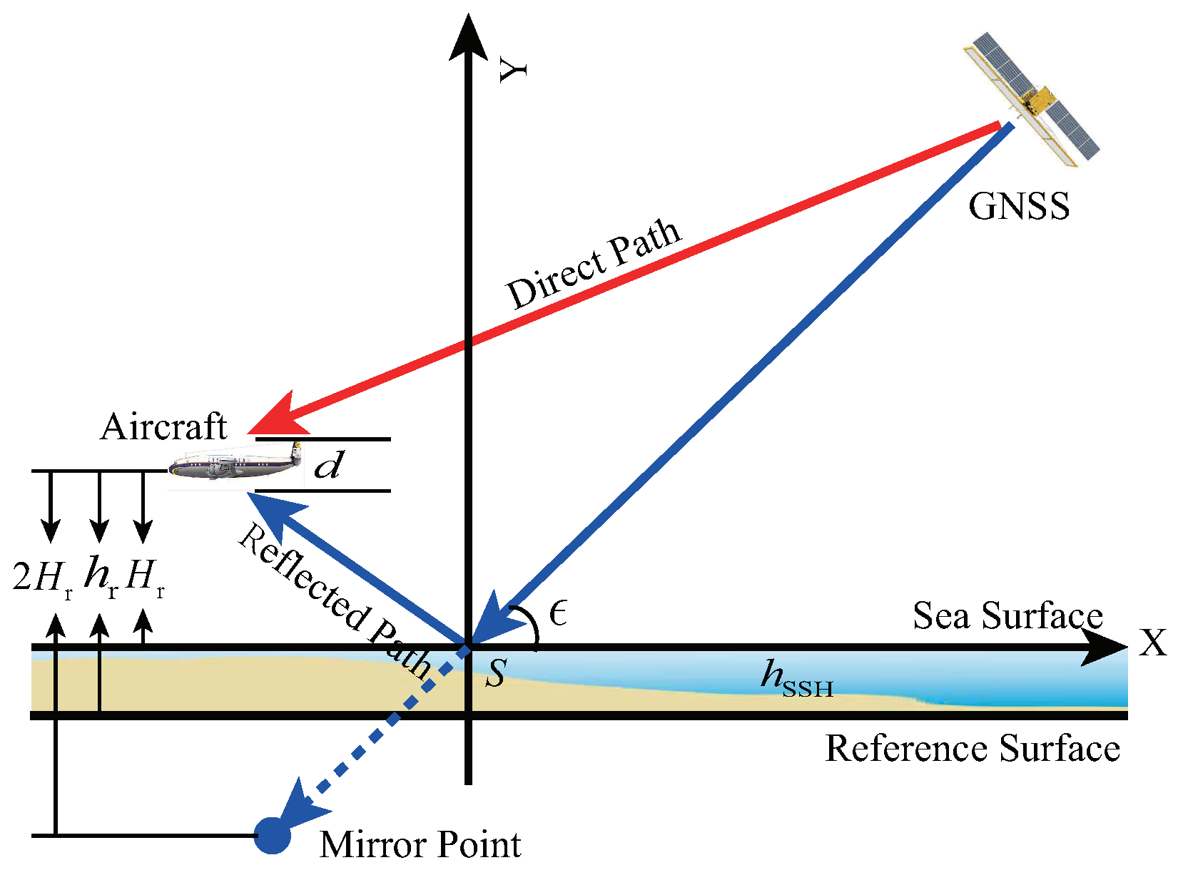
is the propagation delay of the direct and reflected signal, as shown in Figure 1, which is relative to the receiver height and the elevation angle of the GNSS satellite as
where is the elevation angle of the GNSS satellite and is accurately computed from the direct signal or IGS ephemeris, is the receiver height referring to the sea surface, and d is the distance between the up- and down-looking antennas. Once is computed from Equation (3), the sea surface height can be computed as
is the bias between the estimated delay by retracking the feature point and the specular delay and is called the specular delay bias. Precisely calibrating the above bias is important for improving the precision of the retrieved sea surface height.
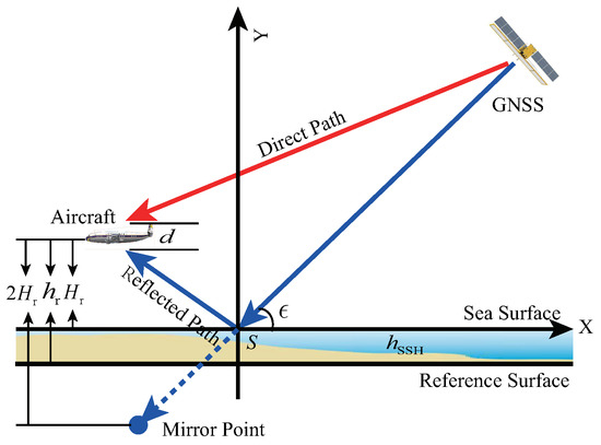
Figure 1.
Geometry of measuring the sea surface height using airborne GNSS reflectometry.
2.2. Delay Estimation
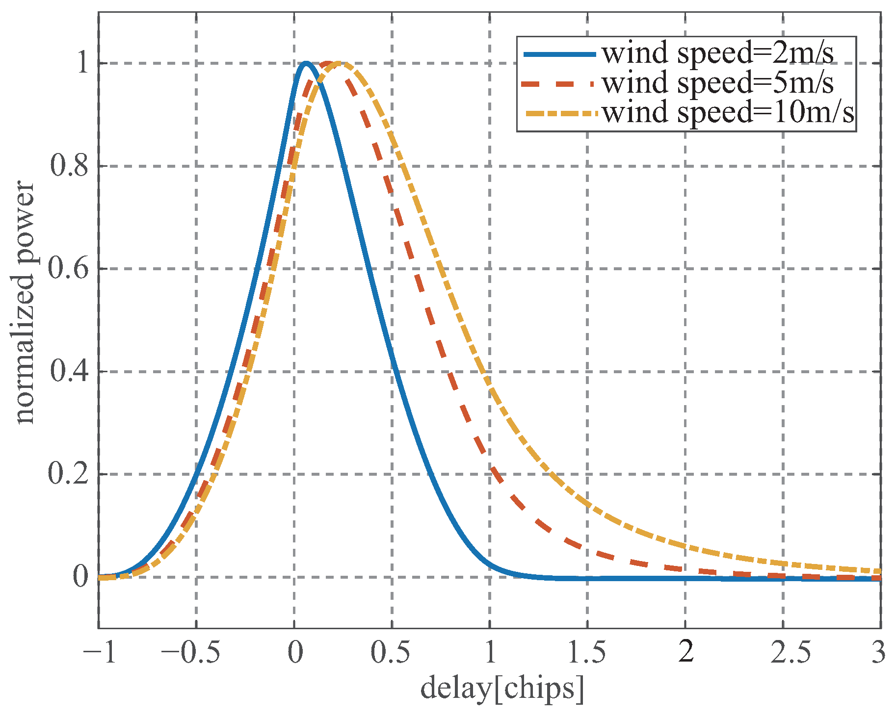
The receiver height referring to the sea surface can be obtained using the geometry of GNSS reflectometry and is important for estimating the delay between reflected and direct signals from the measured waveform. At present, two schemes, including retracking given points [27,28,29] and fitting models [30], have been utilized. The method of retracking a given point is used in this paper because of the low complexity of this technique. A retracked point in the reflected waveform that is easy to extract from the waveform and is rarely influenced by the noise and sea state should be defined. As presented in Figure 2, which shows the simulated delay waveforms used the Z-V model [31] for different wind speed, compared to the waveform peak and trailing edge of the waveform, the leading edge is relatively insensitive to the sea state. The peak of the derivative waveform is chosen as the retracked point to estimate the arrival time of the reflected signal and corresponding delay is defined as
where is the delay waveform of the reflected signal. The peak of the derivative waveform is used in this paper to estimate the delay of reflected signals. The sparse sampling waveform is first interpolated to produce the dense-sampling waveform, and then the interpolated waveform is differentiated and searched for the peak of the derivative waveform. The alternative approach is to first use a polynomial to fit the leading edge of the measured waveform and then analytically compute the zero-crossing point of the second derivative of the fitted polynomial [33]. In this paper, the first method is used to retrack the peak delay of the derivative waveform.
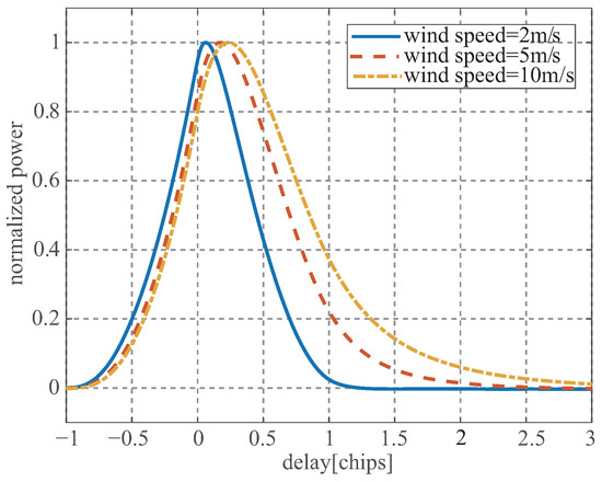
Figure 2.
Simulated reflected waveforms for wind speeds of 2, 5, and 10 m/s.
3. Specular Delay Bias
For an idealized situation in which the impulse response starts to spread from the specular delay to a longer delay, the specular delay is theoretically the same as the delay of the peak of the derivative waveform [27]; however, the actual scenario is complete, so the specular delay has a bias from the delay estimated using the peak of the derivative waveform; this bias should be evaluated and calibrated. In [29], the delay derived using the peak of the derivative waveform is calibrated with a correlation computed from the modeled waveform. To further analyze the specular delay bias, the waveform model of reflected GNSS signals is used [31].
where and are the transmitted signal power and transmitting antenna gain, respectively; is the antenna gain of the receiver; is the wavelength of the GNSS signal; and are the distances from the receiver and the GNSS satellite to the observation area, respectively; is the autocorrelation function of the pseudorandom noise (PRN) code; and is the scattering coefficient from p polarization to q polarization, which could be computed using Equation (34) in [31].
3.1. Elevation Angle
The reflected GNSS signals depend on the surface roughness. The criterion usually used to distinguish smooth and rough surfaces is the Rayleigh criterion, as in [34]
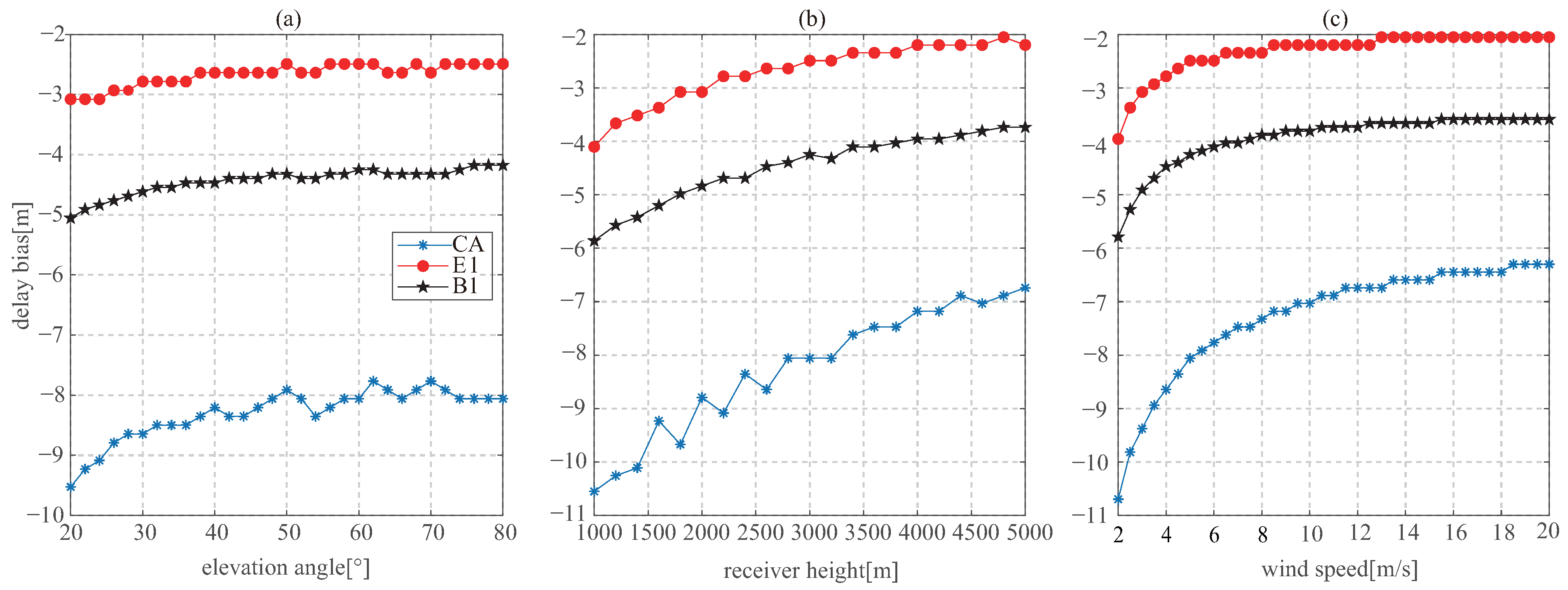
For a satellite with a lower elevation angle under the same sea state conditions, the surface is smoother, so the delay waveform is more similar to that of the direct signal and the arrival time of the specular signal is closer to the peak of the delay waveform. Figure 3a shows the changing delay bias versus the elevation angle for GPS CA, Galileo E1b, and BeiDou B1I when the height and wind speed are 3500 m and 5 m/s, respectively, in which the peak delay of the derivative waveform has a negative bias relative to the specular delay and increasing the elevation angle makes the bias lower and ultimately converge to a stable value.
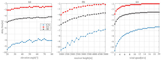
Figure 3.
Variation in the bias with increasing (a) elevation angle for the case of the height of 3500 m and wind speed of 5 m/s; (b) height for the case of the elevation angle of and the wind speed of 5 m/s and (c) wind speed for the case of the elevation angle of and the height of 3500 m.
3.2. Height
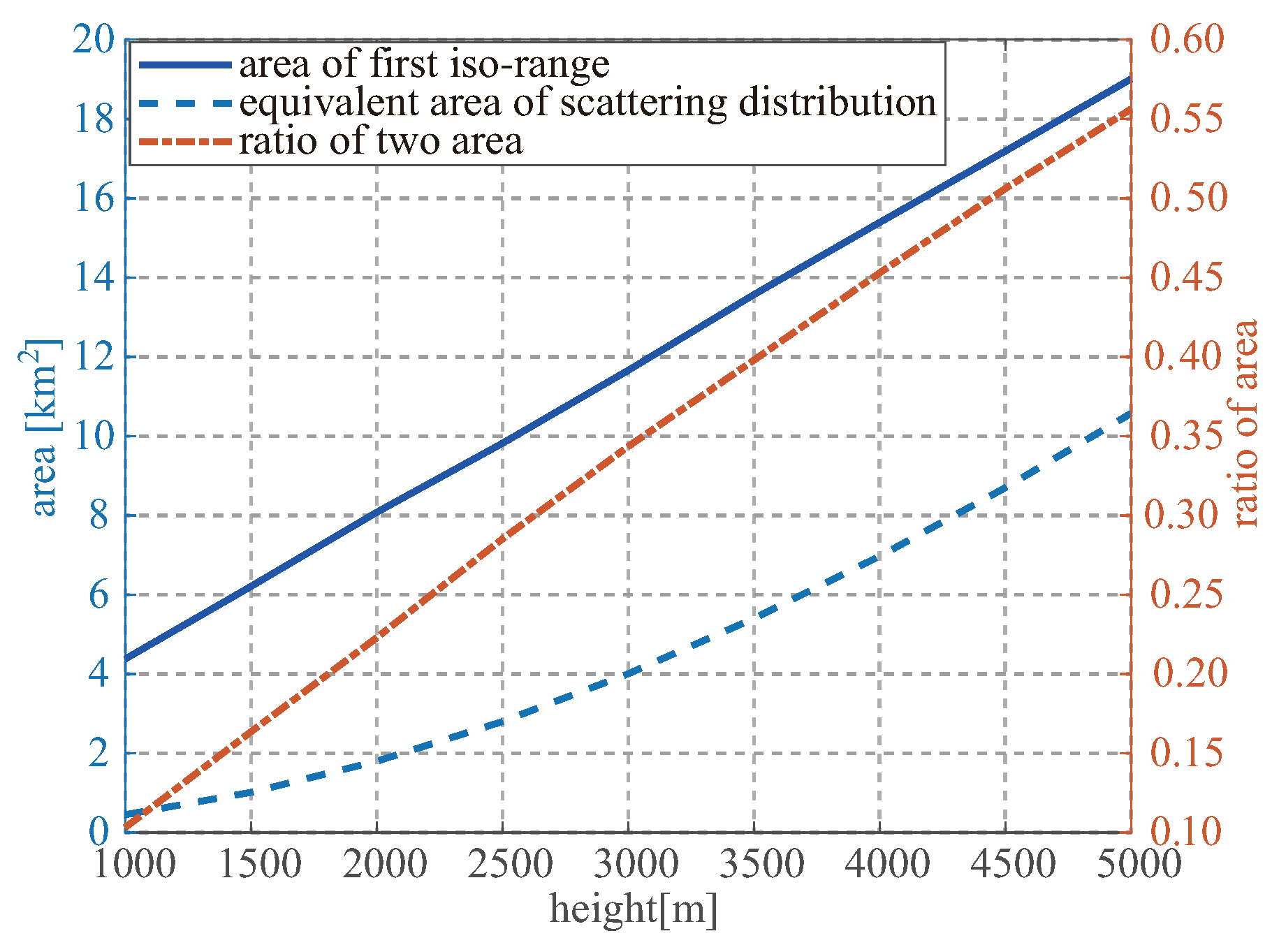
For the diffuse reflection, the reflection zone is jointly determined by the first isorange and glistening zone. The size of the first isorange is computed by , where a and b are the semimajor and semiminor axes of the first isorange, which are estimated through Equation (3) in [35]. The size of the glistening zone is defined as the equivalent area of the scattering coefficient by
where is the peak of the scattering coefficient and computed as (where is the maximum operator); represents the scattering area. As shown in Figure 4, as the receiver height rises, the area of the first iso-range shows the approximately linear growth; however, the equivalent area of the scattering distribution presents the exponential growth. Therefore, the ratio between the equivalent area of the scattering distribution and the area of the first isorange shows an increasing trend. For a lower receiver height, the glistening zone is smaller than the ellipse of the first iso-range and the delay waveform is similar to the ideal triangle function. In this case, the optimal feature point to estimate the specular delay is the waveform peak rather than the peak of the derivative waveform. This illustrates the phenomenon shown in Figure 3b which shows that the lower the receiver height is, the larger the specular delay bias is.
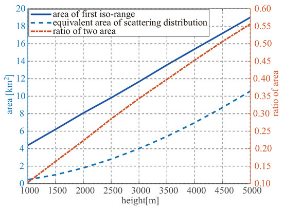
Figure 4.
Area of the first isorange, equivalent area of the scattering distribution, and their ratio versus the receiver height for an elevation angle of and a wind speed of 5 m/s.
3.3. Wind Speed
Figure 3c gives the specular delay bias with respect to the wind speed. The absolute bias presents a decreasing trend as the wind speed increases and becomes stable after 12 m/s. For the case of a lower wind speed, the scattered signals come from the zone with the shorter delay, and the delay waveform is more similar to the triangle function than the peak of the derivative waveform; therefore, the delay estimated by the peak of the derivative waveform has more severe bias. Note that for the relatively calm sea surface, specular reflection occurs and coherency properties of specular scattering can be observed [36], and the coherent components coming from the Fresnel zone dominate the reflected signals. In this case, the delay waveform is identical to that of the direct signal, so the unbiased estimation of specular delay can be obtained by retracking the waveform peak.
3.4. Pseudorandom Noise Code
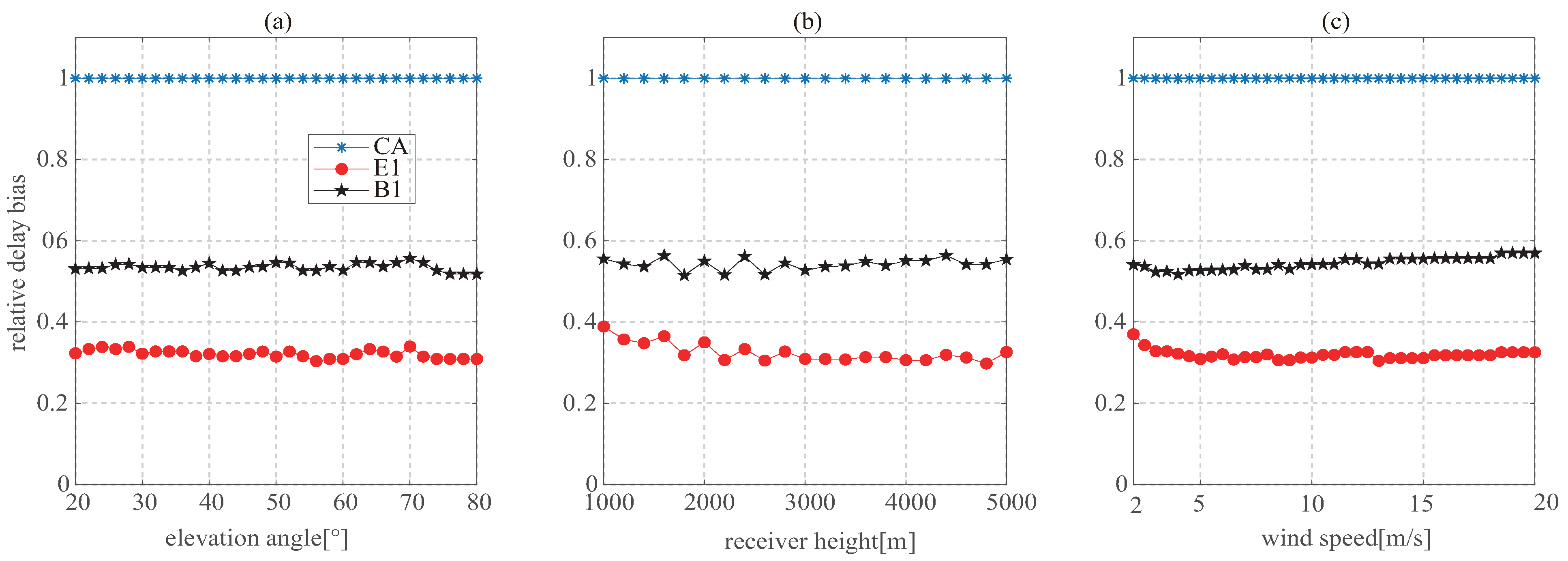
The PRN code has an important influence on the estimated delay. A code with a wider bandwidth produces sharper edges, which enables more accurate and precise estimation. The Cramer-Rao bound (CRB) of the ranging precision is inversely proportional to the square of the signal bandwidth [37]. Equation (6) can be written as the convolution between and the bistatic radar cross-section including the relative position between the transmitter and the receiver, the sea surface parameters, and the antenna footprint. Intuitively, the impact of the PRN code on delay bias is uncoupled from the elevation angle, receiver height, and wind speed. The Z-V model is used to simulate and demonstrate this intuition. Figure 5 shows the simulated biases which are normalized by the bias of GPS CA versus the elevation angle, receiver height, and wind speed. The normalized bias of Galileo E1b presents weak fluctuations for the case of receiver heights lower than 1500 m or wind speeds less than 3 m/s. However, under the other conditions, the biases of Galileo E1b and BeiDou B1I are stable with respect to that of GPS CA. This illustrates that the bias of Galileo E1b and BeiDou B1I can be derived from that of GPS CA by multiplying by the constants 0.32 and 0.54 for Galileo E1b and BeiDou B1I, respectively. The above constants are computed through averaging the normalized biases of the Galileo E1 and BeiDou B1I in Figure 5.

Figure 5.
Normalized sea state bias of (a) GPS CA; (b) Galileo E1b and (c) BeiDou B1 relative to the bias of GPS CA for the same condition.
3.5. LHCP Antenna
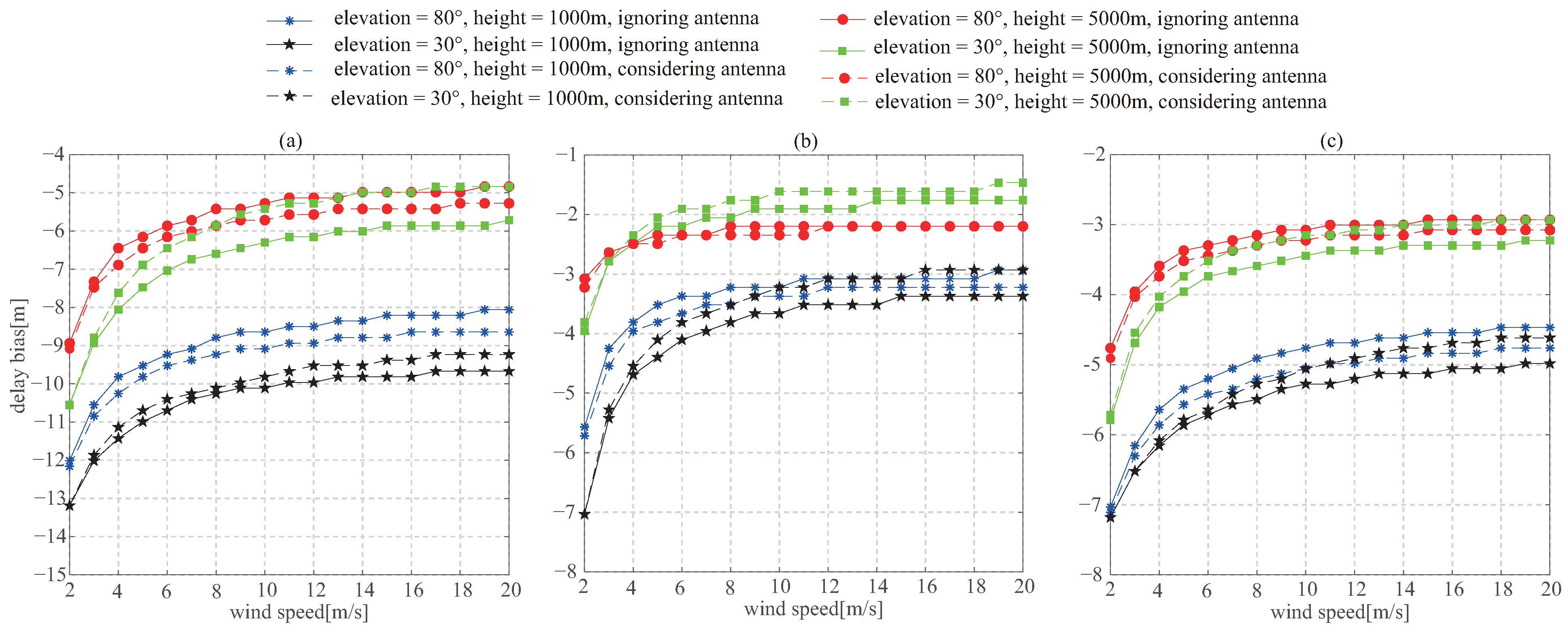
As shown in Equation (6), the antenna gain pattern modulates the signal from different directions. This modulation generates different deformations in the delay waveform from the different satellites. In this paper, only the case of the down-looking and circular-beam antenna with a gain of 12 dB and a beam width of is analyzed. Figure 6 gives the delay bias considering and ignoring the impact of the antenna gain pattern. The antenna pattern has a more serious influence on the delay bias in the case of high wind speed and low elevation angle. The bias difference between the considered and ignored impact of the antenna gain pattern is under 1 m. Due to the impact of the antenna gain pattern being lower than that of the elevation angel, receiver height, wind speed and PRN code, in the development of the calibration model of the delay bias in this paper, the antenna influence is ignored.
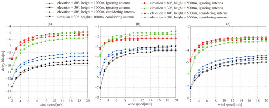
Figure 6.
Sea state bias ignoring and considering antenna modulation for (a) GPS CA; (b) Galileo E1b and (c) BeiDou B1.
4. Calibration of the Specular Delay Bias
When the influence of the antenna is ignored, the specular delay bias is jointly determined by the elevation angle, receiver height, wind speed, and PRN code by
where is the sine of the elevation angle, is the wind speed, is the parameter characterizing the impact of the PRN code, and represents the mapping relationship between the delay bias and its influencing factors.
4.1. Analytical Model
To develop the analytical calibration model, it is assumed that the influences of the elevation angle, receiver height, wind speed, and PRN code on delay bias are independent. It is known that the delay biases of Galileo E1b and BeiDou B1I are stable with respect to that of GPS CA and can be obtained from the delay bias of GPS CA through multiplication with constants. The analytical model is expressed as
of GPS CA, Galileo E1b, and BeiDou B1I are 1, 0.32 and 0.54, respectively. For the given reference of elevation angle, receiver height, and wind speed, the delay bias of GPS CA is
where is 1; , and are the sines of the referenced elevation angle, receiver height, and wind speed, respectively, which are , 1000 m, and 2 m/s in this paper. The delay bias of the reference case is derived through simulation using the theoretical model given by Equation (6). Here, , and are respectively defined as
Further work is needed to obtain the expressions of , and . For the referencing elevation angle, the delay bias is
Similarly, for the given receiver height and wind speed, the delay biases are
Similarly, and are respectively expressed as
The Monte Carlo method is used to obtain , and through the following steps:
- a group of elevation angles, receiver heights, and wind speeds are randomly generated and recorded as , respectively, where ;
- the elevation angle, receiver height, and wind speed in the above group are replaced with the given references to produce the other three groups, recorded as , and , respectively;
- the above four groups of parameters are used as the input to simulate the delay waveforms of GPS CA, Galileo E1b, and BeiDou B1I through Equation (6);
- the delay bias is estimated and recorded as , , and for GPS CA; , , and for Galileo E1b; and , , and for BeiDou B1I;
- , and are computed for GPS CA, Galileo E1b, and BeiDou B1I as
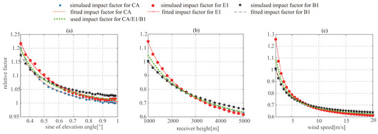
Figure 7.
Variation in the impact factor with increasing (a) elevation angle; (b) height, and (c) wind speed.
In addition, , and of GPS CA, Galileo E1b, and BeiDou B1I have similar changing tendencies and can share the same fitted parameters in Equation (25). The fitted parameters used in this paper are given in Table 1.

Table 1.
Fitted Parameters of the elevation angle, receiver height, and wind speed.
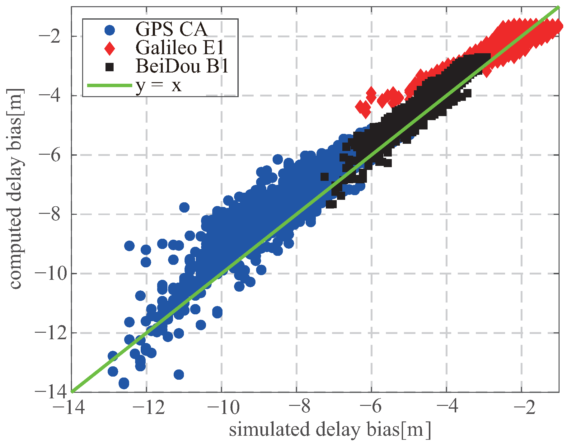
Figure 8 shows the simulated delay biases and delay biases computed using the above analytical calibration model, in which simulated and computed delay biases are consistent, and their root mean square errors (RMSEs) are 0.43, 0.29, and 0.18 m for GPS CA, Galileo E1b, and BeiDou B1I, respectively.
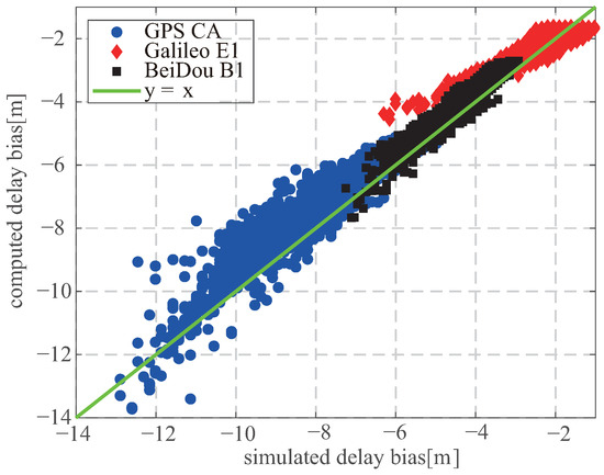
Figure 8.
Comparison of the simulated sea state bias and sea state bias computed using the analytical model (18).
4.2. Neural Network
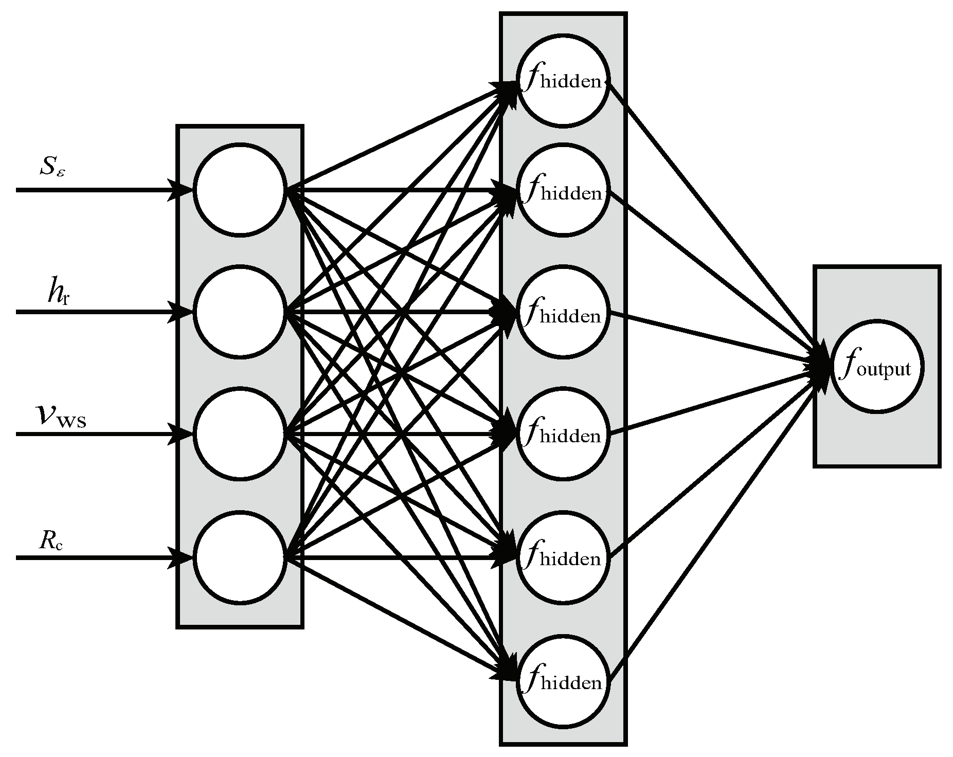
Artificial intelligence (AI) methods, such as neural networks [38], can be used to develop predictive models based on empirical data. In this paper, a back propagation (BP) network, as shown in Figure 9, is trained to develop the calibration model of the delay bias. The inputs of neural network are the sine of the elevation angle , height , wind speed , and . The output is the predicted delay biases. Note that of the neural network is quantified as 0, 1, and 2 for GPS CA, Galileo E1b, and BeiDou B1I signal. The data generated in Section 4 are randomly divided into two sets. One set which accounts for 70% of the total data used to train the neural network and the other set accounting for 30% of the total data is used to test the developed neural network. The ability to approximate the analytical function is dependent on the number of hidden neurons and activation functions [39]. The usually used activation functions are purelin, tanh, and sigmoid function. Table 2 gives the RMSEs of the biases in test set for the different combinations of the activation function in hidden and output layer when the hidden node number is 6. From the table, it is seen that when the activation functions in hidden and output layer respectively are tanh and purelin function, the RMSEs are relatively low. Therefore, in this paper the following tanh and purelin functions are used as the activation functions in the hidden and output layers of the neural network.
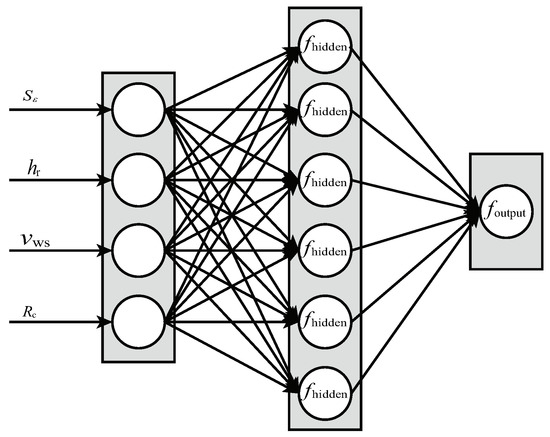
Figure 9.
Structure of the adopted neural network.
Table 2.
Parameters of the simulation scenario.
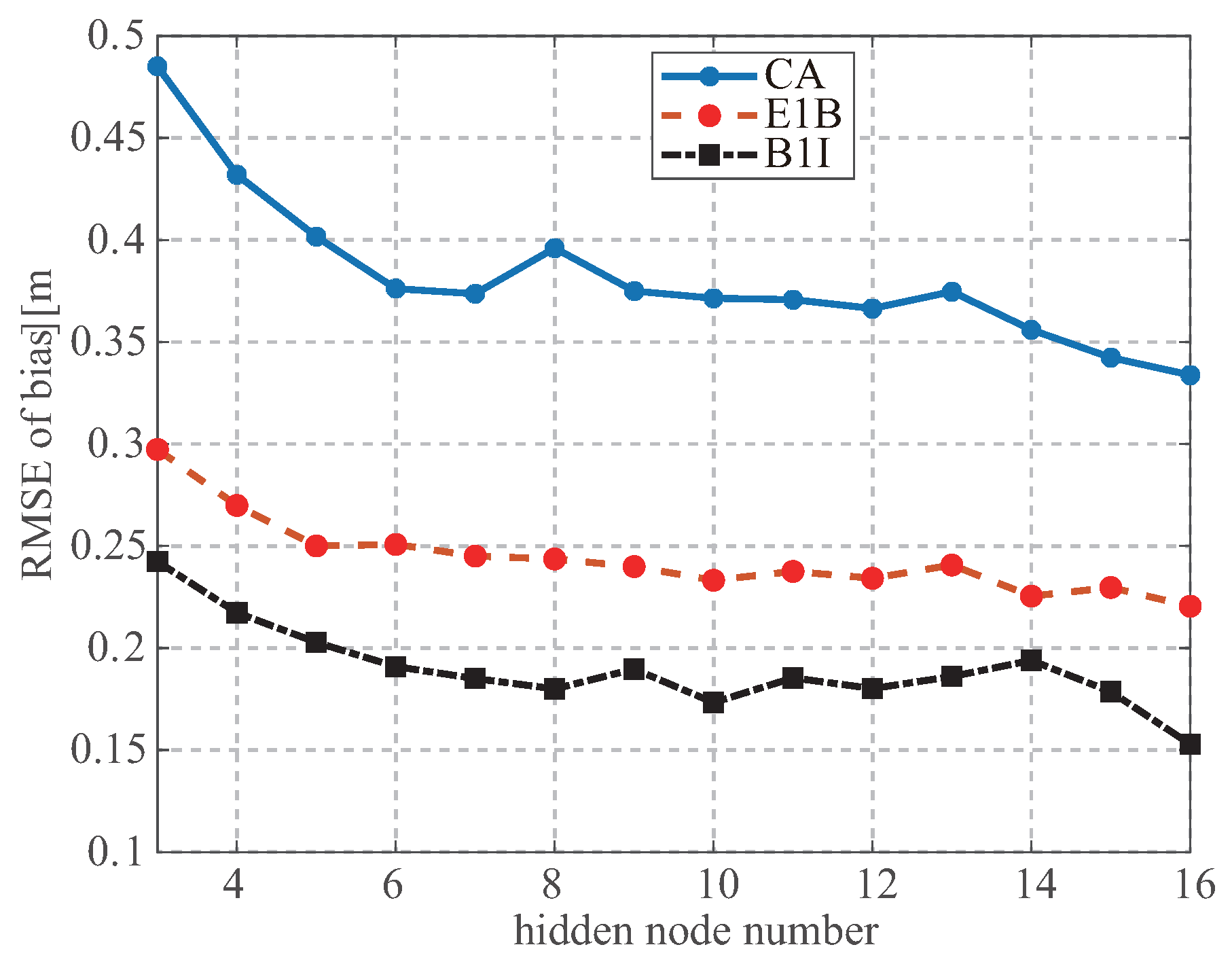
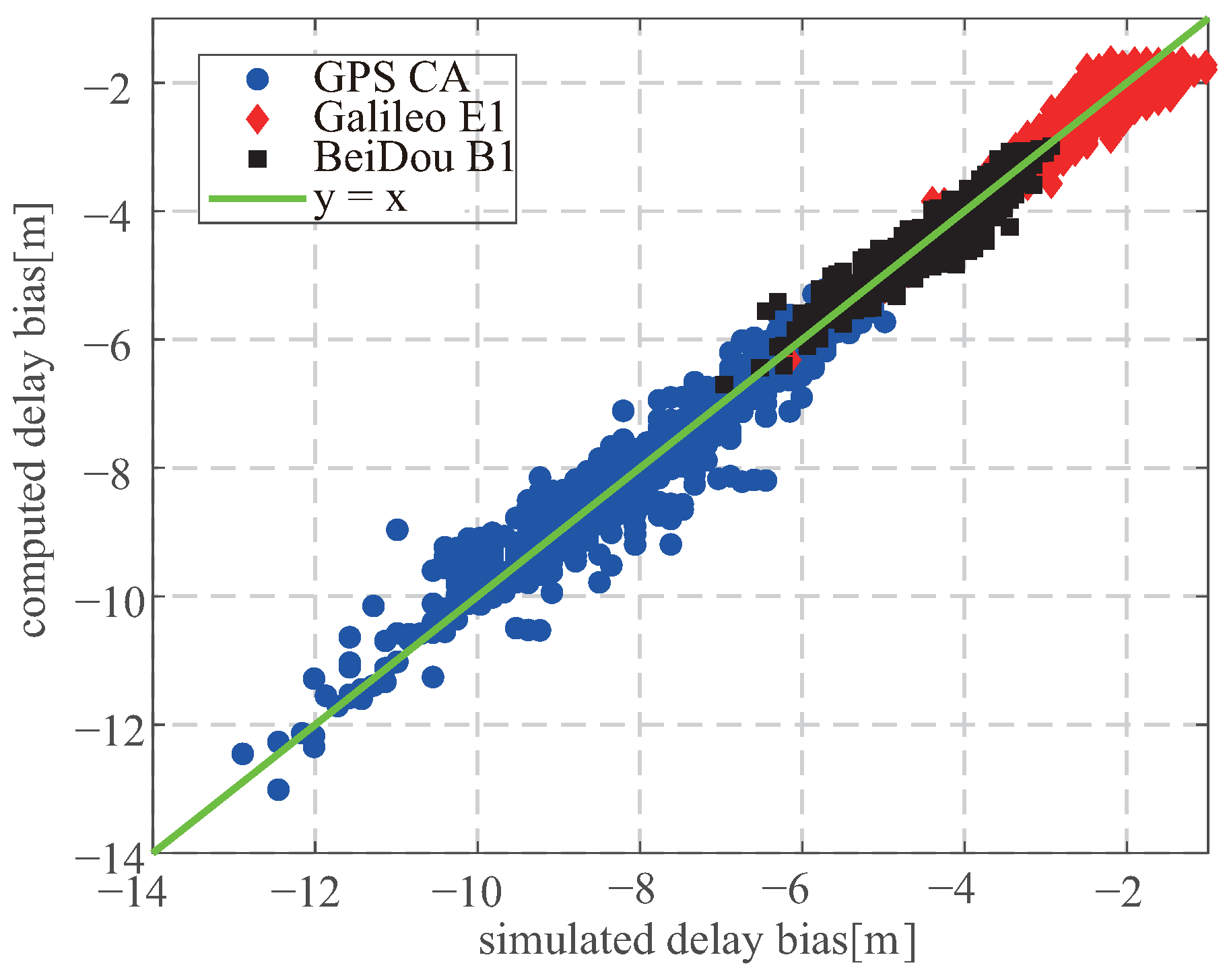
From Figure 10, it is clear that the RMSEs of the biases in test set for GPS CA, Galileo E1b, and BeiDou B1I are all decreasing as the hidden node number increases and becomes stable after the hidden node number is 6. Therefore, the neuron number of the hidden layer in this paper is 6. Figure 11 gives the simulated delay biases and delay biases computed using the developed neural network model, in which the RMSEs of GPS CA, Galileo E1b, and BeiDou B1 are 0.38, 0.26, and 0.16, respectively, which are slightly better than those of the above analytical model.
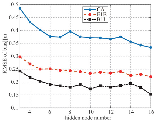
Figure 10.
RMSEs of GPS CA, Galileo E1b, and BeiDou B1I for the different node number in hidden layer.
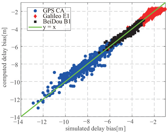
Figure 11.
Comparison of the simulated sea state bias and sea state bias computed using neural network.
4.3. Multisatellite Observation
The analytical model and neural network above require information about the elevation angle, receiver height, and wind speed. The elevation angle and receiver height can be obtained from the direct signal. In addition to the existing methods for obtaining wind speed such as scatterometers and nearshore buoys, reflected GNSS signals provide wind speed by best matching the measured delay waveform to the theoretical delay waveform for airborne scenarios [40]. Whether the delay bias can be calibrated for the case of unknown wind speed should be explored. It is known that the specular points of several satellites are visible for a down-looking antenna. Assuming that the wind speed is identical in the coverage of the down-looking antenna, in Equation (16) is the same for different satellites. The Equation (16) is expressed as
where . When the down-looking antenna covers N specular points, calibration models of N satellites can be expressed as
where , and are respectively expressed as
in Equation (29) could be solved through least square as
Assuming that the measurements of different satellites are independent and that the errors are subject to the normal distribution, the mean and variance of the measurement error are and , respectively. The covariance matrix of is . The covariance matrix of is derived as
where is the error vector of the measurement . From the above equation, it is seen that the height variance measured using multi-observation is not only dependent on the variance of the estimated delay but also influenced by a weight coefficient as
where . From the above equation, it is seen that the variance of the height is dependent on the elevation angle and PRN code. When the delay waveforms used for the multi-observation have the same PRN type and elevation angle, the variance of the height tends to infinity; in other words, is under rank, and Equation (32) is an underdetermined equation that has innumerable solutions. To obtain the proper height, two conditions are required:
- The elevation angles of the chosen satellites should be as different as possible;
- The frequency spectra of the delay waveform should be as different as possible.
5. Validation
Simulations and experiments are performed to demonstrate the validity of the proposed calibration models.
5.1. Simulation
The complex correlation value of the reflected signal in the presence of noise can be modeled as [41]
where and are complex Gaussian white noise with real and imaginary parts; is the noise power, which is expressed as [42]
where is the coherent integration time, k is the Boltzmann constant, is the receiver noise equivalent temperature, and is the receiver bandwidth. To obtain waveforms with different SNRs, the noise power is multiplied by a factor as . The above complex correlation waveforms are incoherently averaged as
where N is the incoherent averaging number.
The simulation scenario is shown in Figure 12 and Table 3, in which the chosen flight area is located in the South Sea in China. The flight height is 3500 m, and the sea surface height is 0.16 m. The wind speed from global numerical ocean models changes from 3.85 to 4.15 m/s. The satellite position and velocity of GPS, Galileo, and BeiDou are computed through the official ephemeris. The satellites with PRNs of 6, 17, and 18 for GPS, 6 and 7 for Galileo and 1, 3, 10, 18, and 24 for BeiDou are visible to both up-looking and down-looking antennas.
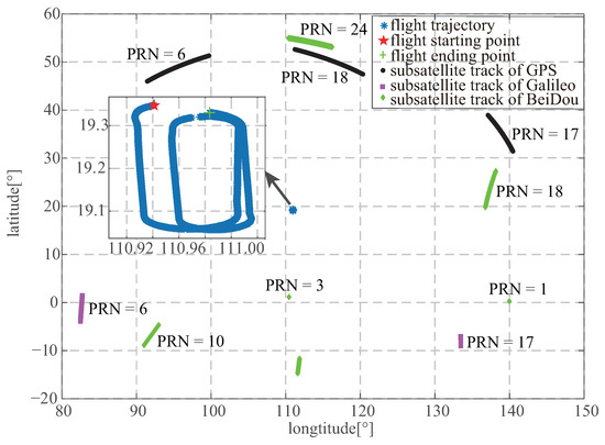
Figure 12.
Flight trajectory and subsatellites of GPS, Galileo, and BeiDou for the simulation scenario.
Table 3.
Parameters of the simulation scenario.
Here, the GPS PRN 18 satellite, with elevation angle ranging from to ; Galileo PRN 6 satellite, with elevation angle ranging from to ; and BeiDou PRN 10 satellite, with elevation angle ranging from to ; are selected to validate the proposed calibration models. Table 4 and Table 5 give the bias and RMSE of the retrieved height before and after the calibration. The calibration is unable to improve the RMSEs of the retrieved sea surface height, and the RMSEs after calibration and without calibration are both at the decimeter level. In addition, Galileo E1b and BeiDou B1I yield lower RMSEs than GPS CA because of the wider frequency spectrum. The results of Table 4 show that the uncalibrated biases are −5.41, −1.68, and −2.77 m, and after calibration using the proposed models, the biases decrease to the decimeter level. This illustrates that the proposed models can significantly calibrate the delay bias.
Table 4.
Biases of the Retrieved Sea Surface Height Compared to the Height of DTU10 for the Simulated Scenario.
Table 5.
Root Mean Square Error of the Retrieved Sea Surface Height Compared to Height of DTU10 for the Simulated Scenario.
To illustrate the influence of matrix on the RMSE of the retrieved height, GPS PRN 07, 17, and 18 given in Table 6 are chosen to retrieve the sea surface height using multi-observations. The elevation angles of the three satellites are close, and the values are all 1; therefore, the matrix is perishing in the solution of Equation (33). In this case, the bias and RMSE of the retrieved height are −0.63 and 11.10 m, respectively, which are worse than the RMSE before the calibration. The corresponding is 102.74, which is much larger than the 0.96 of the combination of GPS PRN 18, Galileo PRN 06, and BeiDou PRN 10. Comparing the results of two multisatellite observations demonstrates that the geometric configuration is important for achieving proper calibration and preventing the RMSE of the retrieved height from increasing. A suitable configuration should have as different of elevation angles and frequency-spectrum waveforms as possible.
Table 6.
Elevation Angle of GPS satellite Used to Illustrate the Influence of Matrix on the RMSE of Retrieved height.
5.2. Experiment
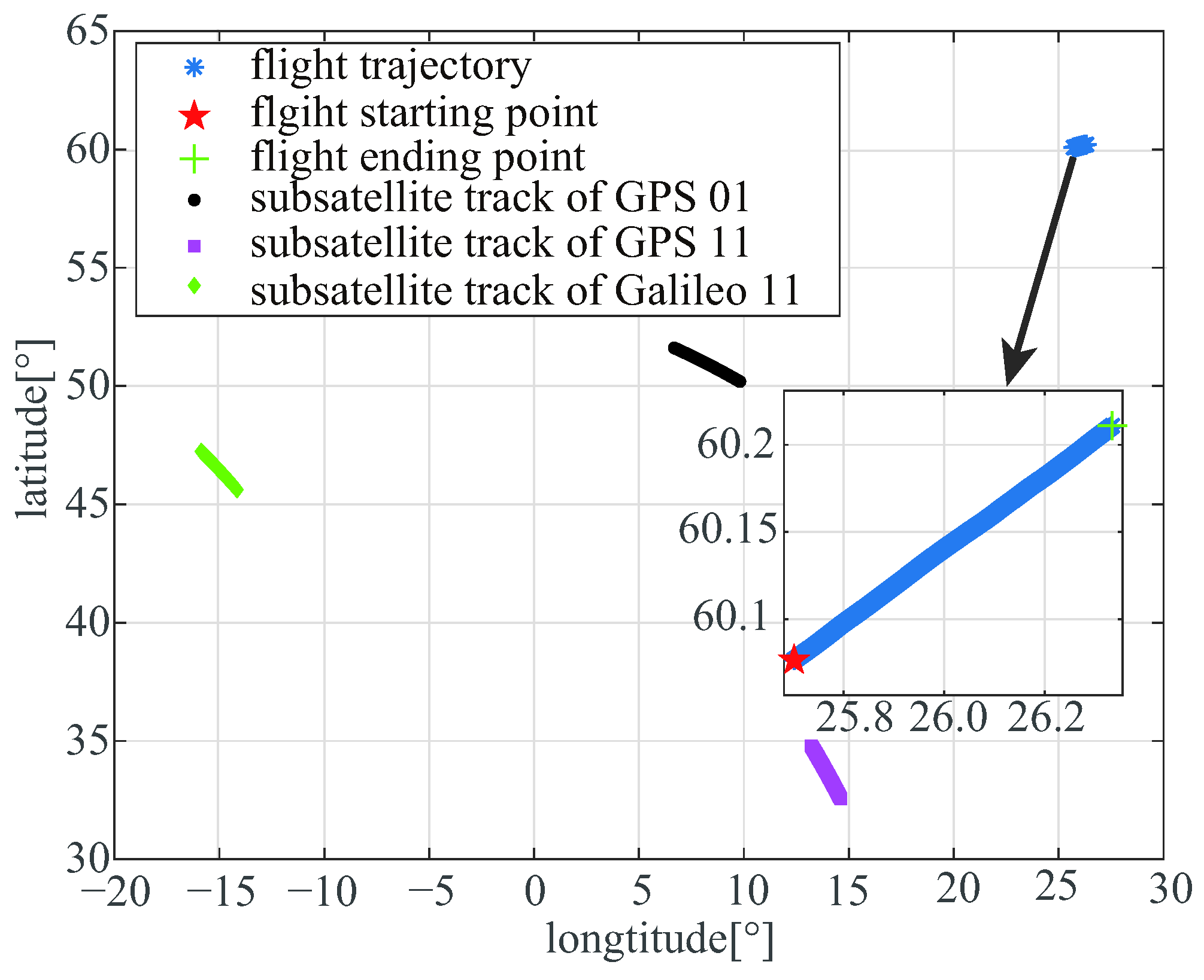
The dataset used in this paper was collected during an airborne experiment over the Baltic Sea on 3 December 2015. Two 8-element antennas were installed at the aircraft. One is the up-looking antenna, and the others is the down-looking antenna. RF chains with a sampling rate of 80 MHz, IF of 19.42 MHz, and quantization of 1 bit were used to collect the direct and reflected GNSS signals. The L1 signal of the GPS and E1b signal of Galileo were collected between seconds of the day (SoD) 39,217 and 39,617. During this period, the aircraft flew at an altitude of ∼3 km and a velocity of ∼50 m/s. As shown in Figure 13, PRN01 and 11 of GPS and PRN11 of the Galileo System were visible for both the up-looking and down-looking antennas. The elevation angles of these three satellites are computed using IGS ephemeris and present ranges of ∼, ∼ and ∼, respectively. The amplitude of the tides is just a few centimetres in the Baltic Sea, and the salinity, temperature, precipitation, and evaporation also have minor effect on the Baltic sea level [43]; the sea surface height from the DTU10 model [44] is considered the ground truth for comparison with the retrieved sea surface height using the reflected GPS and Galileo signals.
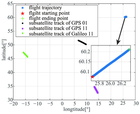
Figure 13.
Flight trajectories and subsatellites of GPS and Galileo for the experimental campaign.
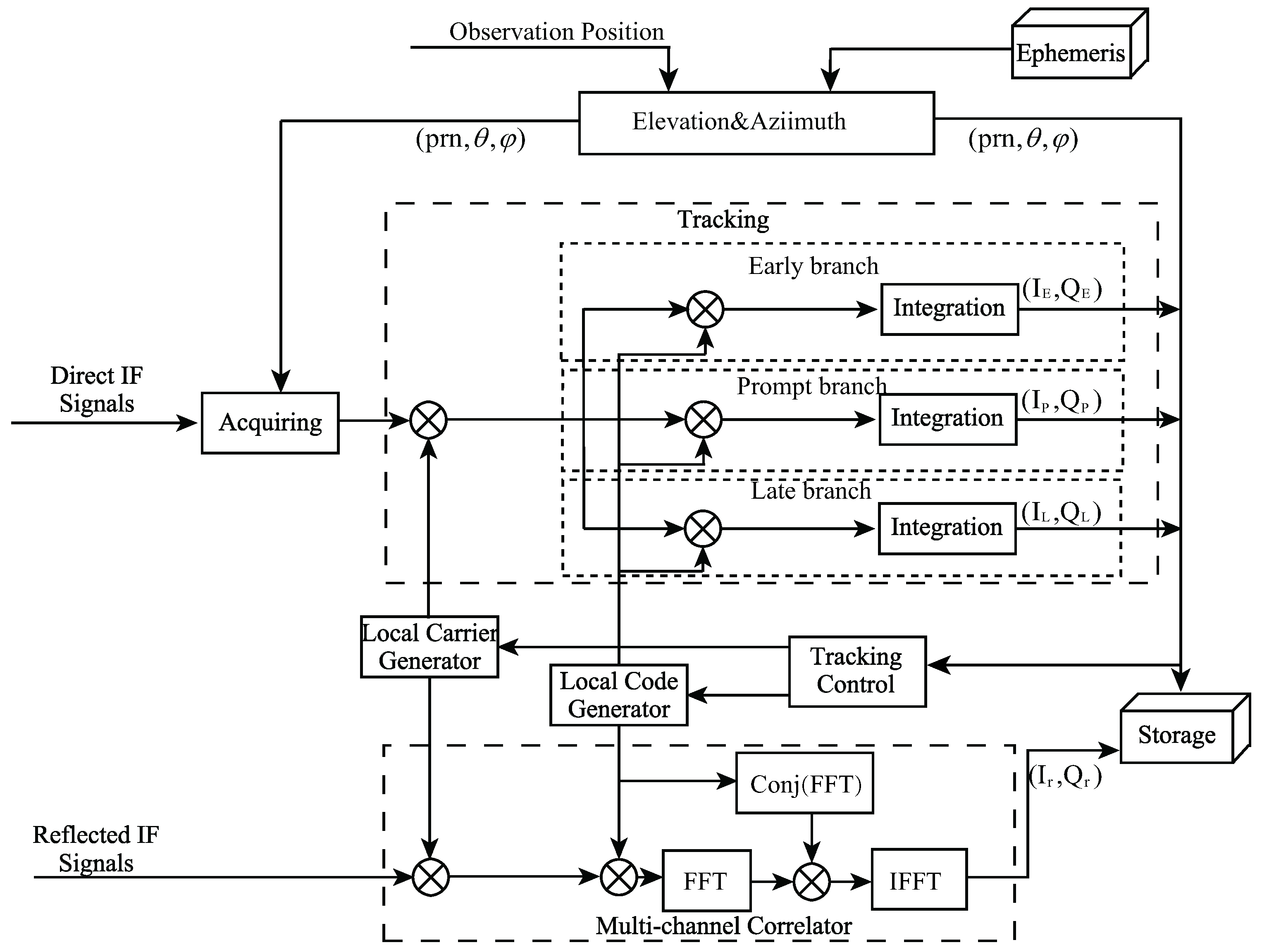
A software receiver, as given in Figure 14, is developed to obtain the delay waveform of the reflected GPS and Galileo signals. The software receiver consists of direct and reflected channels for processing direct and reflected GPS and Galileo signals. The direct and reflected channel share the local replicas from the local signal generator in Figure 14. The direct signals are acquired and tracked to provide a reference for the processing of the reflected signals. The code parallel algorithm in frequency domain is used to accelerate the acquiration procedure of the direct signal. The Phase Locked Loop (PLL) and Delay Locked Loop (DLL) are respectively adopted to dynamically track the carrier and code phase of the direct signal. The detail processing of the direct signal could be seen in [45]. The reflected channel is composed of a set of correlators that perform cross-correlation between the reflected signals and the local replica at different delays. To improve the processing efficiency of the reflected signals, cross-correlation in the frequency domain using the fast Fourier transform (FFT) is implemented. The coherent integration time in the software receiver is the same as the period of the PRN code, i.e., 1 ms and 4 ms for the GPS and Galileo signals, respectively. After cross-correlation, a series of complex correlation waveforms are incoherently averaged to improve the SNR of the waveform. To ensure an output rate of 1 Hz, the incoherent averaging numbers for the waveforms of GPS and Galileo are 1000 and 250, respectively. The ephemeris is used to compute the elevation angles of the satellites.
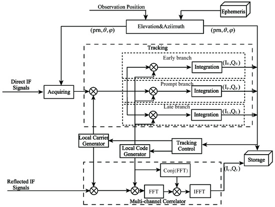
Figure 14.
Processing structure of the direct and reflected GNSS signals.
The following steps are conducted to retrieve the sea surface height:
- The receiver position and elevation angle of the GNSS satellite are computed from the direct signal and IGS ephemeris;
- The peak of the derivative waveform is retracked to estimate the delay from the incoherently averaged waveforms;
- and are calibrated to obtain ;
- Equation (3) is used to compute the receiver height referring to the sea surface;
- The sea surface height is retrieved using Equation (4), and a moving average is obtained for the retrieved heights;
- A comparison is made with the DTU10 data to obtain the bias and RMSE of the retrieved sea surface height.
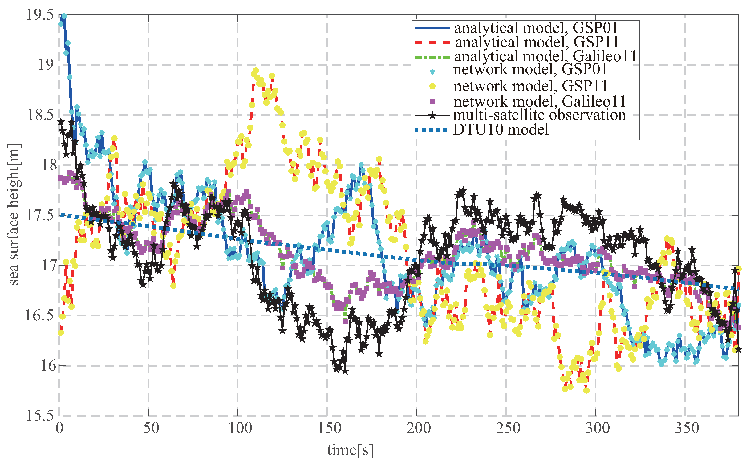
Figure 15 shows the in situ and retrieved sea surface heights, and both present the same trend. Table 7 and Table 8 give the bias and RMSE of the retrieved height, respectively. Similar to the results of the simulation, decimeter-level RMSE can be obtained both before and after the calibration, and the RMSE of Galileo E1b is lower than that of GPS CA. In addition, PRN 01 of GPS yields a better RMSE than PRN 11. This occurs because the larger the sine of the elevation angle is, the higher the retrieved precision is [46]. Meter-level bias is present before the calibration, and decimeter-level bias is achieved after the calibration.
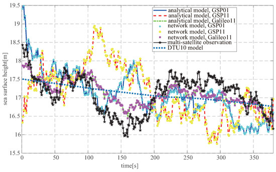
Figure 15.
Retrieved and in situ sea surface height.
Table 7.
Biases of the Retrieved Sea Surface Height Compared to the Height of DTU10 for the experimental campaign.
Table 8.
Root Mean Square Error of the Retrieved Sea Surface Height Compared to the Height of DTU10 for the experimental campaign.
To validate the influence of the selection of satellites on the height using multisatellite observations, the heights of different configurations are obtained. Table 9 shows that the GPS PRNs of 01 and 11 yield different elevation angles; however, enlarges, so the bias and RMSE of the retrieved height are unacceptable. When GPS PRN 11 and Galileo PRN 11, which have similar elevation angles, are chosen, proper results are achieved. This is mainly because, as shown in Figure 3, when the elevation angle is over , the elevation angle has an insignificant effect.
Table 9.
Root Mean Square Error of the Retrieved Sea Surface Height Compared to the Height of DTU10 for the experimental campaign.
6. Discussion
This paper proposes three methods for calibrating the delay bias; however, after the calibration, the bias of the retrieved height is still at the decimeter level. Theoretically, fitting a model to the measured waveform may produce unbiased estimation; however, note that the matching procedure is computationally complex and that its retrieved performance depends on the theoretical model used. Therefore, to fit a model, it is important to develop a precise waveform model. The model currently usually used (the Z-V model) was proposed by V. U. Zavorotny et al. [31] based on the Kirchhoff approximation and geometrical optics (KA-GO); this model describes the power distribution of the scattered GNSS signal and has been used to approximate the measured waveform. However, the Z-V model ignores the coherent component in the reflected signal. For some cases, such as calm seas and lakes, strong coherent scattering in the near-forward bistatic geometry takes place. In these scenarios, the Z-V model produces an incorrect result for the fitting of the measured waveform.
The comparison between the retrieved results of the GPS L1 CA and Galileo E1b code clearly shows that the E1b code yields better performance than the CA code because of the wider signal bandwidth. iGNSS-R was proposed because it can use the full-bandwidth signal to obtain higher precision in altimetry. At present, to use wide-bandwidth signals, especially encrypted signals, such as the P(Y) code of GPS, some approaches have been proposed, including partial interferometer [47] and semicodeless technology [48]. In addition, due to the wider frequency spectrum, some other signals from communication satellites have been used to provide more precise altimetry [49]. The proposed methods can also be used to calibrate the bias of the above signals; however, the fitting parameters of the analytical models have to be obtained, and the neural network should be trained again.
7. Conclusions
This paper analyzed the bias of the delay estimated by retracking the peak of the derivative delay waveform. The results showed that the elevation angle, receiver height, wind speed, PRN code, and down-looking antenna pattern influenced the delay bias. The impact of the PRN code was uncoupled from the elevation angle, receiver height, and wind speed, so the delay biases of Galileo E1b and BeiDou B1I could be obtained from the bias of GPS CA by multiplication with the constants 0.32 and 0.54, respectively. From the assumptions that the effects of the elevation angle, receiver height, and wind speed on the delay bias were uncoupled and coupled, an analytical model and a neural network, respectively, were proposed to calibrate the delay bias. Simulations and experiments were conducted to validate the proposed models. The results showed that through calibration using the proposed models, the biases of the retrieved height were reduced to the decimeter level from the meter level. Because the reflected GNSS signals from several satellites could be received, multisatellite observations were used to calibrate the delay bias under the condition of unknown wind speed. The results of the simulation and experiment illustrated that the calibration performance depended on the chosen satellites, which had different elevations and PRN codes. However, in this paper, after calibration, the decimeter-level bias and RMSE of the retrieved height were achieved, and it is necessary to pursue a measured height with a lower bias and RMSE. Therefore, in the future, work exploring the measurement of the height using wider-spectrum signals, such as L5 of GPS and B3I of BeiDou, will be conducted to obtain better altimetry performance.
Author Contributions
Conceptualization, F.W. and B.Z.; methodology, F.W. and D.Y.; software, G.Z. and F.W.; validation, J.X., L.Y., and F.W.; investigation, L.Y.; writing—original draft preparation, F.W. and D.Y.; writing—review and editing, F.W. and D.Y.; visualization, F.W.; funding acquisition, F.W. and D.Y. All authors have read and agreed to the published version of the manuscript.
Funding
This research was funded by the China Postdoctoral Innovative Talent Support Program (BX20200039), the National Natural Science Foundation of China (41774028), and (31971781).
Institutional Review Board Statement
Not applicable.
Informed Consent Statement
Not applicable.
Data Availability Statement
The datesets of simulation analysis and validation are managed by the School of Electronics and Information Engineering, Beihang university; the datasets of the experiment are owned by the Institute of Space Sciences of Spain.
Acknowledgments
The authors would like to thank the Institute of Space Sciences in Spain for sharing the acquired GPS CA and Galileo E1b signal data for the validation in this paper and Professor Ernesto Lopez-Baeza at Valencia University for the improvements to the manuscript.
Conflicts of Interest
The authors declare no conflict of interes.
References
- Martin-Neira, M. A passive reflectometry and interferometry system (PARIS): Application to ocean altimetry. ESA J. Eur. Space Agency 1993, 17, 331–355. [Google Scholar]
- Yu, K.; Rizos, C.; Dempster, A. Sea surface altimetry based on airborne GNSS signal measurements. In Proceedings of the International Society for Photogrammetry, and Remote Sensing (ISPRS) Congress, Melbourne, Australia, 5 August–1 September 2012; pp. 347–352. [Google Scholar]
- Clarizia, M.P.; Ruf, C.; Cipollini, P.; Zuffada, C. First spaceborne observation of sea surface height using GPS-Reflectometry. Geophys. Res. Lett. 2016, 43, 767–774. [Google Scholar] [CrossRef] [Green Version]
- Li, Z.; Zuffada, C.; Lowe, S.T.; Lee, T.; Zlotnicki, V. Analysis of GNSS-R Altimetry for Mapping Ocean Mesoscale Sea Surface Heights Using High-Resolution Model Simulations. IEEE J. Sel. Top. Appl. Earth Obs. Remote Sens. 2016, 9, 4631–4642. [Google Scholar] [CrossRef]
- Clarizia, M.P.; Ruf, C.S. Wind speed retrieval algorithm for the cyclone global navigation satellite system (CYGNSS) mission. IEEE Trans. Geosci. Remote Sens. 2016, 54, 441–4432. [Google Scholar] [CrossRef]
- Foti, G.; Gommenginger, C.; Jales, P.; Unwin, M.; Shaw, A.; Robertson, C.; Rosello, J. Spaceborne GNSS reflectometry for ocean winds: First results from the UK TechDemoSat-1 mission. Geophis. Res. Lett. 2015, 43, 767–774. [Google Scholar] [CrossRef] [Green Version]
- Lin, W.; Portabella, M.; Foti, G.; Stoffelen, A.; Gommenginger, C.; He, Y. Toward the Generation of a Wind Geophysical Model Function for Spaceborne GNSS-R. IEEE Trans. Geosci. Remote Sens. 2019, 57, 655–666. [Google Scholar] [CrossRef]
- Alonso-Arroyo, A.; Zavorotny, V.U.; Camps, A. Sea ice detection using, U.K. TDS-1 GNSS-R data. IEEE Trans. Geosci. Remote Sens. 2017, 55, 4989–5001. [Google Scholar] [CrossRef] [Green Version]
- Li, W.; Cardellach, E.; Fabra, F.; Rius, A.; Rib, S.; Martn-Neira, M. First spaceborne phase altimetry over sea ice using TechDemoSat-1 GNSS-R signals. Geophys. Res. Lett. 2017, 44, 8369–8376. [Google Scholar] [CrossRef]
- Hu, C.; Benson, C.; Rizos, C.; Qiao, L. Single-pass sub-meter spacebased GNSS-R ice altimetry: Results from TDS-1. IEEE J. Sel. Top. Appl. Earth Observ. Remote Sens. 2017, 10, 3782–3788. [Google Scholar] [CrossRef]
- Katzberg, S.J.; Torres, O.; Grant, M.S.; Nasters, D. Utilizing calibrated GPS reflected signals to estimate soil reflectivity and dielectric constant: Results from SMEX02. Remote Sens. Environ. 2006, 100, 17–28. [Google Scholar] [CrossRef] [Green Version]
- Rodriguez-Alvarez, N.; Bosch-Lluis, X.; Camps, A.; Vall-Llossera, M.; Valencia, E.; Marchan-Hernandez, J.F.; Ramos-Perez, I. Soil moisture retrieval using GNSS-R techniques: Experimental results over a bare soil field. IEEE Trans. Geosci. Remote Sens. 2009, 47, 3616–3624. [Google Scholar] [CrossRef]
- Chew, C.; Small, E.E.; Larson, K.M. An algorithm for soil moisture estimation using GPS-interferometric reflectometry for bare and vegetated soil. GPS Solut. 2015, 20, 525–537. [Google Scholar] [CrossRef]
- Zavorotny, V.U.; Gleason, S.; Cardellach, E.; Camps, A. Tutorial on Remote Sensing Using GNSS Bistatic Radar of Opportunity. IEEE Geosci. Remote Sens. Mag. 2014, 2, 8–45. [Google Scholar] [CrossRef] [Green Version]
- Jin, S.; Cardellach, E.; Xie, F. GNSS Remote Sensing: Theory, Methods and Applications; Springer: Dordrecht, The Netherlands, 2014. [Google Scholar]
- Ruf, C.S.; Atlas, R.; Chang, P.S.; Clarizia, M.P.; Garrison, J.L.; Gleason, S.; Katzberg, S.J.; Jelenak, Z.; Johnson, J.T.; Majumdar, S.J.; et al. New ocean winds satellite mission to probe hurricanes and tropical convection. Bull. Am. Meteorol. Soc. 2016, 97, 385–395. [Google Scholar] [CrossRef]
- Ruf, C.S.; Gleason, S.; Jelenak, Z.; Katzberg, S.; Ridley, A.; Rose, R.; Scherrer, J.; Zavorotny, V. The CYGNSS nanosatellite constellation hurricane mission. In Proceedings of the IEEE International Geoscience and Remote Sensing Symposium, Munich, Germany, 22–27 July 2012; pp. 214–216. [Google Scholar]
- Jing, C.; Niu, X.; Duan, C.; Lu, F.; Yang, X. Sea Surface Wind Speed Retrieval from the First Chinese GNSS-R Mission: Technique and Preliminary Results. Remote Sens. 2019, 11, 3013. [Google Scholar] [CrossRef] [Green Version]
- Cardellach, E.; Rius, A.; Martn-Neira, M.; Fabra, F.; Nogus-Correig, O.; Rib, S.; Kainulainen, J.; Camps, A.; DAddio, S. Consolidating the Precision of Interferometric GNSS-R Ocean Altimetry Using Airborne Experimental Data. IEEE Trans. Geosci. Remote Sens. 2014, 52, 4992–5004. [Google Scholar] [CrossRef]
- Rius, A.; Nogués-Correig, O.; Ribó, S.; Cardellach, E.; Oliveras, S.; Valencia, E.; Park, H.; Tarongí, J.M.; Camps, A.; van der Marel, H.; et al. Altimetry with GNSS-R interferometry: First proof of concept experiment. GPS Solut. 2012, 16, 231–241. [Google Scholar] [CrossRef]
- Onrubia, R.; Pascual, D.; Park, H. Satellite Cross-Talk Impact Analysis in Airborne Interferometric Global Navigation Satellite System-Reflectometry with the Microwave Interferometric Reflectometer. Remote Sens. 2019, 11, 1120. [Google Scholar] [CrossRef] [Green Version]
- Larson, K.M.; Lofgren, J.S.; Haas, R. Coastal sea level measurements using a single geodetic GPS receiver. Adv. Space Res. 2013, 51, 1301–1310. [Google Scholar] [CrossRef] [Green Version]
- Jin, S.; Qian, X.; Wu, X. Sea level change from BeiDou Navigation Satellite System-Reflectometry (BDS-R): First results and evaluation. Glob. Planetray Chang. 2011, 149, 20–25. [Google Scholar] [CrossRef]
- Larson, K.M.; Ray, R.D.; Williams, S.D. A 10-year comparison of water levels measured with a geodetic GPS receiver versus a conventional tide gauge. J. Atmos. Ocean. Technol. 2017, 34, 295–307. [Google Scholar] [CrossRef] [Green Version]
- Cardellach, E.; Li, W.; Rius, A.; Semmling, M.; Wickert, J.; Zus, F.; Ruf, C.S.; Buontempo, C. First Precise Spaceborne Sea Surface Altimetry With GNSS Reflected Signals. IEEE J. Sel. Top. Appl. Earth Obs. Remote Sens. 2020, 13, 102–112. [Google Scholar] [CrossRef]
- Li, W.; Cardellach, E.; Fabra, F.; Ribo, S.; Rius, A. Lake level and surface topography measured with spaceborne GNSS-Reflectometry from CYGNSS mission: Example for the Lake Qinghai. Geophys. Res. Lett. 2018, 45, 13332–13341. [Google Scholar] [CrossRef]
- Rius, A.; Cardellach, E.; Martin-Neira, M. Altimetric Analysis of the Sea-Surface GPS-Reflected Signals. IEEE Trans. Geosci. Remote Sens. 2010, 48, 2119–2127. [Google Scholar] [CrossRef]
- Mashburn, J.; Axelrad, J.; Lowe, S.T.; Larson, K.M. An Assessment of the Precision and Accuracy of Altimetry Retrievals for a Monterey Bay GNSS-R Experiment. IEEE J. Sel. Top. Appl. Earth Observ. Remote Sens. 2016, 9, 4660–4668. [Google Scholar] [CrossRef]
- Li, W.; Cardellach, E.; Fabra, F.; Rib, S.; Rius, A. Assessment of Spaceborne GNSS-R Ocean Altimetry Performance Using CYGNSS Mission Raw Data. IEEE Trans. Geosci. Remote Sens. 2020, 58, 238–250. [Google Scholar] [CrossRef]
- Li, W.; Rius, A.; Fabra, F.; Cardellach, E.; Rib, S.; Martin-Neira, M. Revisiting the GNSS-R Waveform Statistics and Its Impact on Altimetric Retrievals. IEEE Trans. Geosci. Remote Sens. 2018, 56, 2854–2871. [Google Scholar] [CrossRef]
- Zavorotny, V.U.; Voronovich, A.G. Scattering of GPS Signals from the Ocean with Wind Remote Sensing Application. IEEE Trans. Geosci. Remote Sens. 2002, 38, 951–964. [Google Scholar] [CrossRef] [Green Version]
- Martin-Neira, M.; D’Addio, S.; Buck, C.; Floury, N.; Prieto-Cerdeira, R. The PARIS Ocean Altimeter In-Orbit Demonstrator. IEEE Trans. Geosci. Remote Sens. 2011, 49, 2209–2237. [Google Scholar] [CrossRef]
- Rib, S.; Arco, J.C.; Oliveras, S.; Cardellach, E.; Rius, A.; Buck, C. Experimental results of an X-band PARIS receiver using digital satellite TV opportunity signals scattered on the sea surface. IEEE Trans. Geosci. Remote Sens. 2014, 52, 5704–5711. [Google Scholar] [CrossRef]
- Beckmann, P.; Spizzichino, A. The Scattering of Electromagnetic Waves from Rough Surfaces; Artech House: Norwood, MA, USA, 1987. [Google Scholar]
- Hajj, G.A.; Zuffada, C. Theoretical description of a bistatic system for ocean altimetry using the GPS signal. Radio Sci. 2003, 17, 1089. [Google Scholar] [CrossRef]
- Balakhder, A.M.; Al-Khaldi, M.M.; Johnson, J.T. On the Coherency of Ocean and Land Surface Specular Scattering for GNSS-R and Signals of Opportunity Systems. IEEE Trans. Geosci. Remote Sens. 2019, 57, 10426–10436. [Google Scholar] [CrossRef]
- Trees, H.L.V. Detection, Estimation and Modulation Theory. Part III: Radar-Sonar Signal Processing and Gaussian Signals in Noise; Wiley: New York, NY, USA, 1971; pp. 294–302. [Google Scholar]
- Chen, K.S.; Tzeng, Y.C.; Chen, P.C. Retrieval of ocean winds from satellite scatterometer by a neural network. IEEE Trans. Geosci. Remote Sens. 2002, 37, 247–256. [Google Scholar] [CrossRef]
- Attali, J.G.; Gilles, P. Approximations of Functions by a Multilayer Perceptron: A New Approach. Neural Netw. 1997, 10, 1069–1081. [Google Scholar] [CrossRef]
- Garrison, J.L.; Komjathy, A.; Zavorotny, V.U.; Katzberg, S.J. Wind speed measurement using forward scattered GPS signals. IEEE Trans. Geosci. Remote Sens. 2002, 40, 50–65. [Google Scholar] [CrossRef] [Green Version]
- Shash, R.; Garrison, J.L.; Grant, M.S. Demonstration of bistatic radar for ocean remote sensing using communication satellite signals. IEEE Geophys. Res. Lett. 2012, 9, 619–623. [Google Scholar]
- Gleason, S.T. Remote Sensing of Ocean, Ice and Land Surfaces Using Bistatically Scattered GNSS Signals from Low Earth Orbit. Ph.D. Thesis, University of Surrey, Surrey, UK, 2006. [Google Scholar]
- Mannikus, R.; Soomere, T.; Vika, M. Variation in the mean, seasonal and extreme water level on the Latvian coast, the eastern Baltic sea, during 1961–2018. Estuar. Costal Shelf Sci. 2020, 245, 106827. [Google Scholar] [CrossRef]
- Andersen, O.B. The DTU10 gravity field and mean sea surface. In Proceedings of the Second International Symposium of the Gravity Field of the Earth (IGFS2), Fairbanks, AK, USA, 20–22 September 2010. [Google Scholar]
- Kaplan, E.D.; Hegarty, C.J. Understanding GPS Principles and Applications, 2nd ed.; Artech House: Norwood, MA, USA, 2006; pp. 153–240. [Google Scholar]
- Pascual, D.; Camps, A.; Martin, F.; Park, H.; Arroyo, A.A.; Onrubia, R. Precision bounds in GNSS-R ocean altimetry. IEEE J. Sel. Top. Appl. Earth Observ. Remote Sens. 2014, 7, 1416–1423. [Google Scholar] [CrossRef]
- Li, W.; D’Addio, S.; Martin-Neria, M. Partial Interferometric Processing of Relfetced GNSS Signals for Ocean Altimetry. IEEE Geophys. Res. Lett. 2014, 11, 1509–1513. [Google Scholar]
- Lowe, S.T.; Meehan, T.; Young, L. Direct Signal Enhanced Semicodeless Processing of GNSS Surface-Reflected Signals. IEEE J. Sel. Top. Appl. Earth Observ. Remote Sens. 2014, 7, 1469–1472. [Google Scholar] [CrossRef]
- Ho, S.C.; Shah, R.; Garrison, J.L.; Mohammed, P.N.; Schoenwald, A.; Pannu, R.; Piepmeier, J.R. Wideband Ocean Altimetry Using Ku-Band and K-Band Satellite Signals of Opportunity: Proof of Concept. IEEE Geophys. Res. Lett. 2019, 16, 1012–1016. [Google Scholar] [CrossRef]


Publisher’s Note: MDPI stays neutral with regard to jurisdictional claims in published maps and institutional affiliations. |
© 2021 by the authors. Licensee MDPI, Basel, Switzerland. This article is an open access article distributed under the terms and conditions of the Creative Commons Attribution (CC BY) license (https://creativecommons.org/licenses/by/4.0/).