
Interferometric Phase Error Analysis and Compensation in GNSS-InSAR: A Case Study of Structural Monitoring

1
School of Information and Electronics, Beijing Institute of Technology, Beijing 100081, China
2
Key Laboratory of Electronic and Information Technology in Satellite Navigation (Beijing Institute of Technology), Ministry of Education, Beijing 100081, China
*
Author to whom correspondence should be addressed.
Remote Sens. 2021, 13(15), 3041; https://doi.org/10.3390/rs13153041
Submission received: 18 June 2021
/
Revised: 29 July 2021
/
Accepted: 30 July 2021
/
Published: 3 August 2021
(This article belongs to the Topic High-Resolution Earth Observation Systems, Technologies, and Applications)
Abstract
:Global navigation satellite system (GNSS)-based synthetic aperture radar interferometry (InSAR) employs GNSS satellites as transmitters of opportunity and a fixed receiver with two channels, i.e., direct wave and echo, on the ground. The repeat-pass concept is adopted in GNSS-based InSAR to retrieve the deformation of the target area, and it has inherited advantages from the GNSS system, such as a short repeat-pass period and multi-angle retrieval. However, several interferometric phase errors, such as inter-channel and atmospheric errors, are introduced into GNSS-based InSAR, which seriously decreases the accuracy of the retrieved deformation. In this paper, a deformation retrieval algorithm is presented to assess the compensation of the interferometric phase errors in GNSS-based InSAR. Firstly, the topological phase error was eliminated based on accurate digital elevation model (DEM) information from a light detection and ranging (lidar) system. Secondly, the inter-channel phase error was compensated, using direct wave in the echo channel, i.e., a back lobe signal. Finally, by modeling the atmospheric phase, the residual atmospheric phase error was compensated for. This is the first realization of the deformation detection of urban scenes using a GNSS-based system, and the results suggest the effectiveness of the phase error compensation algorithm.
1. Introduction
Global navigation satellite system (GNSS)-based synthetic aperture radar (SAR) employs GNSS satellites as opportunity transmitters, and the receivers can be stationary or mounted on a vehicle or aircraft [1,2]. For SAR interferometry (InSAR), the existing research is about combining InSAR data with GNSS ranging data [3,4,5]. Cherniakov et al. [6] introduced the concept of GNSS-based SAR interferometry (GNSS-based InSAR), and the greatest potential application of such a system is surface deformation monitoring by using repeat-pass interferometry.
GNSS-based InSAR has a series of advantages. On the one hand, the repeat-pass period of the proposed system with the Beidou Inclined GeoSynchronous Orbit (IGSO) satellite is 1 day, which is much shorter than that of the traditional InSAR system (for example, the repeat-pass periods of TerraSAR-X, Sentinel-1, COSMO-SkyMed (single satellite) and Radarsat are 11 days, 6 days, 16 days and 24 days, respectively) [7,8,9,10,11]. Thus, the system is better for some rapid deformation scenarios, such as landslides and mining collapses. On the other hand, multiple GNSS transmitters (between four and eight) simultaneously illuminate the target area and guarantee multi-angle deformation retrieval. Moreover, the cost of the GNSS-based system is low, due to the fact that it only requires a receiver to continuously complete deformation retrieval, i.e., there are no costs at the transmitter. In the existing research, deformation retrieval of the transponder based on the GNSS system was realized [12], but there is no retrieval result of the actual scene.
Due to the specific characteristics of GNSS-based InSAR, some novel problems are faced during deformation retrieval processing. First, the two inevitable independent channels in GNSS-based InSAR introduce an inter-channel phase difference, which decreases the retrieval accuracy, in the interferometric phase.
Second, the space baseline of repeat-pass in GNSS-based InSAR is much larger than that of the traditional system since the GNSS satellites are not dedicated SAR transmitters. In this case, the derived phase error is very large since uncertainty in the elevation error of the imaging area is inevitable. Similarly, for the repeat-pass period, based on the navigation message, the orbit information can be obtained. The precise orbit ephemerides of Beidou IGSO and medium Earth orbit (MEO) satellites from January 2017 to December 2018 were analyzed, and it was found that there is a second-order deviation between the actual and nominal repeat-pass periods of the Beidou IGSO satellite, which is caused by orbit perturbation. The detailed statistical results are shown in Table 1. Both factors cause spatial decoherence [13].
Third, the atmospheric phase is related to the atmospheric refractive index and the propagation path, which greatly affect the system accuracy. The GNSS-based system takes the Beidou IGSO satellite as the transmitter, and the receiver is fixed on the ground. The propagation path is from the satellite to the scene and then to the ground receiver. At the same time, the atmospheric phase parameters are different at different times, so it is necessary to compensate for the atmospheric phase for different image results. In general, there are many phase errors that cannot be ignored in the GNSS-based system.
For traditional InSAR systems, there are many studies on interferometric phase error compensation. First, for channel errors, common compensation methods include calibration and echo-based error estimation. Zhang et al. [14] corrected the gain-phase error and the range sampling time error by calibration processing in the range frequency domain. Zhou et al. [15] established a practical azimuth ambiguity-to-signal ratio model of a multi-channel SAR system, and the channel phase errors were estimated by reducing the minimum mean square error of the signal subspace. Hu et al. [16] presented a new method based on calibration processing, and the channel phase error was further estimated and compensated for, through a small amount of echo data. Yang et al. [17] made the error compensation based on digital beam forming. The channel errors were directly estimated from steering vectors and antenna patterns. Guo et al. [18] proposed an improved channel error calibration method for the under-sampled data of the individual azimuth channel, and the computing efficiency was improved. Zhang et al. [19] proposed a robust channel phase error calibration algorithm, maximizing the minimum variance distortionless response (MVDR) beamformer output power. There is no redundancy of channels required to estimate the subspaces in the proposed algorithm. Liang et al. [20] estimated channel phase errors by maximizing the image intensity. The existing channel error compensation is based on the system characteristic, and the error phase is estimated and compensated according to the relationship between channels. However, these algorithms cannot be used to eliminate channel errors in the differential interferometric phase, due to the different forms of error influence.
For the spatial decoherence, Tian et al. [21] discussed it based on the GNSS signal. In a monostatic system, some compensation methods were proposed [22,23,24,25,26]. However, in a GNSS-based system, the bistatic configuration and the poor resolution make the impact of spatial decoherence different. Zhang et al. [13] analyzed the impact of spatial decoherence of the GNSS system and indicated that a GNSS system is more robust to the phase error caused by the spatial decoherence. Thus, the spatial baseline just needs to be reduced during the experimental design.
Atmospheric errors, in early research on the Persistent Scatter-InSAR (PS-InSAR), were estimated by modeling various errors [27,28,29]. Then, subsequent improvements were made to the atmospheric phase error compensation. Mohr et al. [30] outlined and investigated a simple framework for the prediction of the error standard deviation by using ground control points. The framework can be modified using additional information on the atmospheric state. Basili et al. [31] showed an accurate reconstruction of the trend parameters estimated from radiometer brightness temperature images, established the atmospheric phase model, and verified the accuracy. Pipia et al. [32] proposed a coherence-based technique for atmospheric artifact removal in ground-based zero-baseline SAR acquisitions. For GNSS-based systems, the signal-to-noise ratio (SNR) is low, so directly compensating for the atmospheric phase error through parameter estimation will introduce a deviation in the accuracy [33]. Secondly, the propagation path of the GNSS system is different from the traditional InSAR system [12]. The compensation model needs to adapt to this condition.
Compared with traditional InSAR systems, a GNSS-based system has two main problems. One is that the resolution of the system is very low, so the image can be considered a superposition of multiple point spread functions (PSF) [34]. The second is that the transmission power of the GNSS is low, so the SNR of the image is low [33]. Both the factors mean that the traditional error compensation algorithms for ground-based SAR and low Earth orbit (LEO) SAR would introduce a large deviation in GNSS-based system. Therefore, it is necessary to propose an interferometric phase error compensation method to improve the accuracy of the error phase estimation of the proposed system and apply it to an actual scene experiment.
In this study, a case of urban area monitoring was carried out, and a corresponding compensation method for interferometric phase error in GNSS-based InSAR was proposed. The GNSS-based system can realize multiple-angle deformation retrieval with short detection intervals and high precision at a small cost so that it can be widely used in areas prone to landslide disasters. This is the first time a GNSS-based system was used to perform deformation inversion in urban scenes. The experiment proved the deformation retrieval capability of the GNSS-based system in urban areas, which provides a basis for the subsequent deformation retrieval experiment of natural scenes.
2. Experimental System And Scene
To achieve deformation monitoring, this section focuses on the entire test bed and the basic experimental design. In this experiment, Beidou-2 IGSO satellites were selected as the transmitters, and the receiver was fixed on a roof to form a bistatic configuration. The system parameters are shown in Table 2. Since the repeat-pass period of Beidou IGSO satellites is around 1 day, multiple images can be obtained in a short time. An omnidirectional antenna was used to receive the direct wave and a horn antenna was used to receive the scene echo. The system configuration is shown in Figure 1.
There are two main considerations in the experiment design. First, the relative positions of the imaging scene and the receiving antenna need to be considered. The bistatic configuration was designed based on the satellite trajectory. Second, it should be ensured that as many satellites as possible can illuminate the target area. Using the generalized optimization model [35], the optimal time for repeat-pass data acquisition was determined.
The experiment was located in Beijing Institute of Technology, Haidian District, Beijing (39°57′22.84″ N, 116°18′47.59″ E). The three selected IGSO satellites were all located to the east of the receiver. The experimental scene is shown in Figure 2. The imaging scene is a campus and the two main targets were named “Building 1” and “Gym”. The receiver, real-time processing board, and other equipment were deployed in a neighboring building, which is marked in Figure 2.
The whole experiment lasted from 7 to 23 May 2019, during which 17 groups of valid data were acquired (here, all satellite signals obtained in one acquisition time are called a group). The data are named . The acquisition time of the experiment was around 2 o’clock in the afternoon, and based on the analysis of the orbit, the acquisition time needed to be advanced 4 min each day.
In this experiment, a transponder was used to improve the accuracy of the structural monitoring; its position is also shown in Figure 2. In this experiment, it was used to compensate for the atmospheric phase error, which will be described in detail in the next section.
3. Signal Processing for Deformation Retrieval
In this section, the signal processing for deformation retrieval is proposed: First the spatial decoherence is compensated for. Then, the BP algorithm is used to obtain the SAR images, and the PS points are selected and correlated. Next, the topological phase, inter-channel phase error and atmospheric phase error are also compensated in turn. Finally, the deformation can be calculated. A flowchart of the signal processing is shown in Figure 3.
3.1. Spatial Decorrelation Compensation
For the best spatial correlation of the timing charts, data needed to be collected in the repeat-pass period of the navigation satellite to reduce the impact of spatial decoherence. In general, repeat-pass data acquisition takes slightly longer to ensure a valid data length, as shown in Figure 4, where is the synthetic aperture time, is the collection time, and is the time offset.
Spatial decoherence compensation was used to eliminate errors introduced by artificial data acquisition. The spatial coherence of the GNSS-InSAR system can be expressed as follows [28]:
where represents the PSF, and and correspond to the aperture center position vectors of the reference image and the secondary image, respectively. j is the imaginary unit and is the wavelength. presents the range from to . is the position of the scene center. Based on (1), the spatial decoherence optimization compensation model can be obtained:
where is the equivalent normalized PSF, and is the time of the aperture center of the reference dataset.
Performing spatial decoherence compensation on the collected three satellite datasets and taking the first two observation datasets of IGSO1 as an example, the minimum spatial decoherence model was optimized and solved. The results are shown in Figure 5a. The time offset was 7.636 s. Furthermore, from the system coherence noise corresponding to the spatial coherence shown in Figure 5b, when the system spatial coherence reached a maximum of , the mean square error of the phase noise corresponding to the system was about rad, and the corresponding deformation inversion error was 0.72 mm. It can be seen that spatial decoherence compensation can effectively reduce the effect of signal decoherence on the subsequent retrieval accuracy. The same processing method was used to perform spatial decoherence compensation on the remaining data groups; the time offsets after data alignment are listed in Table 3. The maximum offset was above 10 s.
3.2. Bistatic PS Selection and Multi-Angle Correlation
After spatial decoherence compensation, the image can be obtained based on the BP algorithm [36,37,38]. In this experiment, IGSO1, IGSO2, and IGSO4 satellites were used. Taking the data from 7 May 2019 as an example, the corresponding imaging results for the three satellites are shown in Figure 6a–c. The position of the antenna is the origin point, i.e., . It can be seen that there is a strong target at the origin point, which is because the echo antenna can receive the direct wave signal through the back lobe. Even if the gain of the antenna back lobe is not high, the amplitude of the origin point imaging result is still high because the signal is not reflected by the scene. From the comparison result with the optical image, it can be seen that the transponder and Gym both correspond to strong points in the three imaging results. However, for Building 1, it can only be seen in the image of IGSO1. This is because the radar cross section (RCS) of the target is different under different bistatic configurations, and for regular buildings, the RCS is small at some bistatic angles. In addition, in Figure 6b,c, due to the high elevation angle of the satellite and small bistatic equal-range ring radius, a strong image point appears in the non-observation area in the imaging plane, but the strong point will not affect subsequent interferometry processing.
The PS selection was based on the algorithm in [39]. Amplitude dispersion processing was performed on the image series with a threshold of 0.2, and the results for the three satellites are shown in Figure 7. It is obvious that the response of the transponder is one of the PSs, and large buildings in urban areas exhibit stable scattering characteristics, which is consistent with the expectations.
Due to the different incident angles of the different satellites, the deviation of the focus position caused by DEM error and noise is different, so the focus position of the same target in different images will be different; it is necessary to correlate the selected PS points with multiple angles. This process comprises the following steps.
1. Select a sub-image for which the number of PS points is the most as the reference image, and the point set of PSs can be written as , including PS points, where the points are arranged in order of amplitude from largest to smallest. At the same time, the PS points in M sets of secondary images can be expressed as follows:
2. For each point in , find its correlated point in the remaining point sets according to the proximity principle, that is, the closest point within the distance threshold is considered the correlated point. If there is no point within the threshold, it is supposed that the present PS point cannot be correlated with any points of the present secondary image. The diagram is shown in Figure 8. When a PS point in has correlated points in all of other PS point sets, it is considered that the association is successful. Then, delete all the associated PS points from each point set to prevent duplicate associations.
3. The condition for the loop to end is when all the PS points in have been operated or one of the point sets in becomes a null set.
Points with high amplitude usually have high SNR and a stable phase, which are more likely to appear in those secondary images and can thus be correlated successfully, so the point sets are arranged in amplitude order to improve the efficiency and effectiveness of the algorithm. The DEM error in this experiment is 2 m. Based on [12], considering the influence of noise on the focus position, the threshold is set to 3 m.
According to the result of the correlation, Gym is in the image results from the three satellites, while Building 1 is only in the result from the IGSO1 satellite.
3.3. Differential Interferometric Phase and Accurate Topological Phase Compensation
For a target point P in the scene, the phase obtained in the echo channel is as follows [12]:
where is the range between the satellite and the target P, and is the range between the receiver and the target P. is the atmosphere phase at point and is the noise phase in the echo channel.
The phase of the direct wave channel is the following:
where represents the range between the transmitter and the receiver. is the atmosphere phase at the origin and is the noise phase in the direct wave channel.
In the synchronization processing of the bistatic SAR signal, the direct wave phase was used as a reference for error cancellation. Thus, the final phase model at target is the following:
where is the inter-channel phase introduced by the multi-channel receiver and . The phase of the corresponding target needs to be extracted for interferometry processing according to the selection of the PS points. The interferometric phase is written as follows:
where is the phase in the reference image and is the phase in the secondary image. The interferometric phase is mainly contributed by the following parts: The first term is the target deformation phase, which is exactly what needs to be finally extracted. The second term indicates the system topology phase, which is introduced by the system topology configuration. represents noise errors, such as thermal noise, which cannot be avoided for the entire system. is the inter-channel phase error and is the atmospheric phase error.
During deformation retrieval processing, first, is compensated [12]. In order to obtain higher-precision deformation estimation results, it is necessary to compensate for the terrain phase with high accuracy. The DEM data of the current scene were acquired through lidar to achieve high-precision compensation. Figure 9 presents the lidar results where the DEM is labeled.
After is compensated, the channel phase error and atmospheric phase error need to be further compensated.
3.4. Inter-Channel Phase Error Compensation
For traditional DInSAR systems, the systems are all single-channel and do not need to be synchronized, so there is no inter-channel error. However, in a GNSS-based system, the inter-channel phase error cannot be ignored. In this work, an algorithm is proposed to compensate for this phase error.
In our experiment configuration, the direct wave can be received by the back lobe of the receiving antenna. Because of the high power of the direct wave, even if it is received by the back lobe, a higher SNR focus point can be obtained in the image result. Based on this, a method for compensating for the inter-channel phase error is proposed.
For the phase at the origin, based on (6), it can be expressed as the following:
When there is no deformation at the origin and is compensated for, the interferometric phase at the origin can be expressed as the following:
Thus, the inter-channel phase error can be compensated for through the phase at the origin. Figure 10a present the results for the three satellites and the average phase of the origin point. The average phase was used to compensate for the scene phase. The interferometric phase before and after inter-channel phase error compensation of the typical building area were extracted. Figure 10b,c present the results for Gym, and Figure 10d,e present the results for Building 1. It can be seen that after inter-channel error compensation, the phase change is reduced, which proves that the algorithm can be used for urban scenes.
After compensating for the inter-channel phase error, the interferometric phase can be written as the following:
3.5. Atmospheric Phase Compensation
In this section, the atmosphere phase error is discussed to further compensate for the interferometric phase error. The influence of the atmosphere on the radar interferometric phase is mainly caused by temporal and spatial variation in the atmospheric refractivity. According to the electromagnetic wave propagation theory, the echo phase can be expressed as the following [26]:
where n is the atmospheric refractive index, r is the position, f is the carrier frequency, c is the speed of light and t is the moment of the signal transmission. The calculation of n can be referred to in [40].
Since the direct wave phase is used as a reference for error cancellation during the synchronization processing, the part of the interferometric phase that is affected by the atmosphere can be modeled as the following:
where is the difference in propagation path.
The atmospheric phase can be coarsely compensated for based on this model. Due to the inaccuracy of the atmospheric refractivity model and the measured parameters, there is still a residual atmospheric phase error that cannot be ignored. The atmospheric phase error is caused by the calculation error of the atmospheric refraction. Thus, the residual atmospheric phase error can be expressed as the following:
where is the error of atmospheric refractive index.
In this experiment, the residual atmospheric phase can be calibrated by the transponder. Transponders have stable scattering characteristics, so they can be used to extract the residual atmospheric phase, i.e., to calculate . The residual phase extraction result of the transponder is shown in Figure 11.
Based on the shown in Table 4, the residual atmospheric phases of the two target buildings were compensated for, and the residual atmospheric phase compensation results are shown in Figure 12. Figure 12a shows the results for Gym corresponding to the three satellites, while Figure 12b shows the results for Building 1.
3.6. Deformation Retrieval And Evaluation
After a series of error compensation, the interferometric phase only contains and .
The influence of noise is ignored and the calculation formula for deformation is the following:
The deformation obtained under a single satellite is along the direction of the bistatic angle bisector [41]. Next, to evaluate the deformation retrieval accuracy, the root mean square error (RMSE) is always used. The calculation formula is the following:
where is the theoretical deformation value, and i indicates the index of the visible satellite.
4. Structural Monitoring Experiment Results
In this section, the deformation retrieval value and accuracy for an urban scene are obtained and compared with the results before phase compensation. For the experimental scene, the same area was monitored using ground-based SAR [42]; the results are shown in Table 5. The largest deformation for typical targets is 0.57 mm and the RMSE is 1.33 mm. The accuracy of the ground-based SAR is about 1 mm. So, it can be considered that there was no deformation in the scene during the experiment. The deformation retrieval for Gym was performed, using the data from the IGSO1, 2, and 4 satellites, and the deformation retrieval for Building 1 using the data from IGSO1 satellite. The accuracy of the deformation retrieval is shown in Table 6, and the deformation values are shown in Table 7.
According to the experimental results, after the interferometric phase error compensation, the accuracy of deformation retrieval was significantly improved. By considering the characteristics of the GNSS-based InSAR, the spatial decoherence is reduced and the inter-channel phase error, and residual atmospheric phase error are compensated for. The results show that the RMSE of the interferometric phase is reduced, which suggests that the error compensation model proposed in this paper is suitable for urban scenes. At the same time, based on the deformation value, the experiment also suggested that the system has urban scene monitoring capabilities. However, some problems were also reflected in the experiment. As the distance between the target and the receive antenna increased, the SNR of the target decreased significantly, resulting in a decrease in the deformation retrieval accuracy.
5. Discussion
GNSS-based InSAR is different from ground-based InSAR and LEO InSAR; for example, the bistatic synchronization introduces an inter-channel error, the low resolution makes the PS point distribution greatly different from the traditional InSAR system, etc. Therefore, as the traditional algorithm cannot be directly applied to a GNSS system, it is necessary to develop specific algorithms for this system.
Existing studies on GNSS-based InSAR use a translation stage to simulate the deformation of transponder. The real deformation value can be obtained by the translation stage [12]. IGSO1, 2, 4 and 5 satellites are used to achieve deformation retrieval. The 3D deformation retrieval results are shown in Figure 13, and the accuracy is shown in Table 8. Due to the actual deformation being known in the experiment, the deformation phase can be calculated and removed. The residual phase errors after deformation phase removal are shown in Figure 14a. The RMSE of the residual phase error is 0.128 rad, corresponding to the 4.82 mm deformation error.
In this experiment, the error phase of the transponder was also extracted and compared with the previous experiment. After phase error compensation, the residual phase errors of the transponder are shown in Figure 14b. The RMSE of the residual phase error is 0.0243 rad, corresponding to the 0.91 mm deformation error. Compared with the previous transponder deformation retrieval accuracy, it is greatly improved. So, the applicability of the proposed error compensation algorithm can be proven.
This paper mainly introduces the deformation detection experiment for the actual urban scene and the compensation process for the error phase. The main considered factors include spatial incoherence, inter-channel phase error and atmospheric phase error; the error compensation algorithm is proposed based on their characteristics. After compensation, the deformation detection accuracy of the target buildings in the scene is about 17 mm. This result has a difference from the result of the transponder, which is partly because of the low SNR; on the other hand, the image registration and association also introduce errors. These problems will be further studied in the future.
Based on the urban scene experiment, the later experiment will be extended to the natural scene. Compared with the urban scene, the natural scene is irregular and the scattering characteristics of the target are greatly different from that of the urban target. The imaging and deformation detection experiments will be carried out for such scenes as iron ore and soil slope to prove the adaptability of the proposed system to the natural scene.
6. Conclusions
A GNSS-based InSAR system is used to achieve deformation retrieval in an urban scene. Compared with the traditional InSAR system, the GNSS-based system has a series of advantages. First, the repeat-pass period is only one day, which is much shorter than that of traditional InSAR systems, such as TerraSAR. Second, the number of Beidou satellites that can be used in InSAR is 37, making the configuration design very flexible and easier to achieve high-precision multi-angle deformation retrieval. Finally, the cost of the system is low since only the receiver needs to be considered. So, GNSS-based InSAR has high research value.
In this paper, the processes of deformation retrieval and compensation of the interferometric phase error were studied. Aiming at the spatial decoherence error, a model based on spatial coherence was proposed. Then, the information of the direct wave received by the back lobe was used to compensate for the inter-channel phase error, and the echo information from the transponder was used to compensate for the residual atmospheric phase error. The final deformation retrieval accuracy for the urban scene reached the centimeter level. This is the first realization of the deformation detection of urban scenes using a GNSS-based system, and the effectiveness of the compensation method was verified by an improvement in the deformation retrieval accuracy.
Author Contributions
Conceptualization, T.Z.; data curation, Z.W.; methodology, Z.W. and F.L.; writing—original draft, Z.W.; writing—review and editing, F.L. and C.W. All authors have read and agreed to the published version of the manuscript.
Funding
This work was supported by the National Natural Science Foundation of China (Grant No. 62071045 and Grant No. 61625103).
Acknowledgments
The authors would like to thank the editor and anonymous reviewers for their helpful comments and suggestions.
Conflicts of Interest
The authors declare no conflict of interest.
References
- Cherniakov, M. Space-surface bistatic synthetic aperture radar—prospective and problems. In Proceedings of the RADAR 2002, Edinburgh, UK, 15–17 October 2002; pp. 22–25. [Google Scholar] [CrossRef]
- Zeng, Z.; Antoniou, M.; Zhang, Q.; Hui, M.; Cherniakov, M. Multi-perspective GNSS-based passive BSAR: Preliminary experimental results. In Proceedings of the 2013 14th International Radar Symposium (IRS), Dresden, Germany, 19–21 June 2013; Volume 1, pp. 467–472. [Google Scholar]
- Ji, P.; Lv, X.; Chen, Q.; Sun, G.; Yao, J. Applying InSAR and GNSS Data to Obtain 3-D Surface Deformations Based on Iterated Almost Unbiased Estimation and Laplacian Smoothness Constraint. IEEE J. Sel. Top. Appl. Earth Obs. Remote Sens. 2021, 14, 337–349. [Google Scholar] [CrossRef]
- Liu, N.; Dai, W.; Santerre, R.; Hu, J.; Shi, Q.; Yang, C. High Spatio-Temporal Resolution Deformation Time Series With the Fusion of InSAR and GNSS Data Using Spatio-Temporal Random Effect Model. IEEE Trans. Geosci. Remote Sens. 2019, 57, 364–380. [Google Scholar] [CrossRef]
- Del Soldato, M.; Confuorto, P.; Bianchini, S.; Sbarra, P.; Casagli, N. Review of Works Combining GNSS and InSAR in Europe. Remote Sens. 2021, 13, 1684. [Google Scholar] [CrossRef]
- Cherniakov, M.; Zeng, T.; Plakidis, E. Ambiguity function for bistatic SAR and its application in SS-BSAR performance analysis. In Proceedings of the 2003 Proceedings of the International Conference on Radar (IEEE Cat. No.03EX695), Adelaide, SA, Australia, 3–5 September 2003; pp. 343–348. [Google Scholar] [CrossRef]
- Li, J.W.; Li, Z.F.; Hou, Y.L.; Bao, Z. Efficient method for spaceborne synthetic aperture radar (SAR) geolocation and application to geometrical SAR image registration. IET Radar Sonar Navig. 2015, 9, 67–74. [Google Scholar] [CrossRef]
- Ghannadi, M.A.; Saadatseresht, M. Efficient method for outlier removal in SAR image matching based on epipolar geometry. IET Radar, Sonar Navig. 2018, 12, 1307–1312. [Google Scholar] [CrossRef]
- Milillo, P.; Fielding, E.J.; Shulz, W.H.; Delbridge, B.; Burgmann, R. COSMO-SkyMed Spotlight Interferometry Over Rural Areas: The Slumgullion Landslide in Colorado, USA. IEEE J. Sel. Top. Appl. Earth Obs. Remote Sens. 2014, 7, 2919–2926. [Google Scholar] [CrossRef]
- Attema, E.; Davidson, M.; Snoeij, P.; Rommen, B.; Floury, N. Sentinel-1 mission overview. In Proceedings of the 2009 IEEE International Geoscience and Remote Sensing Symposium, Cape Town, South Africa, 12–17 July 2009; Volume 1, pp. I-36–I-39. [Google Scholar] [CrossRef]
- Moon, W.M.; Staples, G.; Kim, D.j.; Park, S.E.; Park, K.A. RADARSAT-2 and Coastal Applications: Surface Wind, Waterline, and Intertidal Flat Roughness. Proc. IEEE 2010, 98, 800–815. [Google Scholar] [CrossRef]
- Liu, F.; Fan, X.; Zhang, T.; Liu, Q. GNSS-Based SAR Interferometry for 3-D Deformation Retrieval: Algorithms and Feasibility Study. IEEE Trans. Geosci. Remote Sens. 2018, 56, 5736–5748. [Google Scholar] [CrossRef]
- Zhang, Q.; Antoniou, M.; Chang, W.; Cherniakov, M. Spatial Decorrelation in GNSS-Based SAR Coherent Change Detection. IEEE Trans. Geosci. Remote Sens. 2015, 53, 219–228. [Google Scholar] [CrossRef]
- Zhang, S.; Xing, M.; Xia, X.; Zhang, L.; Guo, R.; Liao, Y.; Bao, Z. Multichannel HRWS SAR Imaging Based on Range-Variant Channel Calibration and Multi-Doppler-Direction Restriction Ambiguity Suppression. IEEE Trans. Geosci. Remote Sens. 2014, 52, 4306–4327. [Google Scholar] [CrossRef]
- Zhou, Y.; Wang, R.; Deng, Y.; Yu, W.; Fan, H.; Liang, D.; Zhao, Q. A Novel Approach to Doppler Centroid and Channel Errors Estimation in Azimuth Multi-Channel SAR. IEEE Trans. Geosci. Remote Sens. 2019, 57, 8430–8444. [Google Scholar] [CrossRef]
- Hu, J.; Wang, Y.; Li, H. Channel Phase Error Estimation and Compensation for Ultrahigh-Resolution Airborne SAR System Based on Echo Data. IEEE Geosci. Remote Sens. Lett. 2012, 9, 1069–1073. [Google Scholar] [CrossRef]
- Yang, T.; Li, Z.; Liu, Y.; Bao, Z. Channel Error Estimation Methods for Multichannel SAR Systems in Azimuth. IEEE Geosci. Remote Sens. Lett. 2013, 10, 548–552. [Google Scholar] [CrossRef]
- Guo, X.; Gao, Y.; Wang, K.; Liu, X. Improved Channel Error Calibration Algorithm for Azimuth Multichannel SAR Systems. IEEE Geosci. Remote Sens. Lett. 2016, 13, 1022–1026. [Google Scholar] [CrossRef]
- Zhang, L.; Gao, Y.; Liu, X. Robust Channel Phase Error Calibration Algorithm for Multichannel High-Resolution and Wide-Swath SAR Imaging. IEEE Geosci. Remote Sens. Lett. 2017, 14, 649–653. [Google Scholar] [CrossRef]
- Liang, D.; Wang, R.; Deng, Y.; Fan, H.; Zhang, H.; Zhang, L.; Wang, W.; Zhou, Y. A Channel Calibration Method Based on Weighted Backprojection Algorithm for Multichannel SAR Imaging. IEEE Geosci. Remote Sens. Lett. 2019, 16, 1254–1258. [Google Scholar] [CrossRef]
- Tian, W.; Zhang, T.; Zeng, T.; Hu, C.; Long, T. Space-surface BiSAR based on GNSS signal: Synchronization, imaging and experiment result. In Proceedings of the 2014 IEEE Radar Conference, Cincinnati, OH, USA, 19–23 May 2014; pp. 0512–0516. [Google Scholar] [CrossRef]
- Suo, Z.; Li, H.; Zhang, J.; Zhao, B. Least-Square-Based Joint Coregistration Method for SAR Image Series and Its Application for PS-InSAR Processing. IEEE Access 2020, 8, 9668–9679. [Google Scholar] [CrossRef]
- Liu, G.; Jia, H.; Nie, Y.; Li, T.; Zhang, R.; Yu, B.; Li, Z. Detecting Subsidence in Coastal Areas by Ultrashort-Baseline TCPInSAR on the Time Series of High-Resolution TerraSAR-X Images. IEEE Trans. Geosci. Remote Sens. 2014, 52, 1911–1923. [Google Scholar] [CrossRef]
- Ducret, G.; Doin, M.; Grandin, R.; Lasserre, C.; Guillaso, S. DEM Corrections Before Unwrapping in a Small Baseline Strategy for InSAR Time Series Analysis. IEEE Geosci. Remote Sens. Lett. 2014, 11, 696–700. [Google Scholar] [CrossRef]
- Luo, H.; Li, Z.; Dong, Z.; Liu, P.; Wang, C.; Song, J. A New Baseline Linear Combination Algorithm for Generating Urban Digital Elevation Models With Multitemporal InSAR Observations. IEEE Trans. Geosci. Remote Sens. 2020, 58, 1120–1133. [Google Scholar] [CrossRef] [Green Version]
- Mateus, P.; Nico, G.; Tome, R.; Catalao, J.; Miranda, P.M.A. Experimental Study on the Atmospheric Delay Based on GPS, SAR Interferometry, and Numerical Weather Model Data. IEEE Trans. Geosci. Remote Sens. 2013, 51, 6–11. [Google Scholar] [CrossRef]
- Ferretti, A.; Prati, C.; Rocca, F. Nonlinear subsidence rate estimation using permanent scatterers in differential SAR interferometry. IEEE Trans. Geosci. Remote Sens. 2000, 38, 2202–2212. [Google Scholar] [CrossRef] [Green Version]
- Ferretti, A.; Prati, C.; Rocca, F. Permanent scatterers in SAR interferometry. IEEE Trans. Geosci. Remote Sens. 2001, 39, 8–20. [Google Scholar] [CrossRef]
- D’Aria, D.; Ferretti, A.; Monti Guarnieri, A.; Tebaldini, S. SAR Calibration Aided by Permanent Scatterers. IEEE Trans. Geosci. Remote Sens. 2010, 48, 2076–2086. [Google Scholar] [CrossRef]
- Mohr, J.J.; Merryman Boncori, J.P. An Error Prediction Framework for Interferometric SAR Data. IEEE Trans. Geosci. Remote Sens. 2008, 46, 1600–1613. [Google Scholar] [CrossRef]
- Basili, P.; Bonafoni, S.; Ciotti, P.; Pierdicca, N. Modeling and Sensing the Vertical Structure of the Atmospheric Path Delay by Microwave Radiometry to Correct SAR Interferograms. IEEE Trans. Geosci. Remote Sens. 2014, 52, 1324–1335. [Google Scholar] [CrossRef]
- Pipia, L.; Fabregas, X.; Aguasca, A.; Lopez-Martinez, C. Atmospheric Artifact Compensation in Ground-Based DInSAR Applications. IEEE Geosci. Remote Sens. Lett. 2008, 5, 88–92. [Google Scholar] [CrossRef]
- Liu, F.; Antoniou, M.; Zeng, Z.; Cherniakov, M. Coherent Change Detection Using Passive GNSS-Based BSAR: Experimental Proof of Concept. IEEE Trans. Geosci. Remote Sens. 2013, 51, 4544–4555. [Google Scholar] [CrossRef]
- Santi, F.; Bucciarelli, M.; Pastina, D.; Antoniou, M.; Cherniakov, M. Spatial Resolution Improvement in GNSS-Based SAR Using Multistatic Acquisitions and Feature Extraction. IEEE Trans. Geosci. Remote Sens. 2016, 54, 6217–6231. [Google Scholar] [CrossRef] [Green Version]
- Fan, X.; Liu, F.; Zhang, T.; Lu, T.; Hu, C.; Tian, W. Passive SAR with GNSS transmitters: Latest results and research progress. In Proceedings of the 2017 IEEE International Geoscience and Remote Sensing Symposium (IGARSS), Fort Worth, TX, USA, 23–28 July 2017; pp. 1043–1046. [Google Scholar] [CrossRef]
- Chen, L.; An, D.; Huang, X. Extended Autofocus Backprojection Algorithm for Low-Frequency SAR Imaging. IEEE Geosci. Remote Sens. Lett. 2017, 14, 1323–1327. [Google Scholar] [CrossRef]
- Radecki, K.; Samczyński, P.; Gromek, D. Fast Barycentric-Based Back Projection Algorithm for SAR Imaging. IEEE Sens. J. 2019, 19, 10635–10643. [Google Scholar] [CrossRef]
- Cao, N.; Lee, H.; Zaugg, E.; Shrestha, R.; Carter, W.E.; Glennie, C.; Lu, Z.; Yu, H. Estimation of Residual Motion Errors in Airborne SAR Interferometry Based on Time-Domain Backprojection and Multisquint Techniques. IEEE Trans. Geosci. Remote Sens. 2018, 56, 2397–2407. [Google Scholar] [CrossRef]
- Liu, G.; Buckley, S.M.; Ding, X.; Chen, Q.; Luo, X. Estimating Spatiotemporal Ground Deformation With Improved Persistent-Scatterer Radar Interferometry. IEEE Trans. Geosci. Remote Sens. 2009, 47, 3209–3219. [Google Scholar] [CrossRef]
- Zuliang, W.; Mao, Z.; Juan, W.; Linhua, Z. Improved algorithm of atmospheric refraction error in Longley-Rice channel model. J. Syst. Eng. Electron. 2008, 19, 683–687. [Google Scholar] [CrossRef]
- Zeng, T.; Cherniakov, M.; Long, T. Generalized approach to resolution analysis in BSAR. IEEE Trans. Aerosp. Electron. Syst. 2005, 41, 461–474. [Google Scholar] [CrossRef]
- Hu, C.; Wang, J.; Tian, W.; Zeng, T.; Wang, R. Design and Imaging of Ground-Based Multiple-Input Multiple-Output Synthetic Aperture Radar (MIMO SAR) with Non-Collinear Arrays. Sensors 2017, 17, 598. [Google Scholar] [CrossRef] [PubMed]
Figure 1.
Concept of GNSS-InSAR with a stationary receiver.
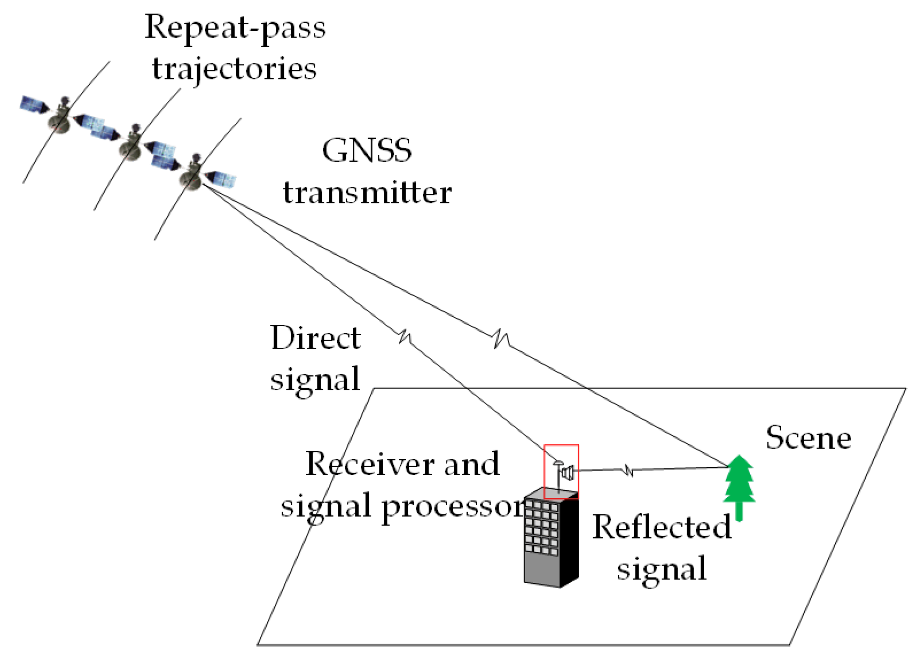
Figure 2.
Experimental scene. Beijing Institute of Technology, Haidian District, Beijing (39°57′22.84″ N, 116°18′47.59″ E).
Figure 2.
Experimental scene. Beijing Institute of Technology, Haidian District, Beijing (39°57′22.84″ N, 116°18′47.59″ E).

Figure 3.
The flowchart of the deformation retrieval processing.

Figure 4.
Experiment data collection strategy of GNSS-based InSAR.

Figure 5.
Spatial decoherence compensation results based on the proposed method: (a) spatial coherence coefficient; (b) phase noise.
Figure 5.
Spatial decoherence compensation results based on the proposed method: (a) spatial coherence coefficient; (b) phase noise.

Figure 6.
Comparison of radar imaging results and optical images: (a) the result of IGSO1 satellite; (b) the result of IGSO2 satellite; (c) the result of IGSO4 satellite.
Figure 6.
Comparison of radar imaging results and optical images: (a) the result of IGSO1 satellite; (b) the result of IGSO2 satellite; (c) the result of IGSO4 satellite.

Figure 7.
PS points distribution under threshold 0.2 of three IGSO satellites. (a–c) are the PS points selection results of IGSO 1, 2 and 4 satellites.
Figure 7.
PS points distribution under threshold 0.2 of three IGSO satellites. (a–c) are the PS points selection results of IGSO 1, 2 and 4 satellites.

Figure 8.
Multi-angle PS point association diagram.

Figure 9.
Lidar image of the target area. DEM information can be obtained through the lidar result.

Figure 10.
Extracted inter-channel phase error and compensation results: (a) interferometric phase at the origin point; (b) interferometric phase of Gym before inter-channel phase error compensation; (c) interferometric phase of Gym after inter-channel phase error compensation; (d) interferometric phase of Building 1 before inter-channel phase error compensation; (e) interferometric phase of Building 1 after inter-channel phase error compensation.

Figure 11.
Residual phase of the transponder from three IGSO satellites and the average residual phase.
Figure 11.
Residual phase of the transponder from three IGSO satellites and the average residual phase.

Figure 12.
Interferometric phase after compensation of typical buildings: (a) the compensation result of Gym; (b) the compensation result of Building 1.
Figure 12.
Interferometric phase after compensation of typical buildings: (a) the compensation result of Gym; (b) the compensation result of Building 1.

Figure 13.
Estimated deformations with transponder displacement in all directions: (a) the result along the upward direction; (b) the result along east and north directions.
Figure 13.
Estimated deformations with transponder displacement in all directions: (a) the result along the upward direction; (b) the result along east and north directions.

Figure 14.
The residual phase error of the transponder: (a) the result of the previous experiment; (b) the result of the proposed experiment.
Figure 14.
The residual phase error of the transponder: (a) the result of the previous experiment; (b) the result of the proposed experiment.


Table 1.
Repeat-pass period statistics of Beidou-2 satellite.
| Type | IGSO | MEO |
|---|---|---|
| Nominal repeat-pass period | 23 h 56 min 0 s (1 sidereal day) | 6 d 23 h 32 min 0 s (7 sidereal days) |
| Real repeat-pass period | 23 h 55 min 56–59 s | 6 d 23 h 31 min 40–44 s |
Table 2.
System parameters.
| Parameter | Value |
|---|---|
| Nominal repeat-pass cycle | 1 sidereal day |
| Carrier frequency | 1268.52 MHz (B3I) |
| Wavelength | 0.2365 m |
| Transmitted signal | C/A code |
| Effective signal bandwidth | 10.23 MHz |
| Equivalent PRT | 1 ms |
| Orbit height | About 36,000 km |
| Horn antenna gain | 11 dB |
| Horn antenna main lobe width |
Table 3.
Space decoherence compensation results for Beidou IGSO1.
| Interference Pair | Interference Pair | ||
|---|---|---|---|
| M01, M02 | 7.636 s | M09, M10 | 3.681 s |
| M02, M03 | −1.863 s | M10, M11 | 4.681 s |
| M03, M04 | 2.335 s | M11, M12 | 8.354 s |
| M04, M05 | 1.101 s | M12, M13 | 17.108 s |
| M05, M06 | −7.873 s | M13, M14 | 11.199 s |
| M06, M07 | 2.552 s | M14, M15 | 4.325 s |
| M07, M08 | −6.231 s | M15, M16 | 5.432 s |
| M08, M09 | 7.198 s | M16, M17 | 2.135 s |
Table 4.
of different targets.
| Target | Transponder | Building 1 | Gym |
|---|---|---|---|
| 172 m | 216 m | 410 m |
Table 5.
Deformation retrieval results of the typical buildings from ground-based SAR system.
| Building 1 | Gym | |
|---|---|---|
| Deformation value | 0.57 mm | 0.42 mm |
| Accuracy | 1.33 mm | 1.32 mm |
Table 6.
Deformation retrieval accuracy results of the typical buildings from a GNSS-based system.
| Gym | |||
|---|---|---|---|
| IGSO1 | IGSO2 | IGSO4 | |
| Traditional PS-InSAR processing | 20.94 mm | 18.34 mm | 28.11 mm |
| Proposed PS-InSAR processing | 10.61 mm | 11.64 mm | 17.26 mm |
| Building 1 | |||
| IGSO1 | |||
| Traditional PS-InSAR processing | 24.03 mm | ||
| Proposed PS-InSAR processing | 15.82 mm | ||
Table 7.
Deformation values of the typical buildings from GNSS-based system.
| IGSO1 | IGSO2 | IGSO4 | |
|---|---|---|---|
| Gym | −4.66 mm | −5.21 mm | −3.33 mm |
| Building 1 | −1.23 mm |
Table 8.
The accuracy of the deformation retrieval of the transponder.
| Direction | RMSE (mm) |
|---|---|
| East | 1.68 |
| North | 2.82 |
| Up | 4.22 |
Publisher’s Note: MDPI stays neutral with regard to jurisdictional claims in published maps and institutional affiliations. |
© 2021 by the authors. Licensee MDPI, Basel, Switzerland. This article is an open access article distributed under the terms and conditions of the Creative Commons Attribution (CC BY) license (https://creativecommons.org/licenses/by/4.0/).
Share and Cite
MDPI and ACS Style
Wang, Z.; Liu, F.; Zeng, T.; Wang, C. Interferometric Phase Error Analysis and Compensation in GNSS-InSAR: A Case Study of Structural Monitoring. Remote Sens. 2021, 13, 3041. https://doi.org/10.3390/rs13153041
AMA Style
Wang Z, Liu F, Zeng T, Wang C. Interferometric Phase Error Analysis and Compensation in GNSS-InSAR: A Case Study of Structural Monitoring. Remote Sensing. 2021; 13(15):3041. https://doi.org/10.3390/rs13153041
Chicago/Turabian StyleWang, Zhanze, Feifeng Liu, Tao Zeng, and Chenghao Wang. 2021. "Interferometric Phase Error Analysis and Compensation in GNSS-InSAR: A Case Study of Structural Monitoring" Remote Sensing 13, no. 15: 3041. https://doi.org/10.3390/rs13153041
Note that from the first issue of 2016, this journal uses article numbers instead of page numbers. See further details here.