Article

Use of TanDEM-X and SRTM-C Data for Detection of Deforestation Caused by Bark Beetle in Central European Mountains

1
Department of Spatial Sciences, Faculty of Environmental Sciences, Czech University of Life Sciences Prague, Kamýcká 129, 16500 Praha-Suchdol, Czech Republic
2
Department of Forest Resources Management, Faculty of Forestry, University of Agriculture in Krakow, Al. 29 Listopada 46, 31-425 Krakow, Poland
3
Department of Nature Protection, Šumava National Park administration, Sušická 339, 34192 Kašperské Hory, Czech Republic
*
Author to whom correspondence should be addressed.
Remote Sens. 2021, 13(15), 3042; https://doi.org/10.3390/rs13153042
Submission received: 18 June 2021 / Revised: 27 July 2021 / Accepted: 28 July 2021 / Published: 3 August 2021

Abstract

:
The availability of global digital elevation models (DEMs) from multiple time points allows their combination for analysing vegetation changes. The combination of models (e.g., SRTM and TanDEM-X) can contain errors, which can, due to their synergistic effects, yield incorrect results. We used a high-resolution LiDAR-derived digital surface model (DSM) to evaluate the accuracy of canopy height estimates of the aforementioned global DEMs. In addition, we subtracted SRTM and TanDEM-X data at 90 and 30 m resolutions, respectively, to detect deforestation caused by bark beetle disturbance and evaluated the associations of their difference with terrain characteristics. The study areas covered three Central European mountain ranges and their surrounding areas: Bohemian Forest, Erzgebirge, and Giant Mountains. We found that vertical bias of SRTM and TanDEM-X, relative to the canopy height, is similar with negative values of up to −2.5 m and LE90s below 7.8 m in non-forest areas. In forests, the vertical bias of SRTM and TanDEM-X ranged from −0.5 to 4.1 m and LE90s from 7.2 to 11.0 m, respectively. The height differences between SRTM and TanDEM-X show moderate dependence on the slope and its orientation. LE90s for TDX-SRTM differences tended to be smaller for east-facing than for west-facing slopes, and varied, with aspect, by up to 1.5 m in non-forest areas and 3 m in forests, respectively. Finally, subtracting SRTM and NASA DEMs from TanDEM-X and Copernicus DEMs, respectively, successfully identified large areas of deforestation caused by hurricane Kyril in 2007 and a subsequent bark beetle disturbance in the Bohemian Forest. However, local errors in TanDEM-X, associated mainly with forest-covered west-facing slopes, resulted in erroneous identification of deforestation. Therefore, caution is needed when combining SRTM and TanDEM-X data in multitemporal studies in a mountain environment. Still, we can conclude that SRTM and TanDEM-X data represent suitable near global sources for the identification of deforestation in the period between the time points of their acquisition.

1. Introduction

In the last decades, computers and remote sensing drove innovations in Earth surface observation. Data availability has been continuously growing, including surface observation data at a variety of scales [1]. Synthetic Aperture Radar (SAR) sensors are commonly used for mapping Earth’s surface, particularly due to their capability of mapping large areas within a short time and due to the fact that they are almost independent of weather conditions (i.e., they penetrate clouds, smoke, fog, and rain). Several SAR satellite systems have been operating in the last two decades [2]. SAR sensors were, for example, on board the Space Shuttle Endeavour in 2000 (Shuttle Radar Topography Mission; [3]) as well as on board the TerraSAR-X and TanDEM-X satellites, which were launched in 2007 and 2010, respectively (TanDEM-X mission; [4]). The main aim of those missions was to create a global (or near-global in the case of SRTM) digital elevation model (DEM) of the Earth’s surface. The resulting models (i.e., SRTM DEM, NASA DEM, TanDEM-X DEM and Copernicus DEM) were made freely available and have become an essential source of Earth’s surface information, widely used, among others, in forestry [5], ecology [6,7], archaeology [8], and hydrology [9,10].
The radar signals with short wavelengths, such as the ones used for TanDEM-X and SRTM measurements, are unable to reach the bare ground due to the presence of above-ground objects (e.g., trees). In forested areas, therefore, the DEMs elevations derived from X- or C-band interferometric SAR returns correspond to the height of vegetation, while in the bare, vegetation-free landscape, they represent ground heights (but see [11] for automated estimation of forest height and underlying topography using TanDEM-X data). What can be considered unwanted bias in some applications (i.e., hydrological applications requiring bare ground), can be viewed as an exploitable signal in others, such as acquisition of forest canopy height [12,13,14,15,16].
Producing continuous maps of vegetation height, biomass, and detection of vegetation changes (e.g., deforestation) is a long-standing goal of remote sensing [12,17]. Using 3D data from different time points to identify the decrease in canopy height is a promising remote sensing approach to detect deforestation. Airborne laser scanning (ALS) is the method best suited to produce such maps [18]. However, ALS surveys are costly and repeated surveys of large areas are rare, which limits their usability for large-scale detection of vegetation changes (but see [19,20]). There is, therefore, a demand for methods that enable more frequent repetition. One possible solution could lie in the utilization of methods based on SAR data that are increasingly being proposed as useful for detecting vegetation changes (e.g., for estimation of forest degradation or growth) caused by human activities or natural phenomena [21,22,23]. Vegetation changes can be detected using data from a single sensor [24,25] or using a combination of data from multiple sensors (e.g., of TanDEM-X acquired between 2011 and 2015 and SRTM DEM acquired in 2000). However, the accuracy of such estimates is limited, as combining multiple DEMs increases the risk and magnitude of errors (see Table 1 for recent studies that validated TanDEM-X DEM or compared it with other existing global DEMs); hence, potential sources of error in such analyses need to be properly investigated [26].
Disturbance are a natural part of the forest dynamics [27]. In the last decades, disturbances have increased in terms of both quantity and intensity in Central European forest. Strong winds, and subsequent bark beetle (Ips typographus) outbreaks are the most common type of disturbances in the Norway spruce forest [28] (the representation of which in the Czech mountain forests is dominant), which triggered intensive research in the field of remote sensing methods for early detection of bark beetle activity as well as for damage monitoring [29,30,31,32,33]. Between 2008 and 2011, after Hurricane Kyrill in 2007, the Bohemian Forest in Czechia went through a massive bark beetle outbreak, which resulted in a large-scale dieback of the natural mountain spruce forest (in high elevations > 1150 m a.m.s.l.). For this area, severe disturbances (>50% trees affected) with a short rotation period of 174 years are common [34]. However, with increasing temperatures and reduced precipitation resulting from global warming, the number of possible bark beetle generations per year and their survival through winter periods keep increasing. In addition, global warming also reduces the vitality of trees, negatively affecting their ability to resist an attack. We can, therefore, expect an increase in the number and severity of bark beetle outbreaks in the near future [35,36,37] and detecting their impact through remote sensing techniques can be a great help for forest managers.
The main objective of this study was to examine the suitability of the combination of SRTM and TanDEM-X data for the detection of such large deforestation and to identify potential sources of error. The nature of DEM errors constantly attracts extensive attention and recent studies evaluating the accuracy of TanDEM-X DEM highlighted that it is superior to other DEMs and emphasized the improvement in detail in TanDEM-X DEM compared to other global DEMs (see Table 1). Here, we aim to (i) compare the SRTM and TanDEM-X at 90 m resolution with a LiDAR-based DSM to evaluate their performance as DSMs in forests and non-forested areas; (ii) evaluate the associations of the differences between SRTM and TanDEM-X with terrain slope and orientation (i.e., assess a potential synergy of errors in both models that may affect the detection of deforestation); and (iii) compare the detected differences with local data and with the Global Forest Change 2000–2012 data produced by Hansen et al., (2013) [38].

2. Data and Methods

2.1. Study Areas and Reference Data

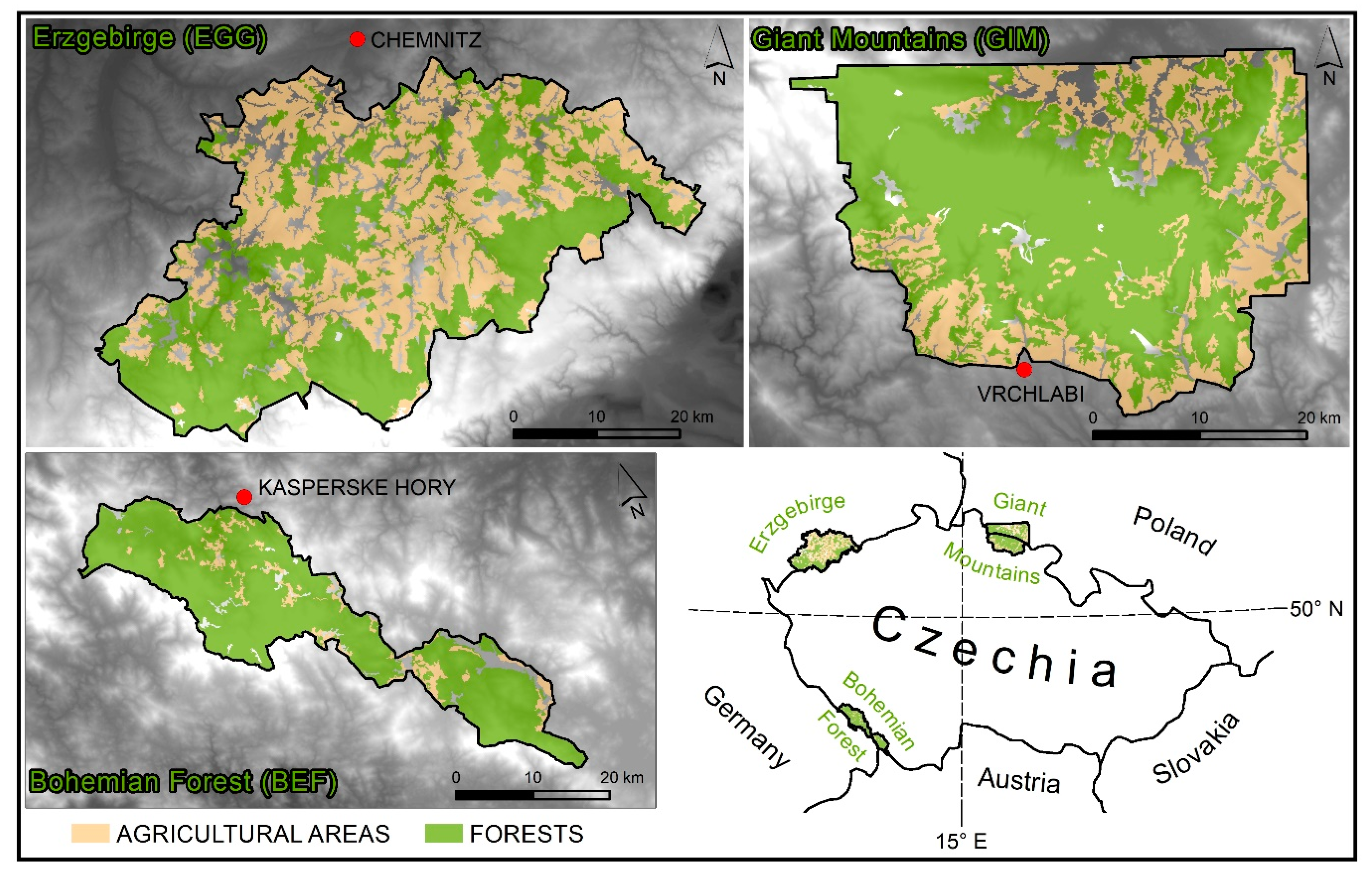
To assess the suitability of space-borne DEMs for vegetation change analysis, they were first compared with existing high-resolution LiDAR-based DSMs in three study areas. The study areas representing mountain environment were selected on the basis of the LiDAR data availability, comprising three Central European mountain ranges and their surrounding areas (Figure 1): Bohemian Forest (BEF), Erzgebirge (EGG), and Giant Mountains (GIM). The study areas are situated in Germany, Czechia, and Poland with altitudes ranging between 300 and 1600 m a.m.s.l, covering about 920 km2 (Bohemian Forest), 1840 km2 (Erzgebirge), and 1200 km2 (Giant Mountains), respectively. The basic specifications of the LiDAR data acquisitions are shown in Table 2.

2.1.1. Bohemian Forest

The airborne LiDAR data for the Bohemian Forest study area were collected by MILAN GeoService GmbH in June 2017 during a leaf-on period, using the Riegl LMSQ680i scanner. Flights for data collection were conducted by a helicopter at 550 m above ground at a velocity of 60 kts and with 60% flight line side overlap. The obtained LiDAR point cloud density is 55 points per m2. The LiDAR point cloud was processed by MILAN GeoService GmbH and provided as DTM and DSM referenced to DHDN/3-degree Gauss–Kruger zone 4 coordinate reference system (EPSG: 31468), and with elevation recorded as orthometric heights.

2.1.2. Erzgebirge

The DTM and DSM of Erzgebirge was provided by “Staatsbetrieb Geobasisinformation und Vermessung Sachsen (GeoSN)” as open data under the dl-de/by-2-0 license. The airborne LiDAR data for Saxony were collected between 2015 and 2017. The LiDAR point cloud density is at least 4 points per m2. The data were downloaded as a DTM and DSM, respectively, with a resolution of 2 m. The height accuracy of the terrain models from the laser scanner measurements was up to +/−0.15 m and the positional accuracy up to +/−0.3 m. The horizontal coordinates use ETRS89 UTM33N zone (EPSG: 25833) and the vertical coordinate uses the “DHHN2016” (EPSG: 7837).

2.1.3. Giant Mountains

The airborne LiDAR data for the Czech part of the Giant Mountains study area were collected in 2012. The data were acquired during the leaf-on period, using a Riegl LMSQ680i scanner. Flights for the data collection were conducted at 700 m above ground and consisted of 553 flight lines with an approximately 20% flight line side overlap. The obtained LiDAR point cloud density was 5 points per m2. We classified the point cloud into the ground, vegetation, building, wire, and transmission tower classes in the ENVI LiDAR software (version 5.3) and LAStools (version 171215), and produced DTM and DSM at a 1 m resolution [50,51]. The vertical datum of the LiDAR point cloud is Baltic Vertical Datum—after adjustment (EPSG: 5705), and the horizontal datum is the Datum of Uniform Trigonometric Cadastral Network (EPSG: 5514).
The airborne LiDAR data for the Polish part of the Giant Mountains study area were collected during the nationwide project- IT System for the Country’s Protection project (pl. “Informatyczny System Osłony Kraju”; ISOK project) managed by the Main Office of Geodesy and Cartography in Poland. The project aimed mainly at creating a detailed digital terrain model for the whole of Poland. The data were acquired in 2011–2015 and referenced to Poland CS92 (EPSG: 2180). The vertical datum of the LiDAR point cloud was the Mean Sea Level (MSL; PL-KRON86-NH). The point cloud density was at least four pulses per square meter with an altitude accuracy of ≤0.15 m. Generally, the acquisition of ALS point clouds took place from mid-October to April (i.e., in the leaf-off period, which guaranteed good penetration of the laser beams through the forest stand. However, for the Polish Giant Mountains area, data acquisition was performed in the leaf-on period (from April to October). The data were collected in three blocks: two of them with density 4 points/m2 (collecting period: 11 April–20 October 2012) and one with 12 points/m2 (collecting period: 18 June–8 July 2012).

2.1.4. Land Cover Data

We obtained land cover data for both years from the Corine land cover database with a resolution of 100 m. Only areas that were classified as agricultural areas or forests both in 2000 and 2012, respectively (i.e., no land cover change), were used in the study (note that natural disturbances or logging are not recorded as a land cover change as such areas remain classified as forests). The land cover of our study areas consists mostly of agricultural areas and forests (hereafter non-forests and forests; Table 2; Figure 1). Note that no terrain changes occurred between SRTM and TanDEM-X DEMs acquisitions in the study areas.

2.2. Global DEMs (TanDEM-X, Copernicus DEM, SRTM, NASADEM)

The free version of TanDEM-X DEM at the resolution of 90 m (3 arc-seconds) became available in 2018 (hereinafter, this version will be abbreviated as TDX90). Although TanDEM-X products are also available at 12 and 30 m resolutions, this option is only for scientific use; for general purposes, TanDEM-X is freely available only at a resolution of 90 m. Data used for the production of TanDEM-X products were collected by a constellation of two satellites using an X-band radar (TerraSAR-X and TanDEM-X) between 2010 and 2015 [52]. Nominal TanDEM-X acquisitions were performed in the right-looking observation mode, during ascending orbits in the Northern Hemisphere, and a combination of several acquisitions was used for most of the land [39]. The target absolute vertical accuracy is specified to be better than 10 m (90% linear error) [52]. The horizontal datum and vertical heights of the TDX90 are referenced to WGS84-G1150. The present version of TDX90 (version 1) is the final official standard non-edited product. Nevertheless, with the exception of two pixels in the Giant Mountains, which were removed for the purpose of this study, no voids were present in the TanDEM-X 90m DEM in our study areas. The TanDEM-X 90 m DEM was downloaded from https://download.geoservice.dlr.de/TDM90/ (accessed on 18 February 2021).
The SRTM raw data were collected using a C-band radar during an 11-day mission in February 2000 and captured the surface of the Earth between the 60° N and 56° S latitudes [3]. The goal was to record each terrain segment at least twice from different angles (on ascending and descending orbit passes) to fill the areas shadowed from the radar signal by terrain. SRTM DEM was first released in June 2003 and since then, it became one of the most commonly used global DEMs. The theoretical vertical accuracy according to the SRTM mission specifications is 16 m. However, studies generally report much better accuracies [53]. Co-registration with the TanDEM-X data was not carried out, as the SRTM-C was already used during initial processing steps to provide elevation corrections [52]. The horizontal datum for SRTM is WGS84 and the vertical datum is the EGM96 geoid. We downloaded the void-filled version SRTM DEM v3 with a resolution of 3 arc-seconds (i.e., the same resolution as TDX90 DEM; hereafter SRTM) from the Earth Explorer.
For the final detection of deforested areas in Bohemian Forest at 30 m resolution, we used also the Copernicus DEM and NASA DEM. Copernicus DEM is an edited (i.e., voids were filled and artefacts such as spikes and wells removed) DEM derived from TanDEM-X data, freely available at a 30 m resolution since the beginning of 2021 [54]. The vertical datum for Copernicus DEM is EGM2008 geoid and the horizontal datum is WGS84. NASA DEM is a modernization of the SRTM released in 2020, which results from complete re-processing of the raw radar echo and telemetry, and removal of large-scale systematic biases and void reductions [55]. Note that we did not adopt these two DEMs for all study areas as, particularly in the Giant mountains, many cells in Copernicus DEM were infilled by external—mainly SRTM—elevation data, making the comparison meaningless. The infill by external data was, however, minimal in the Bohemian Forest study area and after removal of such cells, the Copernicus DEM was ready for analysis. Potential users should be aware that using edited DEMs such as Copernicus or NASA DEM for multi-temporal analysis requires careful examination of auxiliary data, especially Editing Mask and Filling Mask [54].

2.3. Horizontal and Vertical Datum Conversion

To match the horizontal datum of the space-borne DEMs and reference LiDAR models, we took advantage of the fact that study areas fit into a single UTM zone and transformed all models using the bilinear resampling method into WGS84 UTM33N at a 90 m resolution. LiDAR models were first transformed using the bilinear resampling method and subsequently aggregated to the same resolution as the space-borne DEMs. The vertical datum of all datasets is represented as orthometric heights except for the TDX90, which represents ellipsoidal heights. In order to match the ellipsoidal heights of TDX90 with the orthometric heights of other models, we used a quasigeoid of Czechia and surrounding areas (grid of latitude/longitude coordinates at 1’ × 1.5’ resolution).

2.4. Accuracy Assessment

To assess the absolute vertical accuracy of a DEM, an independent reference dataset is needed. Here, we compared the height of individual global DEMs with ALS-derived DSMs. The accuracy of the reference data should be at least three times better than the evaluated DEM [56]. As mentioned above, the target absolute vertical accuracies specified as LE90 for the TDX90 and SRTM DEMs validated in this study were better than 10 m and 16 m, respectively. This implies a required LE90 error of 3.3 m for the reference LiDAR DSMs, leading to the required standard deviation being lower than 2 m. This requirement is easily met by ALS data, the typical accuracies of which are in the range of several decimetres [57].
To assess the vertical difference between global DEMs and canopy height, we calculated height differences between the reference LiDAR DSM and the global DEMs. To assess the absolute vertical accuracy of TDX90 and SRTM DEMs with respect to the vegetation cover, we calculated the accuracy measures separately for non-forests and forests. We plotted the density distribution of height differences and used the differences to calculate root mean square error (RMSE), the absolute deviation at 90% quantile (LE90), and mean error (ME), expressed as:
M E = 1 n i = 1 n ( h D E M i h R E F i ) = 1 n i = 1 n Δ h i
R M S E = 1 n i = 1 n Δ h i 2
L E 90 = Q | Δ h | ( 0.9 )
where n is the total number of sampled cells, hDEMi is the ith height from the global DEM, and hREFi is the corresponding height from the LiDAR DSM. LE90 was calculated as the 90th percentile of manually sorted absolute height differences (i.e., 90% of the differences are less than or equal to this value) [58].

2.5. Detection of Deforestation and Validation of Results

The acquisition of TanDEM-X and SRTM data was performed at different time points and their combination is now increasingly used for the assessment of vegetation changes [59,60]. Data for SRTM were acquired in February 2000 while TanDEM-X data were acquired over a four-year period between December 2010 and January 2015. In the meantime, Bohemian Forest has gone through a bark beetle disturbance with major deforestation between 2008 and 2011 after Hurricane Kyrill in 2007 [61]; ca. six thousand hectares of mature mountain spruce forest died during this period. Therefore, to evaluate whether the degree of such forest loss can be accurately derived from global DEMs, we subtracted the SRTM and NASA DEMs from the TDX90 and Copernicus DEMs, respectively, visually assessed the differences, and compared it with two validation datasets: (i) a polygon layer provided by the Šumava National Park administration (area of Bohemian forest), which is based on field surveys and high-resolution orthophoto images, showing an annual forest loss between 2006 and 2020. Each polygon is in a given year assigned to one of the following categories (no change; standing dead trees; lying dead trees; salvage logging, windfalls); and (ii) the Global Forest Change 2000–2012 data derived from Landsat images at 30 m resolution. In particular, we used the forest cover loss dataset defined as a change from forest to non-forest state (note that forests are defined as vegetation taller than 5 m) [38,62]. In addition, we evaluated the effect of environmental conditions on the magnitude of SRTM and TDX90 differences. We assessed the effect of the terrain character using the slope and aspect. The terrain slope and aspect were derived from a LiDAR DTM at a 90 m resolution (i.e., we first aggregated the LiDAR DTM to a 90 m resolution using mean values and then calculated the terrain characteristics) [63,64]. We used the Horn’s algorithm with a 3 × 3 cell neighbourhood implemented in ArcGIS (version 10.8.1) [65].

3. Results

3.1. Comparison of SRTM and TDX90 with LiDAR-Based DSM

In non-forest areas, the density plots of height differences between the global models and LiDAR-based DSM show a symmetric unimodal distribution with the distribution maxima close to zero (Figure 2). Although RMSEs in non-forest areas are similar, i.e., below 4.5 m, for both models (Table 3), TDX90 shows a considerably narrower spread of height differences than SRTM in all study areas. In forests, the RMSE of TDX90 is below 5.7 m while that of SRTM ranges between 5.2 and 7.3 m. The density plots of canopy height differences show a unimodal distribution with the centre of the distribution shifted into the negative values. This is particularly true for SRTM DEM while for TDX90 DEM, the distribution maximum is closer to zero (i.e., both models underestimate the canopy height on average by a few meters; Table 3). The vegetation height underestimation is slightly higher in the case of SRTM (except for forests in the BEF study area).

3.2. Associations of Difference between TDX90 and SRTM with Terrain Characteristics

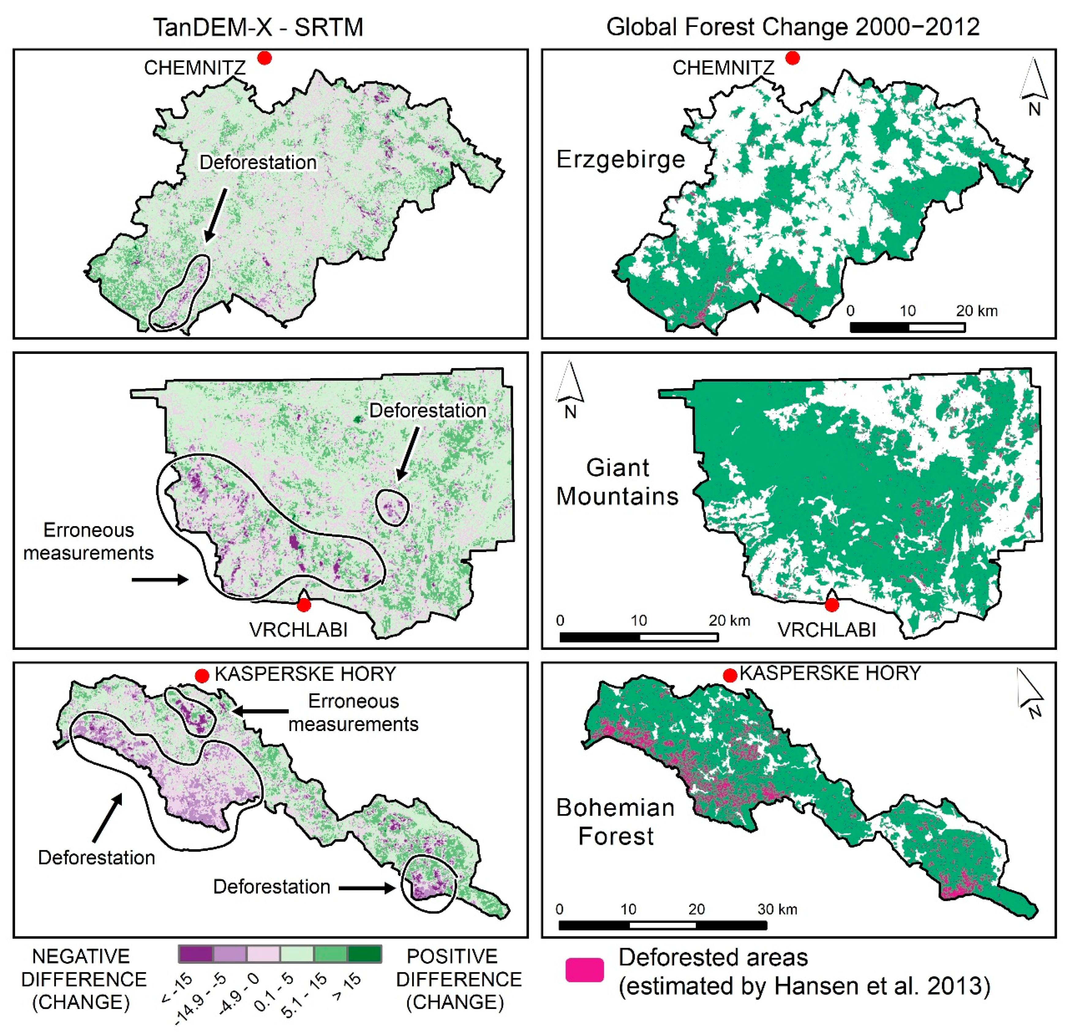
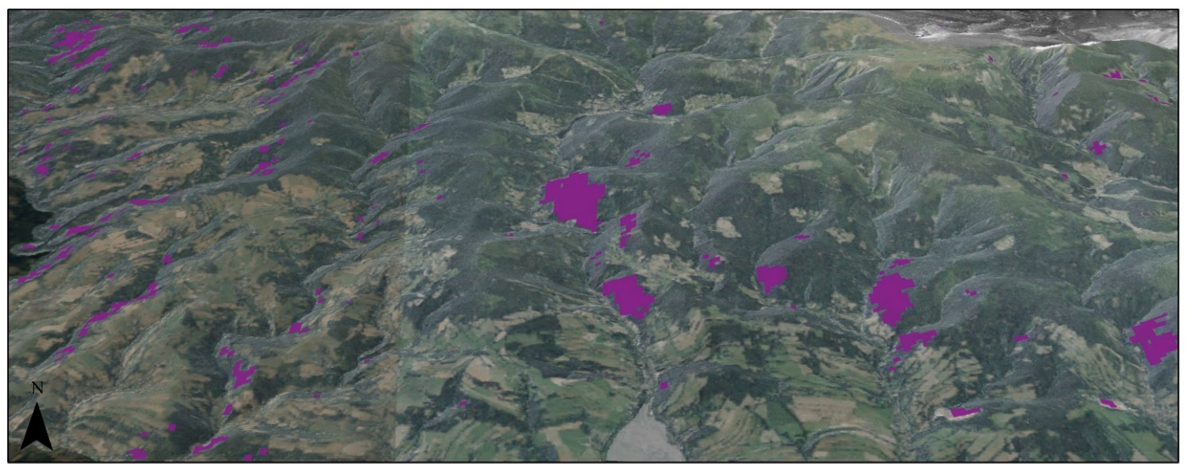
We evaluated the associations of the difference between TDX90 and SRTM with terrain characteristics (Table 4). Under optimal circumstances (i.e., if no erroneous measurements were present), we should observe positive or negative bias in forest areas (depending on the vegetation growth or removal in the period between the acquisitions of these models) and no bias in non-forest areas. Indeed, our results show only minor differences between TDX90 and SRTM in both non-forest areas (mean difference of 0.4 m) and forests (mean difference of 1.3 m). In non-forest areas, the RMSE of the differences between TDX90 and SRTM was 2.0 m; in forests, RMSE was slightly higher, namely 5.6 m (Table 4). The overall characteristics were moderately associated with the terrain character. Height differences show slight dependence on the slope and its orientation. LE90s for TDX-SRTM differences tended to be smaller for east-facing than west-facing slopes, and vary with aspect by up to 1.5 m in non-forest areas and 3 m in forests, respectively (Table 4). This corresponds with visual assessment of TDX90 and SRTM difference, which revealed high local negative differences between TDX90 and SRTM originating from erroneous TDX90 measurements especially on west-facing slopes with forest cover (Figure 3 and Figure 4). The comparison of TDX90 with canopy height represented by SRTM (Figure 3; left column) demonstrates a local underestimation of the canopy height. In effect, the errors in the GIM study area (Figure 3 and Figure 4) can easily be confused with the effect of deforestation in the BEF study area (Figure 3), which can potentially affect vegetation change analyses.

3.3. Detection of Deforestation in the Bohemian Forest

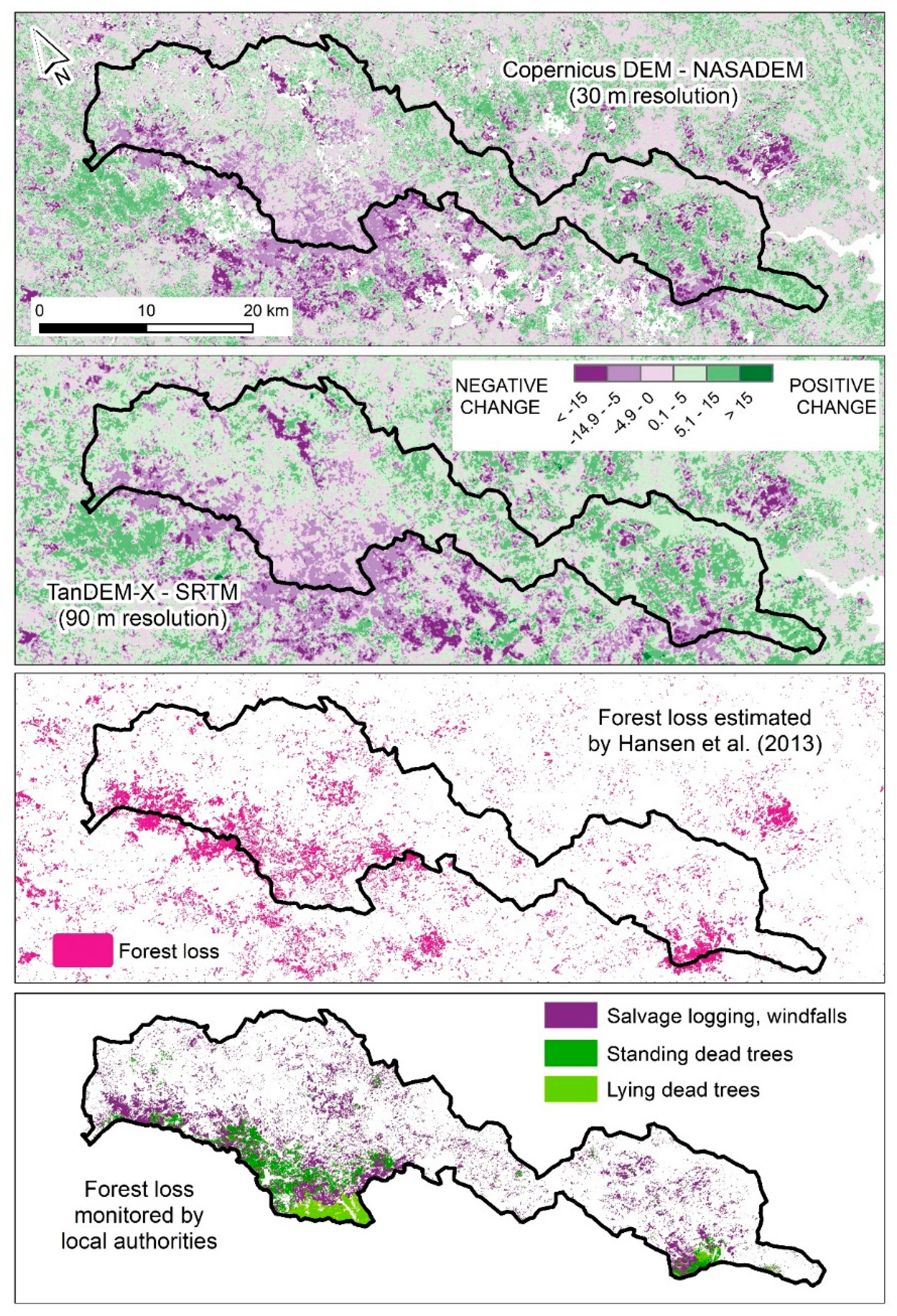
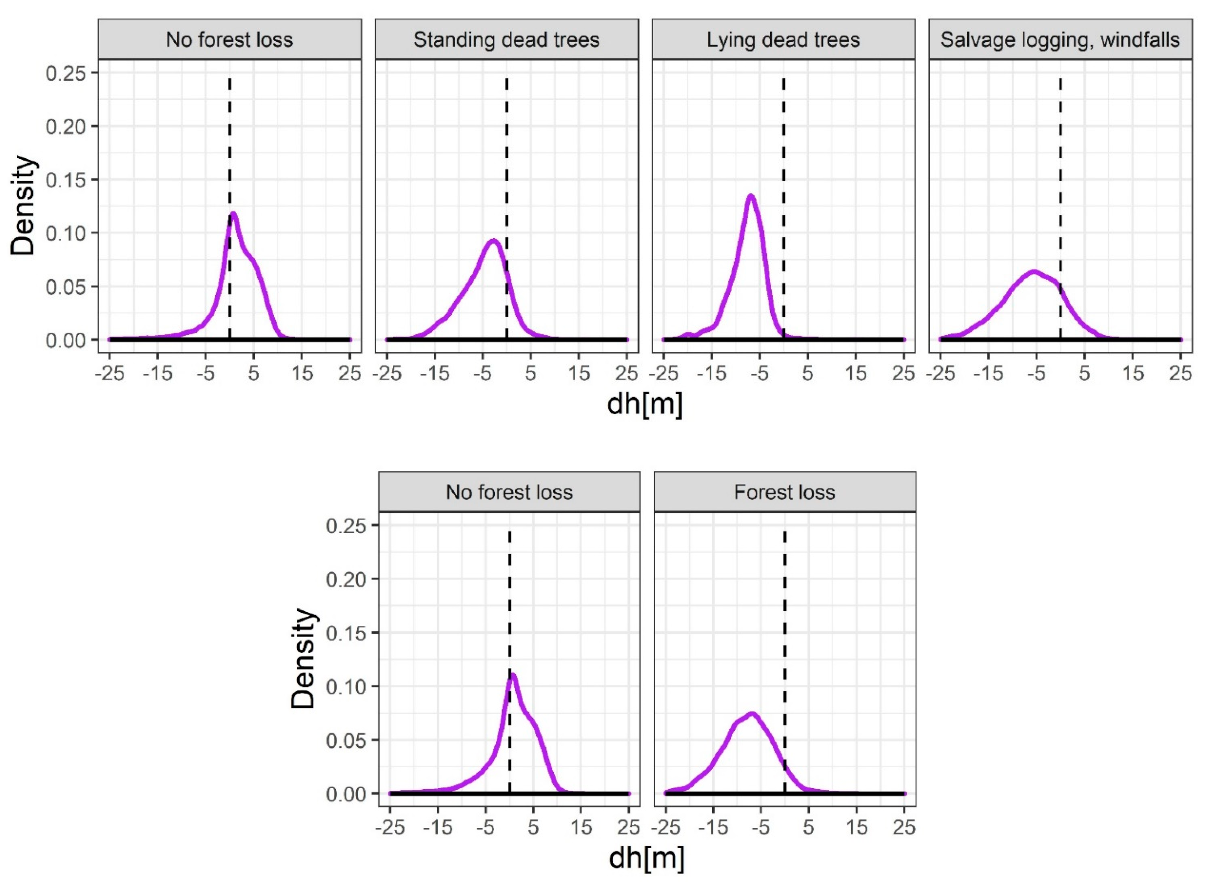
We subtracted the SRTM and TanDEM-X at the 90 m resolution, and NASA DEM and Copernicus DEM at the 30 m resolution, respectively, in an attempt to detect deforestation events occurring in the Bohemian Forest in the period between their acquisitions (2000–2011). Negative difference was considered a sign of deforestation/degradation while a positive difference was considered a sign of forest growth or afforestation. The comparison with validation datasets showed a clear correspondence between the spatial pattern of negative changes and deforested areas in the Bohemian Forest. Negative changes in canopy height are visualized in purple while positive changes in green (Figure 5). It is notable that the deforestation is so extensive that the overall pattern is clearly evident even at the 90 m resolution. In addition, forest loss in the “lying dead trees” category was inadequately identified in the Global Forest Change 2000–2012 data (i.e., using Landsat multispectral data), while our approach using 3D data identified it correctly (Figure 5). The density plots of canopy height differences show a unimodal distribution with the distribution shifted either into the positive values (in areas without forest loss) or into negative values (in deforested areas—standing or lying dead trees as well as areas with salvage logging). The same pattern is evident for the Global Forest Change 2000–2012 data (Figure 6).

4. Discussion

In this study, we showed that large deforestation can be successfully identified from global DEMs difference. We successfully identified deforestation in the Bohemian Forest caused by the bark beetle disturbance between 2008 and 2010 (Figure 3). On the other hand, however, we also identified local erroneous measurements of deforestation (Figure 3) that were mostly associated with underestimation of the vegetation height by TDX90, mostly on the west-facing slopes (i.e., slopes facing the sensor; Figure 4). Our results show a moderate dependence of the differences between TDX90 and SRTM on terrain characteristics (i.e., slope and aspect), mostly with positive bias (Table 4). This is in accordance with results by Leonardo et al. (2020) [15] who also reported the deterioration of canopy height data derived from TanDEM-X with increasing slope. These errors might be easily confused with deforestation (Figure 3) and can locally affect its estimates. Most errors of this kind in our study were located in the Giant Mountains, representing the highest mountains with the most complex terrain of all analysed areas.
While this study concentrated on negative differences associated with deforestation, other studies used DEM differencing to estimate both positive and negative changes in vegetation height (or biomass) due to both forest degradation and/or forest growth [5,21,22]. However, large errors in the vegetation biomass estimates are typically reported, along with numerous issues related to input DEMs [26], and the in-depth knowledge of the accuracy of SRTM and TanDEM-X is necessary for the accurate detection of vegetation changes. Based on our results, we strongly suggest that prior to performing vegetation change analyses, potentially erroneous areas in global DEMs should be acknowledged. Problematic areas can be successfully identified using auxiliary data such as the consistency mask (COM), the coverage map (COV), and the height error map (HEM) provided together with TDX [40,46].
The target vertical accuracies stated in the specifications of SRTM and TDX90 (expressed as 90% of the product errors, LE90) should be below 16 and 10 m, respectively. Both SRTM and TDX90 comply with mission specifications when compared to LiDAR DSM. Our results show, despite the presence of local errors that may result in underestimation of canopy height (Figure 3 and Figure 4), that TDX90 yields a generally better fit to LiDAR-based DSM than SRTM. This difference was not so apparent in non-forest areas where similar differences from LiDAR-based DSM were found for both models (although TDX90 showed higher consistency of results and a considerably narrower spread of height differences than SRTM in all study areas). In forests, the better fit of TDX90 to DSM is even more pronounced, with the SRTM results being shifted to the negative values. However, it is necessary to point out that this result was expected, in particular, due to the large time difference between acquisitions of SRTM and TDX90; to be able to reliably evaluate the goodness of fit of the global DEMs to actual LiDAR-based DSMs, two LiDAR-based models from the times of global DEM acquisitions would be necessary.
Due to the limited data availability, it is a common practice of remote sensing applications in forestry to combine datasets from multiple time points. Our study is not an exception and the time of acquisition should be taken into account when interpreting the results. LiDAR data has been acquired a few years after the acquisition of TDX data, except for the Giant Mountains study area (Table 2). Consequently, the negative bias between TDX (and SRTM, respectively), and LiDAR DSM is not only the result of radar penetration into the vegetation but also vegetation growth. In addition, data may be generally acquired at a time of the year that is unsuitable for forestry applications (e.g., leaf-off period), which might lead to canopy height underestimation in such data (and, hence, have an opposite effect than vegetation growth). SRTM was acquired in February (winter in the northern hemisphere) in contrast to TDX, which is averaged from multiple acquisitions taken between December 2010 and January 2015. The forests in all study areas are, however, mainly coniferous and, therefore, we did not expect any significant underestimation of the canopy surface. This might have, however, resulted in an additional positive bias in the non-forested areas due to the presence of vegetation, such as crops on agricultural fields, during TDX data acquisition; such vegetation was not present in winter when SRTM was acquired. In forests, the positive bias also results from the lower X-band penetration into the vegetation compared to the C-band and, obviously, from the forest growth between the dates of SRTM and TDX data acquisition (i.e., 2000 and 2011).
The time of acquisition is also related to the presence/absence of snow cover, another environmental factor that might bias our results. In the winter months, the thickness of the snow cover in this region can easily reach several meters resulting in uncertainty due to the unknown penetration of the radar signal into the snow [66]. The level of penetration is dependent on the snow properties such as the content of the liquid water; while dry snow can potentially be penetrated by the X-band radar, the penetration into wet (i.e., containing liquid water) snow can be considered negligible [67]. However, as the study areas are predominantly forested by spruce stands, it is likely that this source of error is relatively minor in forested areas and does not affect the detection of deforestation.
Although the above mentioned facts considerably increase the uncertainty of the performed analyses, the results show that if there is a negative difference between TDX and SRTM, it can be inferred that deforestation has occurred in a given cell (Figure 6). In addition, the detection of deforestation may be improved by using various thresholds. Prior studies have adopted a threshold of −7 m for detecting deforested areas [59,60,68], which roughly corresponds to the distribution maximum of deforested areas height differences between Copernicus DEM and NASA DEM (Figure 6). In other words, looking at the data from Figure 6, it appears that the threshold of −7 m is justified as there are very few errors of more than −7 m in the “no forest loss” category that could be erroneously classified as forest loss. Finally, our approach using 3D data adequately identified forest loss in all assessed categories, while in the Global Forest Change 2000–2012 data (i.e., using Landsat multispectral data) the “lying dead trees” category was identified inadequately. Integration of multispectral and SAR data, which provide complementary information, can improve monitoring of forest loss.

5. Conclusions

In the present study, we evaluated two global DEMs produced using radar interferometry (SRTM and TanDEM-X) in three Central European mountain ranges. Models acquired using the same technology, such as SRTM and TanDEM-X, can be expected to be subject to similar errors. When combined, for example, for vegetation change assessments, these errors can have a synergistic effect and lead to erroneous results. A comparison of SRTM and TanDEM-X 90m DEM with LiDAR DSMs showed that both models tend to underestimate the canopy height by several meters. Our analysis shows that differences of SRTM and TanDEM-X show a moderate dependence on terrain characteristics. In particular, we found local errors in TanDEM-X associated mainly with forest-covered west-oriented slopes, which resulted in erroneous identification of canopy changes. Therefore, researchers should proceed with caution when using TanDEM-X in multitemporal studies. However, if these problems are acknowledged and their adverse effects prevented, the combination of SRTM and NASA DEMs and TanDEM-X and Copernicus DEMs, respectively, represents a suitable source for the identification of deforested areas in the mountain environment.

Author Contributions

Conceptualization, M.S. and V.M.; Data curation, K.G. and J.Č.; Formal analysis, V.B.; Funding acquisition, K.G., J.M. and J.Č.; Methodology, K.G. and V.M.; Project administration, K.G. and J.M.; Software, K.G. and J.M.; Supervision, V.M.; Visualization, J.M. and V.M.; Writing—original draft, K.G. and V.M.; Writing—review and editing, J.M., V.B., J.Č., M.S., K.G. and V.M. All authors have read and agreed to the published version of the manuscript.

Funding

The data acquisition was funded by the cross-border cooperation programme Czech Republic–Bavaria Free State ETC goal 2014–2020, the Interreg V project No. 99: Preshranicni mapovani lesnich ekosystemu—cesta ke spolecnemu managementu NP Šumava a NP Bavorsky les/Grenzuberschreitende Kartierung der Waldokosysteme–Weg zum gemeinsamen Management in NP Sumava und NP Bayerischen Wald’). This work was supported by the Internal Grant Agency of the Faculty of Environmental Sciences, Czech University of Life Sciences Prague (project no. 2020B0022) and by the Technological Grant Agency of the Czech Republic, grant no. SS02030018 DivLand.

Data Availability Statement

The data presented in this study are available on request from the corresponding author.

Acknowledgments

We are grateful to the administrations of the Krkonose Mountains National Park, Šumava National Park, and the Head Office of Geodesy and Cartography in Poland for providing the airborne laser scanning data. We also acknowledge Šumava National Park for providing data of forest loss. We also thank the “Staatsbetrieb Geobasisinformation und Vermessung Sachsen (GeoSN)” for providing access to the DTM of Saxony (https://www.geodaten.sachsen.de/digitale-hoehenmodelle-3994.html; accessed on 31 July 2021) as open data under the dl-de/by-2-0 license (https://www.govdata.de/dl-de/by-2-0; accessed on 31 July 2021).

Conflicts of Interest

The authors declare no conflict of interest.

References

  1. Koppes, M.; King, L. Beyond x, y, z (t). Navigating New Landscapes of Science in the Science of Landscapes. J. Geophys. Res. Earth Surf. 2020, 125, e2020JF005588. [Google Scholar] [CrossRef]
  2. Toth, C.; Jóźków, G. Remote Sensing Platforms and Sensors: A Survey. ISPRS J. Photogramm. Remote Sens. 2016, 115, 22–36. [Google Scholar] [CrossRef]
  3. Farr, T.G.; Rosen, P.A.; Caro, E.; Crippen, R.; Duren, R.; Hensley, S.; Kobrick, M.; Paller, M.; Rodriguez, E.; Roth, L. The Shuttle Radar Topography Mission. Rev. Geophys. 2007, 45. [Google Scholar] [CrossRef] [Green Version]
  4. Bojarski, A.; Bachmann, M.; Böer, J.; Kraus, T.; Wecklich, C.; Steinbrecher, U.; Ramon, N.T.; Schmidt, K.; Klenk, P.; Grigorov, C. TanDEM-X Long-Term System Performance after 10 Years of Operation. IEEE J. Sel. Top. Appl. Earth Obs. Remote Sens. 2021, 14, 2522–2534. [Google Scholar] [CrossRef]
  5. Hojo, A.; Takagi, K.; Avtar, R.; Tadono, T.; Nakamura, F. Synthesis of L-Band SAR and Forest Heights Derived from TanDEM-X DEM and 3 Digital Terrain Models for Biomass Mapping. Remote Sens. 2020, 12, 349. [Google Scholar] [CrossRef] [Green Version]
  6. Sesnie, S.E.; Gessler, P.E.; Finegan, B.; Thessler, S. Integrating Landsat TM and SRTM-DEM Derived Variables with Decision Trees for Habitat Classification and Change Detection in Complex Neotropical Environments. Remote Sens. Environ. 2008, 112, 2145–2159. [Google Scholar] [CrossRef]
  7. Kosicki, J.Z. Should Topographic Metrics Be Considered When Predicting Species Density of Birds on a Large Geographical Scale? A Case of Random Forest Approach. Ecol. Model. 2017, 349, 76–85. [Google Scholar] [CrossRef]
  8. Fanta, V.; Zouhar, J.; Beneš, J.; Bumerl, J.; Sklenicka, P. How Old Are the Towns and Villages in Central Europe? Archaeological Data Reveal the Size of Bias in Dating Obtained from Traditional Historical Sources. J. Archaeol. Sci. 2020, 113, 105044. [Google Scholar] [CrossRef]
  9. Hawker, L.; Neal, J.; Bates, P. Accuracy Assessment of the TanDEM-X 90 Digital Elevation Model for Selected Floodplain Sites. Remote Sens. Environ. 2019, 232, 111319. [Google Scholar] [CrossRef]
  10. Farooq, M.; Shafique, M.; Khattak, M.S. Flood Hazard Assessment and Mapping of River Swat Using HEC-RAS 2D Model and High-Resolution 12-m TanDEM-X DEM (WorldDEM). Nat. Hazards 2019, 97, 477–492. [Google Scholar] [CrossRef]
  11. Lei, Y.; Treuhaft, R.; Gonçalves, F. Automated Estimation of Forest Height and Underlying Topography over a Brazilian Tropical Forest with Single-Baseline Single-Polarization TanDEM-X SAR Interferometry. Remote Sens. Environ. 2021, 252, 112132. [Google Scholar] [CrossRef]
  12. Walker, W.S.; Kellndorfer, J.M.; Pierce, L.E. Quality Assessment of SRTM C- and X-Band Interferometric Data: Implications for the Retrieval of Vegetation Canopy Height. Remote Sens. Environ. 2007, 106, 428–448. [Google Scholar] [CrossRef]
  13. Kugler, F.; Schulze, D.; Hajnsek, I.; Pretzsch, H.; Papathanassiou, K.P. TanDEM-X Pol-InSAR Performance for Forest Height Estimation. IEEE Trans. Geosci. Remote Sens. 2014, 52, 6404–6422. [Google Scholar] [CrossRef]
  14. Schlund, M.; Magdon, P.; Eaton, B.; Aumann, C.; Erasmi, S. Canopy Height Estimation with TanDEM-X in Temperate and Boreal Forests. Int. J. Appl. Earth Obs. Geoinf. 2019, 82, 101904. [Google Scholar] [CrossRef]
  15. Leonardo, E.M.C.; Watt, M.S.; Pearse, G.D.; Dash, J.P.; Persson, H.J. Comparison of TanDEM-X InSAR Data and High-Density ALS for the Prediction of Forest Inventory Attributes in Plantation Forests with Steep Terrain. Remote Sens. Environ. 2020, 246, 111833. [Google Scholar] [CrossRef]
  16. Ullah, S.; Dees, M.; Datta, P.; Adler, P.; Saeed, T.; Khan, M.S.; Koch, B. Comparing the Potential of Stereo Aerial Photographs, Stereo Very High-Resolution Satellite Images, and TanDEM-X for Estimating Forest Height. Int. J. Remote Sens. 2020, 41, 6976–6992. [Google Scholar] [CrossRef]
  17. Rodríguez-Veiga, P.; Quegan, S.; Carreiras, J.; Persson, H.J.; Fransson, J.E.S.; Hoscilo, A.; Ziółkowski, D.; Stereńczak, K.; Lohberger, S.; Stängel, M.; et al. Forest Biomass Retrieval Approaches from Earth Observation in Different Biomes. Int. J. Appl. Earth Obs. Geoinf. 2019, 77, 53–68. [Google Scholar] [CrossRef]
  18. Nilsson, M.; Nordkvist, K.; Jonzén, J.; Lindgren, N.; Axensten, P.; Wallerman, J.; Egberth, M.; Larsson, S.; Nilsson, L.; Eriksson, J.; et al. A Nationwide Forest Attribute Map of Sweden Predicted Using Airborne Laser Scanning Data and Field Data from the National Forest Inventory. Remote Sens. Environ. 2017, 194, 447–454. [Google Scholar] [CrossRef]
  19. Yu, X.; Hyyppä, J.; Kaartinen, H.; Maltamo, M. Automatic Detection of Harvested Trees and Determination of Forest Growth Using Airborne Laser Scanning. Remote Sens. Environ. 2004, 90, 451–462. [Google Scholar] [CrossRef]
  20. Englhart, S.; Jubanski, J.; Siegert, F. Quantifying Dynamics in Tropical Peat Swamp Forest Biomass with Multi-Temporal LiDAR Datasets. Remote Sens. 2013, 5, 2368–2388. [Google Scholar] [CrossRef] [Green Version]
  21. Solberg, S.; Næsset, E.; Gobakken, T.; Bollandsås, O.-M. Forest Biomass Change Estimated from Height Change in Interferometric SAR Height Models. Carbon Balance Manag. 2014, 9, 5. [Google Scholar] [CrossRef] [PubMed] [Green Version]
  22. Sadeghi, Y.; St-Onge, B.; Leblon, B.; Prieur, J.-F.; Simard, M. Mapping Boreal Forest Biomass from a SRTM and TanDEM-X Based on Canopy Height Model and Landsat Spectral Indices. Int. J. Appl. Earth Obs. Geoinf. 2018, 68, 202–213. [Google Scholar] [CrossRef]
  23. Vaglio Laurin, G.; Francini, S.; Luti, T.; Chirici, G.; Pirotti, F.; Papale, D. Satellite Open Data to Monitor Forest Damage Caused by Extreme Climate-Induced Events: A Case Study of the Vaia Storm in Northern Italy. For. Int. J. For. Res. 2021, 94, 407–416. [Google Scholar] [CrossRef]
  24. Treuhaft, R.; Lei, Y.; Gonçalves, F.; Keller, M.; Santos, J.; Neumann, M.; Almeida, A. Tropical-Forest Structure and Biomass Dynamics from TanDEM-X Radar Interferometry. Forests 2017, 8, 277. [Google Scholar] [CrossRef] [Green Version]
  25. Askne, J.I.; Persson, H.J.; Ulander, L.M. Biomass Growth from Multi-Temporal TanDEM-X Interferometric Synthetic Aperture Radar Observations of a Boreal Forest Site. Remote Sens. 2018, 10, 603. [Google Scholar] [CrossRef] [Green Version]
  26. Solberg, S.; May, J.; Bogren, W.; Breidenbach, J.; Torp, T.; Gizachew, B. Interferometric SAR DEMs for Forest Change in Uganda 2000–2012. Remote Sens. 2018, 10, 228. [Google Scholar] [CrossRef] [Green Version]
  27. Kulakowski, D.; Bebi, P. Range of Variability of Unmanaged Subalpine Forests. Forum Wissen 2004, 8, 47–54. [Google Scholar]
  28. Wermelinger, B. Ecology and Management of the Spruce Bark Beetle Ips Typographus—A Review of Recent Research. For. Ecol. Manag. 2004, 202, 67–82. [Google Scholar] [CrossRef]
  29. Klouček, T.; Komárek, J.; Surovỳ, P.; Hrach, K.; Janata, P.; Vašíček, B. The Use of UAV Mounted Sensors for Precise Detection of Bark Beetle Infestation. Remote Sens. 2019, 11, 1561. [Google Scholar] [CrossRef] [Green Version]
  30. Stereńczak, K.; Mielcarek, M.; Modzelewska, A.; Kraszewski, B.; Fassnacht, F.E.; Hilszczański, J. Intra-Annual Ips Typographus Outbreak Monitoring Using a Multi-Temporal GIS Analysis Based on Hyperspectral and ALS Data in the Białowieża Forests. For. Ecol. Manag. 2019, 442, 105–116. [Google Scholar] [CrossRef]
  31. Holzwarth, S.; Thonfeld, F.; Abdullahi, S.; Asam, S.; Da Ponte Canova, E.; Gessner, U.; Huth, J.; Kraus, T.; Leutner, B.; Kuenzer, C. Earth Observation Based Monitoring of Forests in Germany: A Review. Remote Sens. 2020, 12, 3570. [Google Scholar] [CrossRef]
  32. Minařík, R.; Langhammer, J.; Lendzioch, T. Automatic Tree Crown Extraction from UAS Multispectral Imagery for the Detection of Bark Beetle Disturbance in Mixed Forests. Remote Sens. 2020, 12, 4081. [Google Scholar] [CrossRef]
  33. Bárta, V.; Lukeš, P.; Homolová, L. Early Detection of Bark Beetle Infestation in Norway Spruce Forests of Central Europe Using Sentinel-2. Int. J. Appl. Earth Obs. Geoinf. 2021, 100, 102335. [Google Scholar] [CrossRef]
  34. Čada, V.; Morrissey, R.C.; Michalová, Z.; Bače, R.; Janda, P.; Svoboda, M. Frequent Severe Natural Disturbances and Non-Equilibrium Landscape Dynamics Shaped the Mountain Spruce Forest in Central Europe. For. Ecol. Manag. 2016, 363, 169–178. [Google Scholar] [CrossRef]
  35. Lausch, A.; Fahse, L.; Heurich, M. Factors Affecting the Spatio-Temporal Dispersion of Ips Typographus (L.) in Bavarian Forest National Park: A Long-Term Quantitative Landscape-Level Analysis. For. Ecol. Manag. 2011, 261, 233–245. [Google Scholar] [CrossRef]
  36. Seidl, R.; Thom, D.; Kautz, M.; Martin-Benito, D.; Peltoniemi, M.; Vacchiano, G.; Wild, J.; Ascoli, D.; Petr, M.; Honkaniemi, J.; et al. Forest Disturbances under Climate Change. Nat. Clim. Chang. 2017, 7, 395–402. [Google Scholar] [CrossRef] [Green Version]
  37. Sommerfeld, A.; Rammer, W.; Heurich, M.; Hilmers, T.; Müller, J.; Seidl, R. Do Bark Beetle Outbreaks Amplify or Dampen Future Bark Beetle Disturbances in Central Europe? J. Ecol. 2021, 109, 737–749. [Google Scholar] [CrossRef]
  38. Hansen, M.C.; Potapov, P.V.; Moore, R.; Hancher, M.; Turubanova, S.A.; Tyukavina, A.; Thau, D.; Stehman, S.V.; Goetz, S.J.; Loveland, T.R. High-Resolution Global Maps of 21st-Century Forest Cover Change. Science 2013, 342, 850–853. [Google Scholar] [CrossRef] [PubMed] [Green Version]
  39. Rizzoli, P.; Martone, M.; Gonzalez, C.; Wecklich, C.; Borla Tridon, D.; Bräutigam, B.; Bachmann, M.; Schulze, D.; Fritz, T.; Huber, M.; et al. Generation and Performance Assessment of the Global TanDEM-X Digital Elevation Model. ISPRS J. Photogramm. Remote Sens. 2017, 132, 119–139. [Google Scholar] [CrossRef] [Green Version]
  40. Wessel, B.; Huber, M.; Wohlfart, C.; Marschalk, U.; Kosmann, D.; Roth, A. Accuracy Assessment of the Global TanDEM-X Digital Elevation Model with GPS Data. ISPRS J. Photogramm. Remote Sens. 2018, 139, 171–182. [Google Scholar] [CrossRef]
  41. Kramm; Hoffmeister A Relief Dependent Evaluation of Digital Elevation Models on Different Scales for Northern Chile. ISPRS Int. J. Geo-Inf. 2019, 8, 430. [CrossRef] [Green Version]
  42. Podgórski, J.; Kinnard, C.; Pętlicki, M.; Urrutia, R. Performance Assessment of TanDEM-X DEM for Mountain Glacier Elevation Change Detection. Remote Sens. 2019, 11, 187. [Google Scholar] [CrossRef] [Green Version]
  43. Pasquetti, F.; Bini, M.; Ciampalini, A. Accuracy of the TanDEM-X Digital Elevation Model for Coastal Geomorphological Studies in Patagonia (South Argentina). Remote Sens. 2019, 11, 1767. [Google Scholar] [CrossRef] [Green Version]
  44. del Rosario Gonzalez-Moradas, M.; Viveen, W. Evaluation of ASTER GDEM2, SRTMv3. 0, ALOS AW3D30 and TanDEM-X DEMs for the Peruvian Andes against Highly Accurate GNSS Ground Control Points and Geomorphological-Hydrological Metrics. Remote Sens. Environ. 2020, 237, 111509. [Google Scholar] [CrossRef]
  45. Vassilaki, D.I.; Stamos, A.A. TanDEM-X DEM: Comparative Performance Review Employing LIDAR Data and DSMs. ISPRS J. Photogramm. Remote Sens. 2020, 160, 33–50. [Google Scholar] [CrossRef]
  46. Gdulová, K.; Marešová, J.; Moudrỳ, V. Accuracy Assessment of the Global TanDEM-X Digital Elevation Model in a Mountain Environment. Remote Sens. Environ. 2020, 241, 111724. [Google Scholar] [CrossRef]
  47. Uuemaa, E.; Ahi, S.; Montibeller, B.; Muru, M.; Kmoch, A. Vertical Accuracy of Freely Available Global Digital Elevation Models (ASTER, AW3D30, MERIT, TanDEM-X, SRTM, and NASADEM). Remote Sens. 2020, 12, 3482. [Google Scholar] [CrossRef]
  48. Kumar, A.; Negi, H.S.; Kumar, K.; Shekhar, C. Accuracy Validation and Bias Assessment for Various Multi-Sensor Open-Source DEMs in Part of the Karakoram Region. Remote Sens. Lett. 2020, 11, 893–902. [Google Scholar] [CrossRef]
  49. Briole, P.; Bufferal, S.; Dimitrov, D.; Elias, P.; Journeau, C.; Avallone, A.; Kamberos, K.; Capderou, M.; Nercessian, A. Using Kinematic GNSS Data to Assess the Accuracy and Precision of the TanDEM-X DEM Resampled at 1-m Resolution Over the Western Corinth Gulf, Greece. IEEE J. Sel. Top. Appl. Earth Obs. Remote Sens. 2021, 14, 3016–3025. [Google Scholar] [CrossRef]
  50. Khosravipour, A.; Skidmore, A.K.; Isenburg, M. Generating Spike-Free Digital Surface Models Using LiDAR Raw Point Clouds: A New Approach for Forestry Applications. Int. J. Appl. Earth Obs. Geoinf. 2016, 52, 104–114. [Google Scholar] [CrossRef]
  51. Klápště, P.; Fogl, M.; Barták, V.; Gdulová, K.; Urban, R.; Moudrỳ, V. Sensitivity Analysis of Parameters and Contrasting Performance of Ground Filtering Algorithms with UAV Photogrammetry-Based and LiDAR Point Clouds. Int. J. Digit. Earth 2020, 13, 1672–1694. [Google Scholar] [CrossRef]
  52. Wessel, B. TanDEM-X Ground Segment DEM Products Specification Document. Report TD-GS-PS-0021. Deutsches Zentrum fur Luft- und Raumfahrt, Oberpfaffenhofen: Wessling, Germany, 2018; Volume 43. Available online: https://tandemx-science.dlr.de/pdfs/TD-GS-PS-0021_DEM-Product-Specification_v3.1.pdf (accessed on 18 February 2021).
  53. Shortridge, A.; Messina, J. Spatial Structure and Landscape Associations of SRTM Error. Remote Sens. Environ. 2011, 115, 1576–1587. [Google Scholar] [CrossRef]
  54. Copernicus DEM. 2021. Available online: https://spacedata.copernicus.eu/documents/20126/0/GEO1988-CopernicusDEM-SPE-002_ProductHandbook_I1.00.pdf (accessed on 18 June 2021).
  55. Crippen, R.; Buckley, S.; Belz, E.; Gurrola, E.; Hensley, S.; Kobrick, M.; Lavalle, M.; Martin, J.; Neumann, M.; Nguyen, Q. Nasadem Global Elevation Model: Methods and Progress. ISPRS Int. Arch. Photogramm. Remote Sens. Spat. Inf. Sci. 2016; XLI-B4, 125–128. [Google Scholar]
  56. Maune, D.F. (Ed.) Digital Elevation Model Technologies and Applications: The DEM User Manual, 2nd ed.; American Society for Photogrammetry and Remote Sensing: Bethesda, MD, USA, 2007; ISBN 1-57083-082-7. [Google Scholar]
  57. Moudrý, V.; Urban, R.; Štroner, M.; Komárek, J.; Brouček, J.; Prošek, J. Comparison of a Commercial and Home-Assembled Fixed-Wing UAV for Terrain Mapping of a Post-Mining Site under Leaf-off Conditions. Int. J. Remote Sens. 2019, 40, 555–572. [Google Scholar] [CrossRef]
  58. Höhle, J.; Höhle, M. Accuracy Assessment of Digital Elevation Models by Means of Robust Statistical Methods. ISPRS J. Photogramm. Remote Sens. 2009, 64, 398–406. [Google Scholar] [CrossRef] [Green Version]
  59. Solberg, S.; Astrup, R.; Weydahl, D. Detection of Forest Clear-Cuts with Shuttle Radar Topography Mission (SRTM) and Tandem-X InSAR Data. Remote Sens. 2013, 5, 5449–5462. [Google Scholar] [CrossRef] [Green Version]
  60. Tanase, M.A.; Ismail, I.; Lowell, K.; Karyanto, O.; Santoro, M. Detecting and Quantifying Forest Change: The Potential of Existing C- and X-Band Radar Datasets. PLoS ONE 2015, 10, e0131079. [Google Scholar] [CrossRef]
  61. Forzieri, G.; Pecchi, M.; Girardello, M.; Mauri, A.; Klaus, M.; Nikolov, C.; Rüetschi, M.; Gardiner, B.; Tomaštík, J.; Small, D. A Spatially Explicit Database of Wind Disturbances in European Forests over the Period 2000–2018. Earth Syst. Sci. Data 2020, 12, 257–276. [Google Scholar] [CrossRef] [Green Version]
  62. Tropek, R.; Sedla ek, O.; Beck, J.; Keil, P.; Musilova, Z.; Šimova, I.; Storch, D. Comment on “High-Resolution Global Maps of 21st-Century Forest Cover Change”. Science 2014, 344, 981. [Google Scholar] [CrossRef] [Green Version]
  63. Grohmann, C.H. Effects of Spatial Resolution on Slope and Aspect Derivation for Regional-Scale Analysis. Comput. Geosci. 2015, 77, 111–117. [Google Scholar] [CrossRef] [Green Version]
  64. Moudrý, V.; Lecours, V.; Malavasi, M.; Misiuk, B.; Gábor, L.; Gdulová, K.; Šímová, P.; Wild, J. Potential Pitfalls in Rescaling Digital Terrain Model-Derived Attributes for Ecological Studies. Ecol. Inform. 2019, 54, 100987. [Google Scholar] [CrossRef]
  65. Weihr Jr, R.C.; Mattson, T.L. Modeling Slope in a Geographic Information System. J. Ark. Acad. Sci. 2004, 58, 10. [Google Scholar]
  66. Millan, R.; Dehecq, A.; Trouve, E.; Gourmelen, N.; Berthier, E. Elevation Changes and X-Band Ice and Snow Penetration Inferred from TanDEM-X Data of the Mont-Blanc Area. In Proceedings of the 2015 8th International Workshop on the Analysis of Multitemporal Remote Sensing Images (Multi-Temp), Annecy, France, 22–24 July 2015; pp. 1–4. [Google Scholar]
  67. Dehecq, A.; Millan, R.; Berthier, E.; Gourmelen, N.; Trouvé, E.; Vionnet, V. Elevation Changes Inferred from TanDEM-X Data over the Mont-Blanc Area: Impact of the X-Band Interferometric Bias. IEEE J. Sel. Top. Appl. Earth Obs. Remote Sens. 2016, 9, 3870–3882. [Google Scholar] [CrossRef] [Green Version]
  68. Deutscher, J.; Perko, R.; Gutjahr, K.; Hirschmugl, M.; Schardt, M. Mapping Tropical Rainforest Canopy Disturbances in 3D by COSMO-SkyMed Spotlight InSAR-Stereo Data to Detect Areas of Forest Degradation. Remote Sens. 2013, 5, 648–663. [Google Scholar] [CrossRef] [Green Version]
Figure 1. Location and land cover of three study areas in Central European mountain ranges.
Remotesensing 13 03042 g001
Figure 2. Distributions of the absolute vertical differences (dh) from LiDAR-based DSM for SRTM and TDX90 DEMs for two analysed land cover classes: non-forest areas and forests. The vertical dashed line represents zero (i.e., perfect fit).
Remotesensing 13 03042 g002
Figure 3. Differences between TDX90 and SRTM (left) in comparison with the deforest areas according to Global Forest Change data (right) [38] in three study areas: EGG (top), GIM (middle), and BEF (bottom). Note that the large errors in TDX90, especially on west-facing slopes, might lead to confusion of areas with erroneous TDX measurement (GIM, middle left; see also Figure 4) for deforested areas (BEF, bottom left).
Remotesensing 13 03042 g003
Figure 4. Locations of large differences (purple) between TDX90 and SRTM (defined as negative errors of 15 m and more) resulting from an erroneous underestimation of canopy height in TDX in the Giant Mountains. Note that the errors are predominantly located on west-facing slopes with forest cover.
Remotesensing 13 03042 g004
Figure 5. Differences between Copernicus DEM and NASA DEM (30 m resolution), and TDX90 and SRTM (90 m resolution) in comparison with the forest loss according to Global Forest Change data and data from Bohemian Forest provided by Šumava National Park administration.
Remotesensing 13 03042 g005
Figure 6. Distributions of the height differences between the Copernicus DEM and NASA DEM at the 30 m resolution (top) for four forest change classes (classification according to validation dataset provided by Šumava National Park administration) and (bottom) in comparison with the forest loss according to Global Forest Change data. The vertical dashed line represents zero (i.e., agreement between models).
Remotesensing 13 03042 g006
Table 1. Validation studies of TanDEM-X products.
StudyValidated DEMsReference Data
Rizzoli et al. (2017) [39]TanDEM-X 12 mGlobally available elevation data provided by ICESat
Wessel et al. (2018) [40]TanDEM-X 12 mKinematic GPS points, GPS on Bench Marks points (23,728 points distributed across the US, DTM of Cape Town (South Africa; 2460 km2), DSM of Thuringia (Germany; 100 km2), and DSM of Kumamoto city (Japan; ~ 10,000 km2)
Hawker et al. (2019) [9]TanDEM-X 90 m
SRTM 90 m
MERIT 90 m
DTMs of 32 locations located across six continents derived from airborne laser scanning; cumulative area 11,477 km2
Kramm and Hoffmeister (2019) [41] TanDEM-X 12 m
TanDEM-X 90 m
SRTM 30 m
SRTM 90 m
ALOS World 3D 30 m
ASTER 30 m
ICESat and ICESat-2 points for an area of approximately 190,000 km2, and several small DTMs derived from UAV-photogrammetry and terrestrial laser scanning; all located in the northern part of Chile
Podgórski et al. (2019) [42]TanDEM-X 12 m
TanDEM-X 30 m
SRTM 30 m
ASTER 30 m
Airborne laser scanning DTM of Universidad Glacier located in central Chile covering about 30 km2
Pasquetti et al. (2019) [43]TanDEM-X 12 m2217 GPS points in Patagonia (Argentina)
González-Moradas and Viveen (2020) [44]TanDEM-X 12 m
SRTM 30 m
ALOS World 3D 30 m
ASTER 30 m
139 GNSS points in Peru
Vassilaki and Stamos (2020) [45]TanDEM-X 12 m
SRTM 30 m
ALOS World 3D 30 m
ASTER 30 m
Visual inspection and accuracy analysis of 7 sites in Europe and USA with a cumulative area of 167 km2; and 7 sites located in the polar area in Antarctica. The reference data consisted of LiDAR returns or nodes of photogrammetrically compiled DSM
Gdulová et al. (2020) [46]TanDEM-X 12 mDTMs and DSMs derived from airborne laser scanning located in three mountain ranges in Czechia covering about 1000 km2
Uuemaa et al. (2020) [47]TanDEM-X 90 m
SRTM 30 m
MERIT 90 m
NASADEM 30 m
ALOS World 3D 30 m
ASTER 30 m
The reference DEMs for three study areas (Estonia: 225 km2, New Zealand: 111 km2, and Norway: 193 km2) were obtained from airborne laser scanning surveys. For China (103 km2), DEM derived from Pleiades-1A images was used. It is not clear whether reference data were DSMs or DTMs.
Kumar et al. (2020) [48]TanDEM-X 90 m
SRTM 30 m
ALOS World 3D 30 m
ALOS PALSAR 12.5 m
ASTER 30 m
High Mountain Asia 8 m
158 GNSS points and 661 ICESat points located in Nubra Valley, Karakoram mountains (India)
Briole et al. (2021) [49]TanDEM-X 12 mGNSS kinematic surveys in western Gulf of Corinth (Greece) with a total number of 885,252 points
Table 2. Study area and LiDAR data characteristics. Note that the Giant Mountains data consist of two different LiDAR datasets, one on the Czech and the other on the Polish side.
Study Area CharacteristicsALS Parameters
Study AreaArea (km2)Height Range (m)Forest Cover (%)Agricultural Areas (%)Year Point Cloud Density
Bohemian Forest 680564–1378809201755 p/m2
Erzgebirge1846294–121247422015–20174 p/m2
Giant Mountains 1200332–160366272011–2012 4–5 p/m2
Table 3. Evaluation of SRTM and TDX90 error of canopy height estimates for non-forest areas and forests in three study areas relative to LiDAR DSM.
Non-ForestForests
Study AreaModelCellsME (m)RMSE (m)LE90 (m)CellsME (m)RMSE (m)LE90 (m)
BEFSRTM7254−2.534.397.7170,611−2.917.0310.93
TDX90−2.364.317.21−3.325.748.24
EGGSRTM87,777−1.362.934.3497,345−4.066.5810.20
TDX90−0.902.473.56−1.795.397.57
GIMSRTM36,755−1.083.265.2493,492−2.065.168.36
TDX90−0.683.534.69−0.485.077.17
Table 4. Overall comparison (i.e., including all study areas) of TDX and SRTM DEMs with respect to the character of the environment. The error values for aspect are colour-coded as follows: The cell with the lowest value is green, and the cell with the highest value is purple. The remaining cells are shaded accordingly (see the colour ramp below the table).
Non-Forest AreasForests
ME (m)RMSE (m)LE90 (m)ME (m)RMSE (m)LE90 (m)
Overall accuracy Overall accuracy
0.422.032.721.305.597.99
Aspect (degrees) Aspect (degrees)
[0.0, 22.5]0.481.662.461.354.977.21
(22.5, 45.0]0.431.622.491.274.997.33
(45.0, 67.5]0.371.702.611.475.077.54
(67.5, 90.0]0.441.692.641.944.907.34
(90.0, 112.5]0.451.722.672.194.887.45
(112.5, 135.0]0.441.712.632.234.877.50
(135.0, 157.5]0.471.722.642.215.047.61
(157.5, 180.0]0.441.932.732.145.207.72
(180.0, 202.5]0.332.792.941.975.638.28
(202.5, 225.0]0.402.772.931.186.028.77
(225.0, 247.5]0.292.613.090.626.449.21
(247.5, 270.0]0.282.293.090.166.669.73
(270.0, 292.5]0.292.442.94−0.016.9110.25
(292.5, 315.0]0.412.112.800.526.408.95
(315.0, 337.5]0.601.922.680.945.727.78
(337.5, 360.0]0.601.792.451.265.247.38
Slope (degrees) Slope (degrees)
(0,10]0.511.672.451.455.157.54
(10,20]−0.123.604.401.236.178.72
(20,30]−0.645.517.650.056.5010.02
(30,75]−1.691.691.69−0.535.849.55
Remotesensing 13 03042 i001
Publisher’s Note: MDPI stays neutral with regard to jurisdictional claims in published maps and institutional affiliations.