An Enhanced Double-Filter Deep Residual Neural Network for Generating Super Resolution DEMs

Abstract

High-resolution DEMs are important spatial data, and are used in a wide range of analyses and applications. However, the high cost to obtain high-resolution DEM data over a large area through sensors with higher precision poses a challenge for many geographic analysis applications. Inspired by the convolution neural network (CNN) excellent performance in super-resolution (SR) image analysis, this paper investigates the use of deep residual neural networks and low-resolution DEMs to generate high-resolution DEMs. An enhanced double-filter deep residual neural network (EDEM-SR) method is proposed, which uses filters with different receptive field sizes to fuse and extract features and reconstruct a more realistic high-resolution DEM. The results were compared with those generated with the bicubic, bilinear, and EDSR methods. The numerical accuracy and terrain feature preserving effects of the EDEM-SR method can generate reconstructed DEMs that better match the original DEMs, show lower MAE and RMSE, and improve the accuracy of the terrain parameters. MAE is reduced by about 30 to 50% compared with traditional interpolation methods. The results show how the EDEM-SR method can generate high-resolution DEMs using low-resolution DEMs.

1. Introduction

With the increasing use of DEMs in many fields, such as 3D terrain visualization, hydrological, ecological, and geomorphological analysis [1,2,3,4], it is now necessary to obtain high resolution DEMs for large areas. A high-resolution DEM contains more information and can better reflect the actual surface, which plays a crucial role in the correct derivation of terrain factors such as slope, aspect, and the topographic wetness index [5,6]. However, it is difficult to obtain large-scale high-resolution DEMs using sensors with high precision. There are some open-access low-resolution DEMs with global coverage, including SRTM and ASTER GDEM. Therefore, this paper explores methods for generating high-resolution DEMs from low-resolution DEMs to provide an alternative way to obtain high-resolution DEMs.

There are usually two ways to obtain high-resolution DEMs, one is to generate DEMs using high-precision equipment, and the other uses one or more algorithms to reconstruct high-resolution DEMs from low-resolution DEMs. The main sources of DEM generation are ground survey, GPS, and remote sensing [7]. In particular, the emergence of LiDAR technology has made an important contribution to the acquisition of high-resolution DEMs [7,8]. Many ground filtering algorithms have been proposed to improve the accuracy of DEM generation from LiDAR data under various conditions [9,10,11,12]. However, using LiDAR data to generate DEM is expensive and labor-intensive, such that it cannot meet the need for large-scale, high-precision, and high-resolution DEMs. On the other hand, super-resolution (SR) DEMs offer an alternative way to generate large area, high-resolution DEMs from low-resolution DEMs.

SR DEMs can be generated using interpolation, reconstruction, and learning-based methods. Interpolation is one of the most commonly used methods, which use continuously curved surfaces to fit the terrain surface, including inverse distance, Kriging, bilinear, and bicubic interpolation [13,14]. The performance of these methods varies across different terrain conditions, and the accuracy is unstable [15,16]. Moreover, the terrain features of the interpolated DEMs will be over-smoothed. The reconstruction methods rely on data fusion and use the complementary information of multi-source DEMs to generate SR DEMs [17,18,19]. The learning-based methods can improve the super-resolution effect theoretically and practically by learning some repeated and similar patterns of the original DEMs and introducing high-frequency information into the super-resolution versions of low-resolution DEMs [20].

Although the relief of the Earth’s surface described by DEMs is different in every place, the local topographic features will likely share some similarities. Therefore, we can use learning-based methods to build the mapping model from the high and low-resolution DEMs of a certain region, and then reconstruct DEMs in regions lacking high-resolution DEMs. CNN is widely used in the field of computer vision because it offers good performance in image recognition [21], image classification [22], and image super-resolution [23]. SRCNN [23] was the first model to apply CNN to generate super-resolution DEMs. In this model, the low-resolution is enlarged to a specified size by interpolation, and then the image quality is improved by three convolution modules. In order to improve the computational efficiency and avoid introducing additional errors in advance, some follow-up studies have carried out up-sampling via a deconvolutional layer or sub-pixel convolution layer at the end, instead of the interpolation inverse before the input [24,25]. Many modules, such as the residual [26], residual dense block [27], and generation countermeasure modules [28], have been applied to image SR. The EDSR [29], WDSR [30], RDN [27], ESRGAN [31], MSRN [32], RCAN [33], and CARN [34] approaches have achieved good performance in image SR.

Gridded DEMs are similar to images. Using CNN for SR DEMs can be regarded as an extension of image SR. Chen et al. [35], used SRCNN to reconstruct SR DEMs in the first such application. Several others have used CNNs to reconstruct SR DEMs [36,37,38]. Some of the classical models in image SR such as EDSR, SRGAN, and ESRGAN, which have achieved good results, have been used in SR DEM applications [39,40,41].

However, the SR DEM methods mentioned above show some shortcomings that may limit their applicability. Interpolation and reconstruction methods do not introduce high-frequency information into the SR process, and the reconstructed high-resolution DEMs will ignore many terrain details and generate overly smooth DEMs. The method based on CNN is still in the exploratory stage, and the models deployed are often relatively simple or migrated from image SR applications.

Therefore, to overcome these problems, this study proposed an EDEM-SR method that uses high- and low-resolution DEMs as the training data to solve the problem of insufficient high-resolution DEM data. In this paper, a double-filter deep residual CNN is proposed to extract and fuse features in super-resolution (SR) DEM reconstruction. The model employs a double-filter residual block, which has two parallel filters with different receptive fields that can better use neighborhood information. Two interpolation methods, bicubic and bilinear, and EDSR were chosen as reference models to evaluate the performance of the proposed EDEM-SR model.

2. Methodology

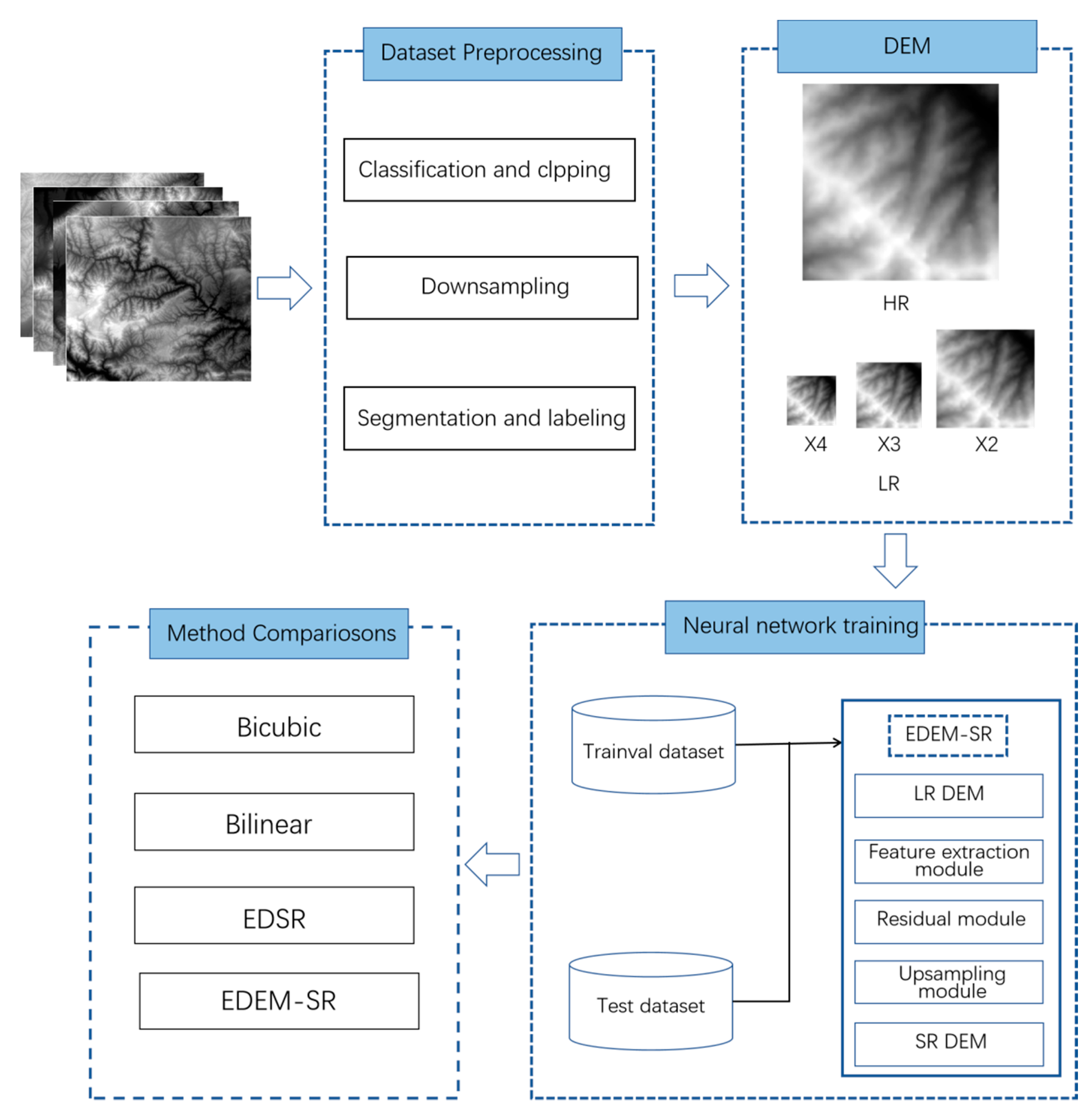
The EDEM-SR method includes: (1) data pre-processing; (2) setting up the structure of the EDEM-SR network; (3) model training; and (4) super-resolution DEM generation and evaluation. The workflow of the paper is summarized in Figure 1.

2.1. Data Pre-Processing

The corresponding data from the high- and low-resolution DEMs are used as training data, test data, and validation data. Because DEM data from different sources often have different projections, it is not easy to form the corresponding high- and low-resolution data with scales of 2, 3, and 4. In order to facilitate the experiment, the 12.5 m DEMs obtained from the PALSAR sensor of the ALOS satellite were used as the original high-resolution DEMs. We used ArcGIS to pre-process the DEMS. First, the 12.5 m DEMs was down-sampled to scales of 2, 3, and 4 by bicubic interpolation to form the corresponding low-resolution datasets. The ratio of training data, test data, and validation data was 8:1:1. Second, the original DEM data were cut out, the areas with poor data quality and urban areas were removed, and the DEM data of high quality were retained. Finally, the cropped high- and low-resolution DEM data were segmented and named systematically to form a labeled data set. In more detail, the preprocessing of the DEM data of high- and low-resolution proceeded as follows:

(1)

Bicubic down-sampling was used with the original DEM data with a resolution of 12.5 m to construct DEMs with resolutions of 25 m, 37.5 m, and 50 m.

(2)

A natural area with obvious terrain features was selected as the research area, and the high- and low-resolution DEM data were clipped to match the area in (1).

(3)

The cropped high- and low-resolution DEM data were divided into corresponding regions. For example, if the high-resolution DEM data is divided into images with 192 $\times$ 192 pixels, then the low-resolution data of scales of 2, 3, and 4 need to be divided into images with 96, 64, and 48 pixel sizes.

2.2. The Structure of the EDEM-SR Network

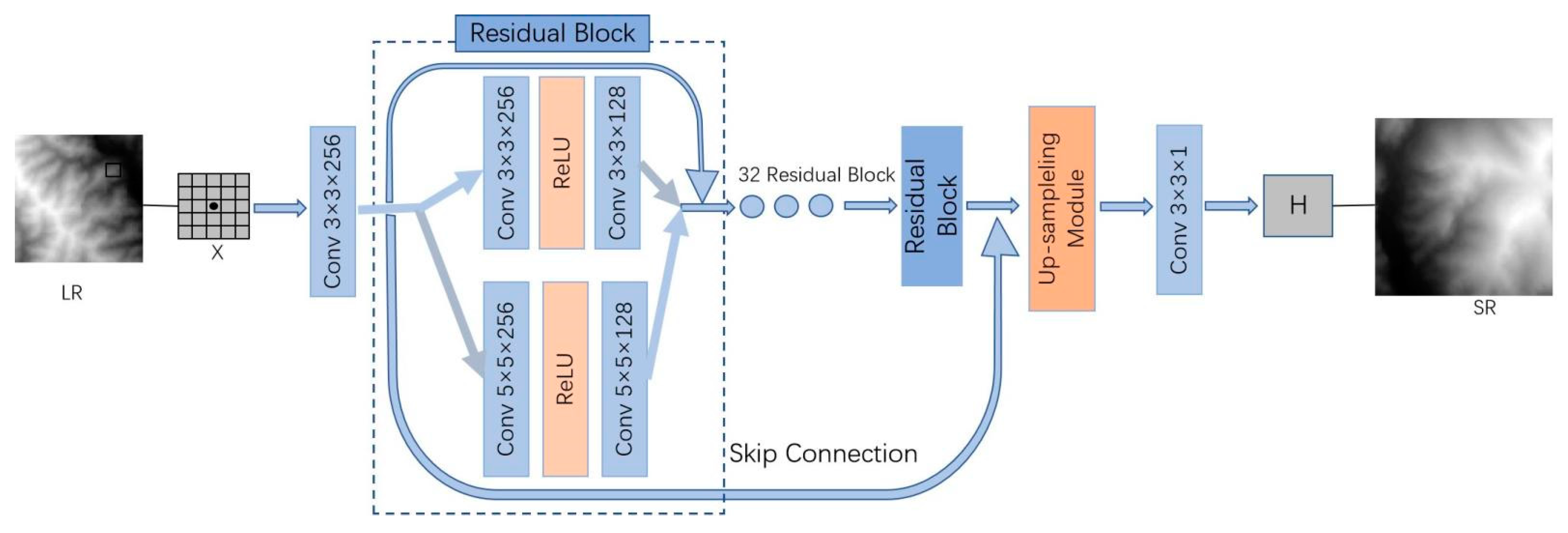
The architecture of the proposed network is shown in Figure 2 and Figure 3, and is composed of three main sub-networks, namely the feature extraction, residual, and up-sampling modules. The specific structure and functions of the three modules are as follows:

(1)

The feature extraction module consists of a convolution layer with 256 channels. Its function is to extract the features of the low-resolution DEM input data through the convolution layer, and output 256 feature maps.

(2)

The residual module consists of 32 small residual modules. The function of these residual modules is to increase the depth of the network, and further extract and fuse the feature maps generated by filters with different receptive fields. Each small residual module includes two different filter branches (i.e., 3 $\times$ 3, 5 $\times$ 5), each branch includes two convolution layers, and the activation function links the two convolution layers, as shown in Figure 3. We concatenate the feature map extracted from the two branches at the end of each residual module.

(3)

The up-sampling module consists of a sub-pixel convolution layer and a convolution layer. The function of the sub-pixel convolution module is to enlarge the size of the output image. The sub-pixel layer is used to extract $s^2$ feature maps and splice them together to enlarge the resolution of the image by s times. Then, the final super-resolution image is obtained by fusing the expected size feature images through the subsequent convolution layer. Compared with the traditional use of the deconvolution layer for up-sampling, the sub-pixel convolution layer can avoid the introduction of irrelevant information and reduce the amount of calculation.

In order to achieve better reconstruction results, the residual module of the proposed EDEM-SR has two filters with different size convolution kernels, which have different receptive fields. The size of the receptive field determines the scale of observation and affects the super-resolution. The traditional deep learning model often uses a fixed filter size, so the observation scale is limited. The multi-scale technology integration method can fuse the features extracted by different receptive field filters and better fuse the neighborhood features, which is advantageous in practice. Considering the complexity of the network, residual learning is introduced to train the network. Generally speaking, residual learning is carried out through a series of residual modules with the same structure. Different from the general convolution neural network which directly establishes the input-output mapping, the residual network calculates the difference between the desired output and input. For example, if the input is x and the target output is f(x), the goal of residual learning is to fit g(x) = f(x) − x and add the input X and G(x) to get the desired output f(x). In addition, because each layer of the convolution neural network extracts 256 feature maps, too many feature maps will lead to numerical instability in the training process. Therefore, this paper sets the residual scale to 0.1, and then multiplies the output of the convolution layer by 0.1 and adds the input x, which helps to stabilize the training process.

In summary, the EDEM-SR network can be divided into three modules. The first module extracts the feature mapping of the input DEM. The second module consists of a series of residual modules with filters of different kernel size, and further describes the extracted features as complex feature maps. These feature maps are up-sampled and high-resolution images are generated in the third and final module.

2.3. Model Training

The convolution operation can be formulated as:

$$\mathrm{a}\left(\mathrm{x}\right)=\mathsf{\sigma }\left(\mathsf{\omega }\ast \mathrm{x}+\mathrm{b}\right)$$

(1)

where $\mathsf{\sigma }(·)$ denotes the activation function, $\mathsf{\omega }$ denotes the convolution kernel for feature extraction, and b denotes the bias.

The proposed network takes the rectified linear unit (ReLU) [42] as the activation function, formulated as $\mathsf{\sigma }\left(\mathrm{x}\right)=\max \left(0,\mathrm{x}\right)$, owing to its effectiveness in nonlinear mapping. For the output X of CNN, after the activation function ReLU, the positive value remains the same, and the negative value becomes 0. ReLU has the advantages of simple calculation, fast speed and avoiding over-fitting.

In order to optimize these parameters, CNN is trained by minimizing the error between the output and the real high-resolution DEM. The error is calculated using L1 Loss as the loss function, which is defined as:

$$L1=\frac{1}{n}{\displaystyle \sum }_{i=1}^n\left(F\left(X_i-Y_i\right)\right)$$

(2)

where {$X_i$} denotes the input low-resolution DEM, $F(·)$ denotes the mapping function from low resolution to high resolution based on the CNN, {$Y_i$} denotes the input high-resolution DEM, and n denotes the number of training samples. A certain number of DEMs is taken from the training data as a batch, and a fixed size patch is randomly cropped from each picture in the batch. These patches are then concatenated together as batch data for error backpropagation. After calculating the error between the output and the actual data, the error is reduced by adaptive moment estimation using Adam [43], which is realized by updating the parameters of each layer of the neural network through the error backpropagation and iterating repeatedly. The iterative formula can be expressed as:

$$v_{W^l}={\beta }_1{v}_{W^l}+\left(1-{\beta }_1\right)\frac{\delta F}{\delta W^l},v_{W^l}^{corrected}=\frac{v_{w^l}}{1-{\beta }_1^t},$$

(3)

$$s_{W^l}={\beta }_2{s}_{W^l}+\left(1-{\beta }_2\right){(\frac{\delta F}{\delta W^l})}^2,s_{W^l}^{corrected}=\frac{s_{w^l}}{1-{\beta }_2^t},$$

(4)

$$W^l=W^l-\alpha \frac{v_{W^l}^{corrected}}{\sqrt{s_{W^l}^{corrected}}+\epsilon }$$

(5)

where t denotes the number of iterations, $v_{W^l}$ denotes the momentum, $s_{W^l}$ denotes the weighted average of differential squares, and $W^l$ denotes the filters of L-th layer.

Theoretically, the use of this transfer learning strategy based on the use of natural images to pre-train the network can make the network converge faster and reduce the amount of training sample data needed. Hence, the preliminary experiments show that the training samples used in this paper are sufficient to obtain good performance.

2.4. DEM Super-Resolution and Evaluation

According to the EDEM-SR model trained with the training dataset, the test dataset is input into the model, and the reconstructed high-resolution DEM data is output after a series of transformations. After that, the accuracy of these reconstructed high-resolution DEMs is evaluated and compared with that of other methods.

The results of the method are compared with those of the bicubic, bilinear, and EDSR methods to evaluate the super-resolution DEM performance. The bicubic and bilinear models rely on interpolation to approximate the original DEM. The EDSR model is based on convolutional neural networks, using a similar network structure to our method.

The mean absolute error (MAE), root mean squared error (RMSE), maximum elevation error ($E_{max}$), and mean error of terrain parameters ($E_{tp}$) are used to evaluate the performance of each model. In addition, all methods are tested using the test dataset.

The evaluation metrics are given by:

$$\mathrm{MAE}=\frac{1}{m}{\displaystyle \sum }_{i=1}^m\left|\left(y_i-\overline{y_i}\right)\right|$$

(6)

$$\mathrm{RMSE}=\sqrt{\frac{1}{m}{\displaystyle \sum }_{i=1}^m{\left(y_i-\overline{y_i}\right)}^2}$$

(7)

$$E_{max}=\frac{1}{m}({\displaystyle \sum }_{i=1}^m\max (\mathrm{abs}(y_i-\overline{y_i})))$$

(8)

$$E_{tp}=\frac{1}{m}{\displaystyle \sum }_{i=1}^m\left|\left(t_i-\overline{t_i}\right)\right|$$

(9)

where m denotes the number of pixels in the test samples, $y_i$ denotes the values in the original high-resolution DEM, $\overline{y_i}$ denotes the values in the reconstructed high resolution DEM, $E_{tp}$ denotes the error of the terrain parameters, $t_i$ denotes the values of the terrain parameters generated with the original high-resolution DEM, and $\overline{t_i}$ denotes the values of the terrain parameters generated with the reconstructed high resolution DEM.

3. Experiments and Results

To prove the performance of the proposed method, the results were evaluated using 800 test DEMs. The test data were not used in the neural network training, so they can well reflect the generalization ability of the network. In the experiment, the networks were implemented based on the Pytorch framework. The operating system is Ubuntu 16.04, the CPU is an Intel(R) Core(TM) i7-8700, and the GPU is a GeForce GTX 2080 equipped with 16 GB of memory. The relevant experimental configurations are listed in

Table 1. Experimental environmental configuration.

Environment	Version
Operating System	Ubuntu 16.04 (64-bit)
GPU	Nvidia GTX 2080 (8G)
CPU	Inter (R) Core i7-6800K
Batch size	16
Patch size	96
Number of ResBlock	32
Optimizer	Adam

.

In the experiment, DEM with resolutions of 25 m, 37.5 m, and 50 m were used to reconstruct a 12.5 m high-resolution DEM to evaluate the performance of the proposed model. It should be pointed out that due to the lack of real data sets of 2, 3, and 4 scales, we generated these three data sets by down-sampling the 12.5 m data in the same period, so as to ensure consistency of the data evaluation benchmarks. Four sets of results were generated with the proposed method and the bicubic, bilinear, and EDSR methods.

3.1. Study Area and Data

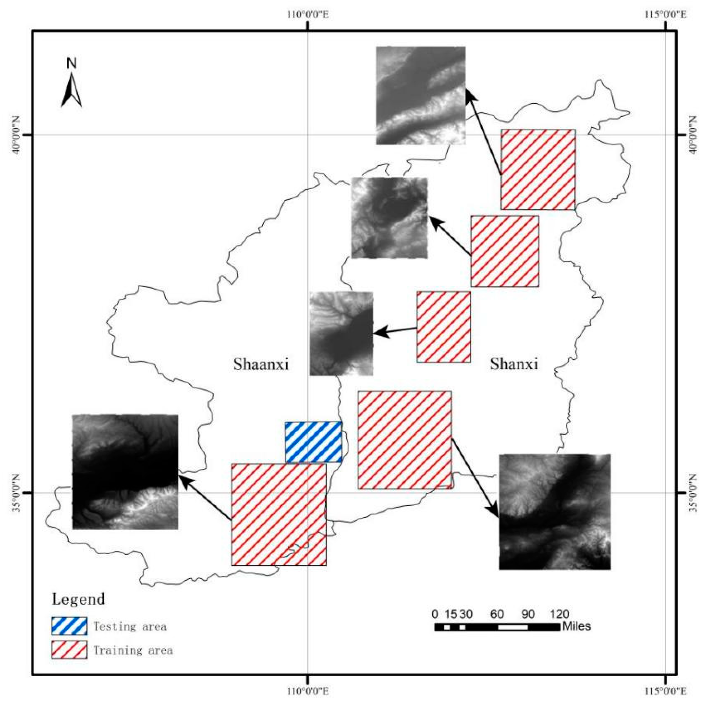
The Loess Plateau is more than 1000 km long from east to west and 750 km wide from south to north. It is located on the second step of China, with an altitude of 800–3000 m. The Loess Plateau is the largest loess area in the world. It has long been the focus of research because of its unique geomorphological features. The DEM is an important geographical data theme, however, only a small part of the region has a high-resolution DEM, which is not conducive to the analysis of a large-scale study of the Loess Plateau. A part of the Loess Plateau was selected as the study area. First, we chose the region with high-resolution DEM data on the edge of the Loess Plateau as the training data. Then, we took another area of the Loess Plateau as the test dataset and input it into the model for super-resolution DEM reconstruction. The distribution of training and test data is shown in Figure 4. The test DEM is shown in Figure 5.

The original high-resolution DEM data is divided into 192 $\times$ 192 cells. By bicubic interpolation, these high-resolution DEM are down-sampled to scales of 2, 3, and 4 times to obtain low-resolution DEM. Each sample includes a high-resolution DEM and a low-resolution DEM. We generated 8155 such samples. In this experiment, part of the Loess Plateau is used as the training set to train the model, and the trained model can be used to generate super-resolution DEMs in other regions of the Loess Plateau. For DEM reconstruction in other locations, the network can be initialized with the parameters of the existing model and then optimized with a small number of DEMs from the locations to be reconstructed to obtain good reconstruction results.

3.2. Visual Assessment

Figure 6 shows the 3D surfaces for the original DEM (Figure 6a) and the SR DEM generated with the EDEM-SR method (Figure 6b). These two images show that the DEM generated with the proposed method looks close to the original DEM and retains most of the terrain details.

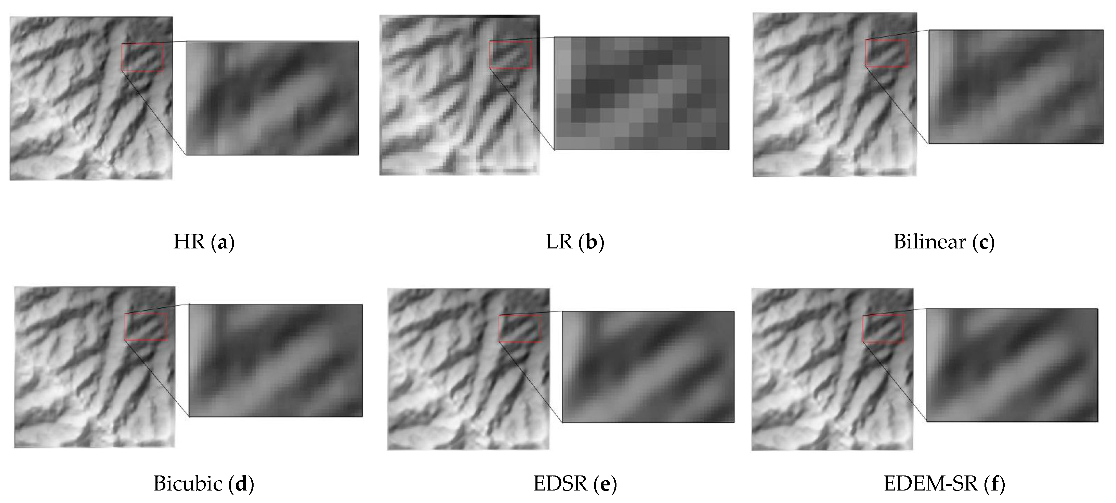
Figure 7 shows the DEM samples generalized by the different methods at a scale of 4. Naturally, with a decrease in resolution, the DEMs become rough, reflecting less terrain detail, and the difficulty of reconstruction increases. We chose the SR DEM at this scale because the differences between the four methods would be more obvious, and it is very difficult to reconstruct the 50 m low-resolution DEMs in this case. Figure 7b shows the LR DEM used to reconstruct the HR DEM. It can be seen that the LR DEM at the down-sampling scale of 4 is very rough in detail. Figure 7c shows the DEM generated with the bilinear method and the artificial texture shows the poor performance of this method for generating SR DEMs, which confirmed the previously noted disadvantage of interpolation methods losing terrain features. Figure 7d shows the DEM generated with the bicubic method that was the best performing of the two interpolation methods. It can be seen that although the DEM reconstructed by this method is close to the original DEM, it has some artificial texture. Figure 7e,f shows the DEMs generated by the two methods using CNN. The DEMs generated with this pair of methods show few visual differences and both can restore the terrain features well.

In general, bilinear has the worst reconstruction effect, with obvious artificial textures, and while the bicubic performs better and has no obvious artificial textures, the DEM reconstructed with this method has smooth terrain and poor terrain detail recovery. The methods based on deep learning provide better performance in terms of detail restoration. As expected, the high-resolution DEM reconstructed by the EDEM-SR method well reflects the valley and ridge line details.

3.3. Overall Accuracy

Table 2. Quantitative evaluation of the reconstruction effect of the test dataset.

Scale	Method	MAE (m)	RMSE (m)	${\mathbf{E}}_{\mathbf{max}}\left(\mathbf{m}\right)$
2	Bicubic	0.3048	0.6141	6.60
	Bilinear	0.5482	0.8447	7.02
	EDSR	0.2530	0.5083	4.07
	EDEM-SR	0.2520	0.5070	3.12
3	Bicubic	0.6453	1.1068	13.05
	Bilinear	0.9613	1.4563	13.37
	EDSR	0.4273	0.7414	7.69
	EDEM-SR	0.4259	0.7394	7.15
4	Bicubic	1.1824	1.7742	19.00
	Bilinear	1.7100	2.3422	19.28
	EDSR	0.8209	1.2099	12.99
	EDEM-SR	0.8012	1.1939	12.48

shows how well the DEMs reconstructed by the different methods perform with reference to the original 12.5 m ALOS high-resolution DEM data using MAE, RMSE, and $E_{max}$. These results show that the performance of different methods varies at different scales. With the increase of scales, the performance of all methods decreases, because the input low-resolution DEM contains less information. The performance of the bilinear method decreases the most, and the performance of the two deep learning methods decreases less than that of the two interpolation methods. Table 2 also shows that the proposed EDEM-SR method achieves the best results on scales of 2, 3, 4, given the lowest MAE, RMSE, and $E_{max}$ values. At the same time, the bilinear interpolation performs the worst and has the highest MAE, RMSE, and $E_{max}$ at all scales. The MAE of the proposed EDEM-SR method is about 50% lower than that of the worst bilinear method on the scale of 4. The proposed EDEM-SR model also has better results compared with the deep learning model EDSR, which has the same number of feature maps and the same number of residual modules.

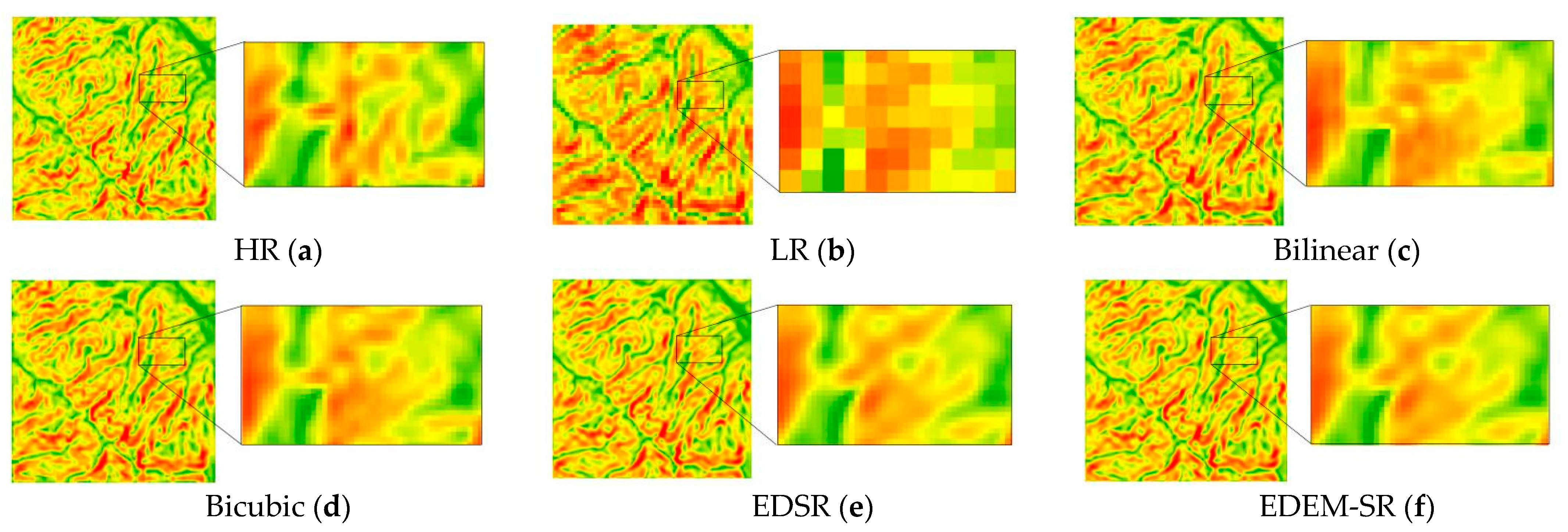
3.4. Terrain Parameters Maintenance

Figure 8 show the terrain parameters for DEMs reconstructed by different methods at the scale of 4. The color difference between Figure 8a, Figure 9a and Figure 10a and other images series shows the ability of different methods to maintain the terrain features. Figure 8c, Figure 9c and Figure 10c show the slope, aspect, and curvature for a DEM reconstructed by bilinear interpolation. From its color change, it can be seen that the bilinear method eliminates the slope decline, connects several adjacent areas with similar aspects, and the curvature is quite different from the original curvature. Specifically, the color transition of Figure 8c is not obvious, the regions separated in Figure 9a are connected in Figure 9c, and Figure 10c has an obvious artificial texture. Figure 8d, Figure 9d and Figure 10d show the terrain parameters for a sample DEM reconstructed by bicubic interpolation. The method’s performance is better than bilinear, but it has similar problems maintaining the terrain parameters. Interpolation methods all have shortcomings associated with the preservation of fuzzy and smooth terrain features. Figure 8e, Figure 9e and Figure 10e and Figure 8f, Figure 9f and Figure 10f show the results of EDSR and EDEM-SR, respectively. It can be seen that the color changes for these two methods are close to the original DEM, which confirmed that the terrain features reconstructed by the deep learning methods are close to those in the original DEM. Compared with the DEMs reconstructed by interpolation methods, the DEMs reconstructed by our method show many of the same features as the original DEM.

Table 3. Quantitative evaluation of terrain parameter retention.

Scale	Method	${\mathbf{E}}_{\mathbf{slope}}$	${\mathbf{E}}_{\mathbf{aspect}}$	${\mathbf{E}}_{\mathbf{curvature}}$
2	Bicubic	0.8450	5.8335	0.8836
	Bilinear	1.0923	6.9656	0.9659
	EDSR	0.7373	5.6483	0.7617
	EDEM-SR	0.7242	5.6194	0.7640
3	Bicubic	1.5487	10.2609	1.1521
	Bilinear	1.9537	13.3871	1.3649
	EDSR	1.0613	7.6758	0.8272
	EDEM-SR	1.0145	7.3325	0.7999
4	Bicubic	2.2151	14.8986	1.1520
	Bilinear	2.7483	17.8778	1.2238
	EDSR	1.6772	11.4672	0.8848
	EDEM-SR	1.6504	11.2404	0.8655

shows the numerical accuracy of slope, aspect, and curvature and indicates that the terrain parameters calculated by the DEM generated by the proposed EDEM-SR method have the lowest error. The errors accompanying the EDSR method are higher than for the EDEM-SR method. The numerical results in Table 3 confirm the trend evident in the maps reproduced in Figure 8. The results in Table 3 mirror those in Table 2, indicating that the performance of the interpolation methods decreases more obviously than that of the deep learning methods with an increase in scale

4. Discussion

The proposed EDEM-SR model reconstructs super-resolution DEMs at three scales. The model parameters were adjusted to improve the super-resolution performance. Through many experiments, the EDEM-SR method shows three advantages. First, compared with other interpolation methods, such as bicubic interpolation, bilinear interpolation, the DEM reconstructed by the proposed EDEM-SR method has higher accuracy, especially at large SR scales. Second, the residual module of the EDEM-SR model has two branches of filters with different convolution kernel sizes, which fully integrate the information of neighborhoods with different sizes. As a result, compared with other CNN methods, such as EDSR, the proposed EDEM-SR model shows better accuracy. Third, the EDEM-SR model shows excellent performance in preserving the details of the reconstructed DEM terrain parameters.

4.1. The Evaluation of the Precision of Using the EDEM-SR Method

Compared with the bicubic, bilinear, and EDSR methods, the proposed EDEM-SR method offered higher overall accuracy when generating SR DEMs. As shown in Table 2, the DEM reconstructed by the EDEM-SR method at the scales of 2, 3, and 4 are closer to the original high-resolution DEM with smaller MAE, RMSE, and $E_{max}$, especially in the edge region, where the interpolation method cannot obtain sufficient information and the accuracy drops significantly. In addition, with an increase of the reconstruction scale, the accuracy of the interpolation method decreases more significantly than that of the deep learning method. This is because with the increase of scale, the pixels in the low-resolution data become less, and the information obtained by the interpolation method is more limited, while deep learning methods such as EDEM-SR learn the mapping relationship between low- and high-resolution data through a large number of training samples. In super-resolution DEM reconstruction, the high-frequency information learned from other high-resolution DEM data is introduced, so these models have significant advantages in large-scale super-resolution work tasks.

Table 4. Performance of different models trained with different amounts of training data.

Scale	Method	25% Training Data (MAE)	50% Training Data (MAE)	100% Training Data (MAE)
2	EDSR	0.3713	0.2745	0.2530
	EDEM-SR	0.3745	0.2658	0.2520
3	EDSR	0.5427	0.4487	0.4273
	EDEM-SR	0.5741	0.4451	0.4259
4	EDSR	0.9044	0.8333	0.8209
	EDEM-SR	0.9399	0.8452	0.8012

shows the reconstruction effect after training the model with different sizes of training samples. It can be seen that with an increase in the number of training samples, the reconstruction effect gradually improves, and finally converges to a better result.

4.2. The Advantages of Using Double-filters

The proposed EDEM-SR method performs better than EDSR, which also is based on residual CNNs because the complete terrain structure in the real world often has different sizes. These terrain structures are represented in DEMs as sets of pixels with different extents. In order to collect complete information, a filter with an appropriate receptive field size is needed. A CNN with a single filter usually extracts information from a fixed receptive field, which cannot take every situation present in the DEM into account. Therefore, this paper proposes a residual structure with double filters, as shown in Figure 3. The information of different sized neighborhoods is collected through different size receptive fields, and then this information is fused to obtain better super-resolution performance. As shown in Table 2, the ensemble learning of the multi-filter CNN achieves the highest overall accuracy. Because multiple filters can help to obtain more important abstract features at different scales, larger filter sizes can consider more information about neighbors than smaller filter sizes and obtain the overall trend of terrain, whereas smaller filter sizes can capture the details of the object and improve the numerical accuracy. Thus, the proposed EDEM-SR model achieves better numerical accuracy compared with the EDSR method.

4.3. Retention of Terrain Parameters

From the perspective of the terrain analysis, in addition to acceptable MAE, RMSE, and $E_{max}$, maintaining terrain features is also a key measure. Figure 8, Figure 9 and Figure 10 show the terrain parameters generated by the reconstructed DEM using different methods at a scale of 4. Table 3 shows the error for mean slope ($E_{slope}$), aspect ($E_{aspect}$) and curvature ($E_{curvature}$) of different algorithms at different super-resolution scales.

From Figure 8, Figure 9 and Figure 10, one can see from the local maps that among the four methods, bilinear does the worst in maintaining terrain parameters. Bicubic is the best of the two interpolation methods and can restore details of the terrain to some extent, but it cannot restore the overall trend of the terrain very well. From the visual results, the two methods based on deep learning are better than the interpolation methods in the restoration of terrain details and the overall trend of terrain.

Table 3 quantitatively compares the performance of each method in the terrain feature preservation based on numerical accuracy, and shows how the EDEM-SR method did best in terms of maintaining the terrain parameters. All four algorithms showed good performance in the retention of terrain parameters at the scale of 2, confirmed by the small numerical errors of slope, aspect, and curvature calculated by each algorithm. But the errors in the terrain parameters obtained by the interpolation methods increased significantly at scales of 3 and 4, and the differences between the interpolation methods and the proposed EDEM-SR model became larger. The proposed EDEM-SR method offers the best performance, especially at the larger super-resolution scales.

4.4. Limitations and Future Enhancements

The proposed EDEM-SR method for super-resolution DEM reconstruction shows excellent performance. However, there are still some limitations. Although EDEM-SR achieves the lowest MAE, RMSE and $E_{max}$, at scales of 2, 3 and 4, it is not capable of training a mapping model for super-resolution at any scale. Therefore, it is necessary to consider a network architecture for full-scale super-resolution reconstruction. Although the use of double-filters can make full use of the neighborhood information, the amount of calculation increases and the computational efficiency is reduced.

In addition, the proposed model requires the training of a separate model for each type of terrain. For example, in this paper, the model trained by the proposed method has achieved good performance using mountainous terrain on the Loess Plateau. When reconstructing DEMs for other terrain types, such as flat or urbanized areas, we need to take the current model as the initial model, and use a small number of DEMs of these types to adjust model parameters to obtain the best results. Besides, for urban DEMs, LiDAR data with a resolution of around 1m is generally used, and for this type of high-resolution data, more data needs to be used to train a better model compared with reconstructing a natural area DEM with a resolution of 10 m.

Finally, the EDEM-SR method still focuses on the overall characteristics of the terrain, without considering the high-resolution terrain feature points in local areas. The method may offer better results if the reconstruction results of the super-resolution model were constrained by local terrain features.

Future work will focus on training terrain features into the network to constrain the super-resolution results, so that the SR DEM can retain more terrain features. We also plan to use higher resolution DEMs and open-access low-resolution DEMs to generate training data, instead of just down-sampling high-resolution DEMs to obtain training data.

5. Conclusions

In this paper, an EDEM-SR method with double filters was proposed for super-resolution DEM reconstruction. Based on the data fusion between different neighborhoods of low-resolution DEMs, this method can reconstruct a high-resolution DEM with better numerical accuracy and preservation of the original DEM terrain features. Comparing the accuracy of the high-resolution DEMs reconstructed by different methods, the EDEM-SR model achieves the best performance at scales of 2, 3, and 4. The experimental results show that, with the same residual module and the same number of feature maps, the reconstruction accuracy is improved by fusing the feature maps of filters with different convolution kernel sizes.

The results show that using the EDEM-SR method to build a mapping model from high- and low-resolution data of a certain region offers a promising solution for generating SR DEMs. The high-resolution DEMs of other regions can be reconstructed using the mapping model with low-resolution DEMs. In future work, local terrain features should be considered to constrain the results of super-resolution DEM reconstruction.